Weighted Gradient Feature Extraction Based on Multiscale Sub-Blocks for 3D Facial Recognition in Bimodal Images

School of Computer Science and Engineering, Hebei University of Technology, Tianjin 300400, China
*
Authors to whom correspondence should be addressed.
Information 2018, 9(3), 48; https://doi.org/10.3390/info9030048
Submission received: 6 January 2018
/
Revised: 3 February 2018
/
Accepted: 19 February 2018
/
Published: 28 February 2018
Abstract
:In this paper, we propose a bimodal 3D facial recognition method aimed at increasing the recognition rate and reducing the effect of illumination, pose, expression, ages, and occlusion on facial recognition. There are two features extracted from the multiscale sub-blocks in both the 3D mode depth map and 2D mode intensity map, which are the local gradient pattern (LGP) feature and the weighted histogram of gradient orientation (WHGO) feature. LGP and WHGO features are cascaded to form the 3D facial feature vector LGP-WHGO, and are further trained and identified by the support vector machine (SVM). Experiments on the CASIA database, FRGC v2.0 database, and Bosphorus database show that, the proposed method can efficiently extract the structure information and texture information of the facial image, and have a robustness to illumination, expression, occlusion and pose.
1. Introduction
With the rapid development of technology and societal progress, efficient authentication is needed in many fields, e.g., surveillance, human–computer interaction, and biometric identification. The face, as a unique personal identity, has many advantages: it allows for good interaction and is stable, difficult to counterfeit, and cannot be lost, etc., has been widely used in authentication. In recent years, the improvement of 3D data acquisition on devices and computer processing capabilities make a rapid development of the 3D facial recognition technology. Compared with a 2D face, which is easily affected by external factors, such as facial expression, pose, illumination, and age variations, 3D data can express facial information more comprehensively and richly, and better reflect the geometric structure of the human face. Even though there is some loss of information caused by external conditions, it is still much smaller than with 2D data, so more and more researchers are focusing on the 3D field.
The existing 3D facial recognition techniques can be roughly classified into three categories: globally based, locally based, and multimodal hybrid methods. Global feature-based methods often extract statistical features from depth images [1]. Thakare et al. [2] used the principal component analysis (PCA) components of the normalized depth image and moment invariants on mesh images to implement an automatic 3D facial recognition system based on the fuzzy neural network (FNN). Independent component analysis (ICA) [3], linear discriminant analysis (LDA) [4], and sparse preserving projection (SPP) [5] are also used to extract global facial features. The global features mainly describe the properties of the whole face, and have rotation invariance, simple calculation, and intuitive representation; however, they have high dimensional features, and cannot describe detailed changes of the face.
The local feature-based methods use stable local invariance features, such as facial curves, local descriptors, and curvature to match and identify faces, which can be applied to both the depth image and the 3D model. Li et al. [6] extended the scale invariant feature transformation (SIFT)-like matching framework to mesh data, and used two curvature-based key point detectors to repeat the complementary position in the facial scan with high local curvature [7]. Guo et al. [8] represented the 3D face by a set of key points, and then used the relevant rotational projection statistics (RoPS) descriptor to expression variations. Lei et al. [9] proposed a set of local key point-based multiple triangle statistics (KMTS), which is useful for partial facial data, large facial expressions, and pose variations. Tang et al. [10] presented a 3D face method by using keypoint detection, description, and a matching framework based on three principle curvature measures. Yu et al. [11] used the ridge and valley curve of the face to represent and match 3D surfaces, which are called 3D directional vertices (3D2V); using sparsely-distributed structure vertices, the structural information is transferred from its deleted neighboring points. Hariri et al. [12] used geodesic distances on the manifold as the covariance metrics for 3D face matching and recognition. Emambakhsh et al. [13] proposed a feature extraction algorithm, which is based on the normal surfaces of Gabor-wavelet-filtered depth images. With this method, a set of spherical patches and curves are positioned over the nasal region to provide the feature descriptors. Okuwobi et al. [14] used the principal curvature direction and the normal surface vector to obtain directional discrimination, in order to improve the recognition performance. The local feature-based methods are robust for image transformations such as illumination, rotation, and viewpoint changes, and their feature descriptors have low dimensions and are easy to match quickly. However, the local features mainly describe the changes in details of the human face, and are inferior to the global features in describing the facial contour features.
The bimodal hybrid methods refer to the combination of 2D and 3D modes. The most common method is to combine the intensity map (2D mode) with the depth map (3D mode) for facial recognition. The depth map is equivalent to a projection of three-dimensional information in a two-dimensional plane, and contains the information of the face’s structure. The intensity map contains the texture information of the face, and the features extracted from these two kinds of images can be more complete and richer for representing the identity information of the face. The recognition rate is higher than in a single kind of image feature extraction. Kakadiaris et al. [15] used a combination of 3D and 2D data for face alignment and the normalization of pose and illumination, and then constructed 3D deformable model with these data. This framework is more practical than 3D–3D and more accurate than 2D–2D. However, the recognition rate relies on the facial fitting in 2D mode. Elaiwat et al. [16] proposed a fully automated, multimodal Curvelet-based approach, which uses a multimodal detector to repeatedly identify key points on textural and geometric local face surfaces. Zhang et al. [17] proposed a cross-modal deep learning method, in which 2D and 2.5D facial features were extracted by two convolutional neural networks (CNN), both individually and fused on the matched face features. Ouamane et al. [18] extracted multiple features, including multi-scale local binary patterns (MSLBP), statistical local features (SLF), Gabor wavelets, and scale invariant feature transformation (SIFT), and used combinations of these different features for 3D and 2D multimodal score-level fusion to get the best result. However, there are different kinds of feature combinations, so there is no guarantee that a given feature combination can achieve the best effect on different databases. Subsequently, Ouamane et al. [19] proposed a high-order tensor encoded by 2D and 3D face images, and used different tensor representation as the basis for multimodal data fusion. This method needed to consider a large number of feature combinations and subspace combinations, which increased the time complexity. To overcome the uncontrolled environments in 3D facial recognition, Torkhani et al. [20] used 3D-to-2D face mesh deformation to obtain the 2D mode, and then extracted facial features by combining edge maps with an extended Gabor curvature in the 2D projected face meshes. Bobulski [21] presented the full ergodic two-dimensional Hide Markov model (2DHMM), which overcomes the drawback of information lost during the conversion to a one-dimensional features vector.
In addition, there are some 3D facial recognition methods based on the direct matching of airspace, without extracting features [22]. The 3D point cloud data was used as the processing object, and the similarity calculation between input face and reference face models was performed directly, based on the iterative closest point (ICP). Some other methods, i.e., convolutional neural networks, are commonly used to process human face images for recognition [23,24,25].
To extract facial information comprehensively and avoid a complex process of 3D point cloud data, this paper proposes a bimodal 3D facial recognition method, which can reduce the time cost and space complexity, as well as improving recognition efficiency. There are two kind of features extracted from the multiscale sub-block’s 3D mode depth map and 2D mode intensity map, which are the local gradient pattern (LGP) feature and the weighted histogram of gradient orientation (WHGO) feature [26]. The gradient is robust for illumination transformation, and reflects the local region information contained in the image; thus, by calculating the gradient edge response, relative gradients, and the occurrence frequency of those gradients in different directions, these two features efficiently express the human face. The proposed multimodal fusion method reduces complexity and improves recognition speed and efficiency.
The contributions of this paper:
- Describe a method which can automatically recognize human faces by using depth and intensity maps converted from 3D point cloud data, which are used to provide structural and texture information.
- Extract features from multiscale sub-blocks’ bimodal maps for mining essential facial features.
- Propose the feature of the local gradient pattern (LGP), and combine LGP with the weighted histogram of gradient orientation (WHGO) to constitute the LGP-WHGO descriptor for extracting the texture and structural features.
The remainder of the paper is organized as follows. In Section 2, the whole theoretical method of 3D face recognition is given in detail, and the pre-process of 3D facial data is introduced. Section 3 introduces the specific process of weighted multiscale sub-blocks. In Section 3, the experiments and analysis are presented. Conclusions and future developments end the paper.
2. Weighted Gradient Feature Extraction Based on Multi-Scale Sub-Blocks for 3D Facial Recognition in Bimodal Images
The proposed framework consists of five main phases, including preprocessing, operation of weighted multiscale sub-blocks (on both the depth and intensity map), feature extraction, dimension reduction, and the validation process. In each stage, several algorithms are applied, and the result of each stage is the input for the next stage. The complete process is depicted in Procedure 1.
| Procedure 1: The complete process of 3D facial recognition. |
| Data: 3D point cloud data |
Result: Recognition rate
|
2.1. Three-Dimensional Facial Pre-Processing
The amount of face point cloud data acquired by 3D laser scanner is usually huge. Besides facial data, it also contains the hair, neck, shoulders, and other useless information, even interference factors such as holes, spikes, and different postures, which bring significant challenges for 3D facial recognition. Therefore, it is necessary to transform the 3D facial point cloud data to the depth and intensity images, which only contain the facial features. Depth maps contain facial structure features, which are characterized by high computational speed and classification accuracy, but these features can only describe the general structure of different faces, and cannot overcome the subtle textural changes of the same face. Therefore, the recognition rate is not very accurate when distinguishing similar categories. The intensity maps contain precisely the characteristics of the human facial texture. In this paper, the depth map and the intensity map are combined and complemented, in order to improve the recognition performance.
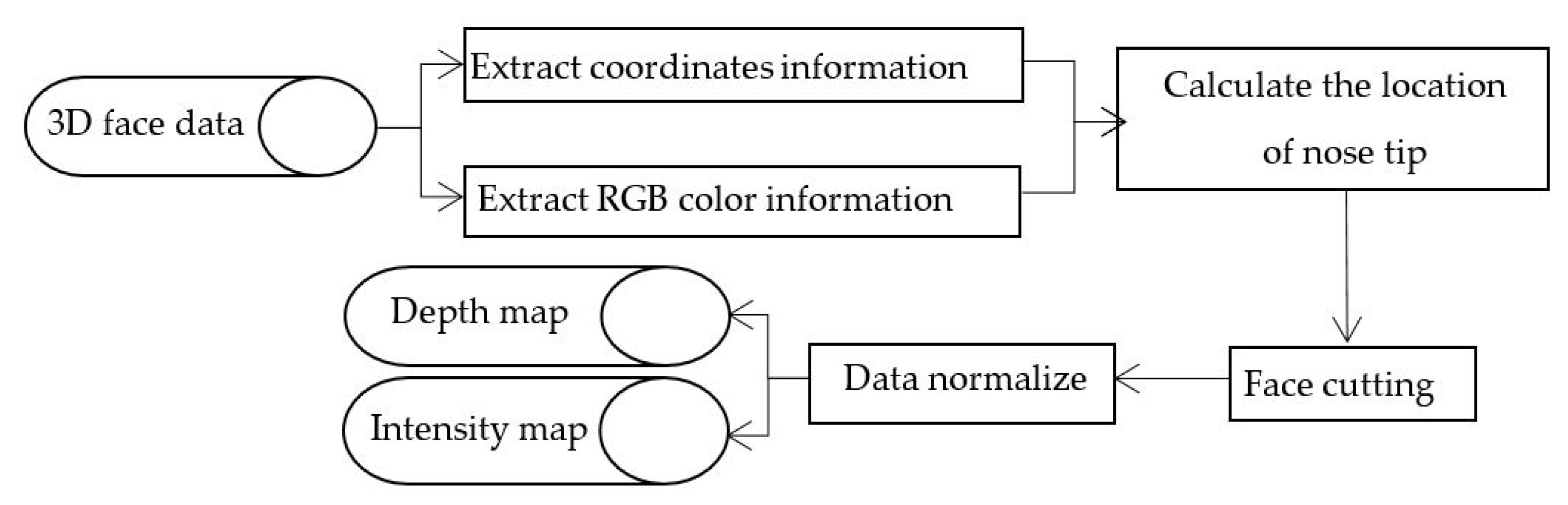
Face point cloud data contains the spatial geometry information and color texture information, which is useful to get the depth and intensity maps. There are four steps to transform face point cloud data into a depth map. First, extract the geometric coordinate information and RGB color information of the 3D sampling point. Second, calculate the position of the nose tip, which is the highest point in the central face axis with constant rigid characteristics. Third, use the nose tip as the center of the sphere for face cutting, which removes the hair, shoulders, neck and other redundant information, and only retains the area of the face. Finally, the obtained geometry data and color texture data are normalized, including smoothing, de-noising, hole filling, attitude correction, histogram equalization, and other operations. The normalized data is projected onto the two-dimensional planar grid, and the average of the z coordinates of the point cloud in the grid is calculated as the pixel value of the depth map.
Similarly, the intensity image is obtained by converting the RGB color information of each face point cloud in the facial region into intensity value information.
2.2. Weighted Multiscale Sub-Block Partitions
To mine more essential features of images, multiscale sub-block partition is performed before extracting facial structural and texture features. The multiscale approach is inspired by the construction of the Gaussian scale space in the SIFT [6]. The scale space of an image is denoted as the function , which is produced from the convolution of a variable-scale Gaussian function , with an input image of :
where “*” is the convolution operation, and
The larger the value of , the lower the resolution of the image and the rougher the scale; conversely, the finer the detail the image contains. In this paper, only three scales in the Gaussian space are considered. Otherwise, the excessive number of pictures will affect the experimental results. Gaussian scale space is assigned different weights, while weighted multiscale space is defined as:
where is weight matrix of the multiscale space, the coefficient controls the magnitude of , and the coefficient controls the size of the image in different octaves, which means that size of the first octave of the image is times that of the rth octave. The result of the weighted multiscale operation is shown in Figure 3; these nine images are generated after the operation, so there are three octaves produced, each with three images. In this paper, = 21/3, = 1.6 (refer to Lowe’s literature [6]), = 0.5, = 0.3, and = 0.2.
Sub-block partitioning means segmenting the image into sub-blocks based on the multiscale, then the features of each sub-block are extracted in a certain sequence, and all of the sub-block features of the entire image are cascaded together. The size of sub-blocks also affects the recognition accuracy. If the sub-block is too large, the details cannot be well represented. Conversely, the characteristics of important parts, such as eyes, nose, and mouth will be ignored. In this paper, sub-blocks are weighted and cascaded as follows:
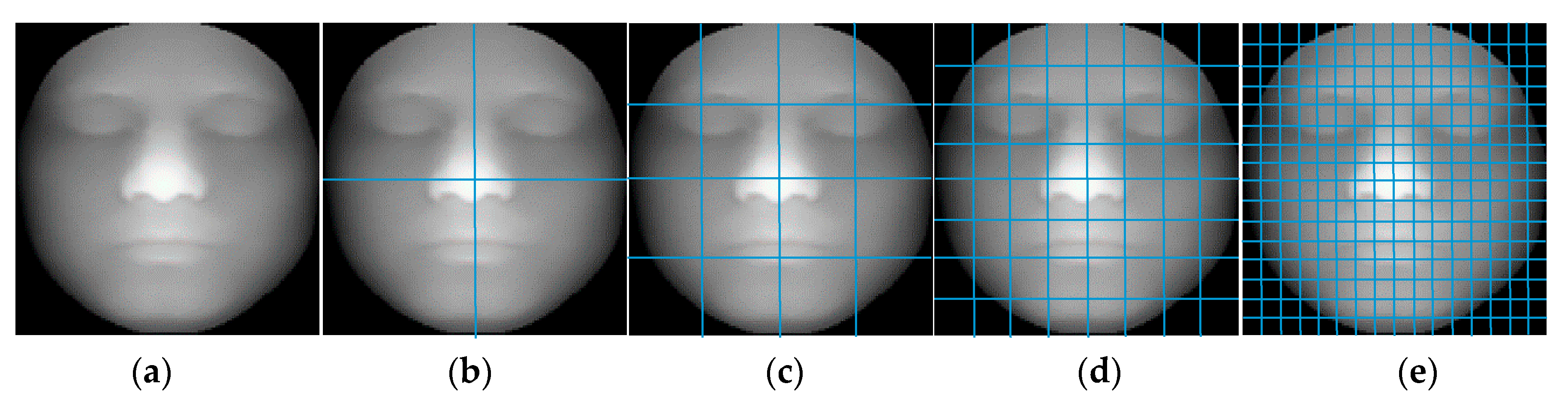
where is the sub-blocks’ function, and the input image is divided into sub-blocks, while is weight coefficient. In this paper, b1 = 0.1, b2 = 0.2, b3 = 0.3, and b4 = 0.4. The sub-blocks’ operation is shown in Figure 4.
2.3. Local Gradient Pattern and Weighted Histogram of Gradient Orientation
Based on the benefits of the gradient feature and inspired by Zhou [26], the method of weighted gradient feature extraction in the bimodal image for 3D facial recognition is proposed in this paper. This method uses two descriptors, local gradient pattern (LGP) and weighted histogram of gradient orientation (WHGO), and cascades them to be LGP-WHGO, which can extract both the structural and the texture features of face images.
The LGP descriptor is improved by local directional pattern (LDP) [27] and gradient binary pattern (GBP) [26]. LGP not only uses the advantages of two descriptors, but also overcomes the disadvantage that LDP does not take negative values into account, and the number of gradient directions of GBP is not rich enough. The relative gradients are made full use of with LGP to express the characteristics of each pixel, so that the gradient value is more stable than the intensity value. LGP takes edge response values and relative gradients going in different directions into account; thus, the extracted features from the LGP descriptor are more abundant, and the LGP descriptor is robust to non-monotonic lighting and randomly generated noise.
2.3.1. Local Directional Pattern
The local directional pattern [27] of each pixel is an eight-bit binary code calculated by comparing the edge response values (m0, …, m7) of different directions in a 3 × 3 neighborhood. The edge response values are obtained by convolving the 3 × 3 neighborhood with eight Kirsch masks. Kirsch masks M0 to M7 are shown in Figure 5. Then, the top k response values |mi| (i = 0, …, 7) are selected, and the corresponding directional bits are set to 1. The remaining (8 − k) bits are set to 0, and the binary expression of a local directional pattern is as follows:
where is the k-th largest response value.
2.3.2. Gradient Binary Pattern
The GBP [26] was inspired by the local binary pattern (LBP) [28]. Unlike the LBP operator, which describes each pixel by the relative intensity values of its neighboring pixels, the GBP operator describes each pixel by the relative gradient on different directions of the pixel. Two simple one-dimensional masks [−1 0 1] and [−1 0 1]T were adopted to convolute with the 3 × 3 neighborhood, centered with pixel , and the gradients were calculated in the horizontal and vertical directions, respectively, i.e., and . Gradients on the diagonal directions (i.e., and ) are calculated by two two-dimensional masks [0 0 1; 0 0 0; −1 0 0] and [−1 0 0; 0 0 0; 0 0 1], which is also convoluted with a 3 × 3 neighborhood centered with pixel . The relative gradient in four different directions is shown in Figure 6a. The GBP value of the pixel can be calculated as follows:
2.3.3. Local Gradient Pattern
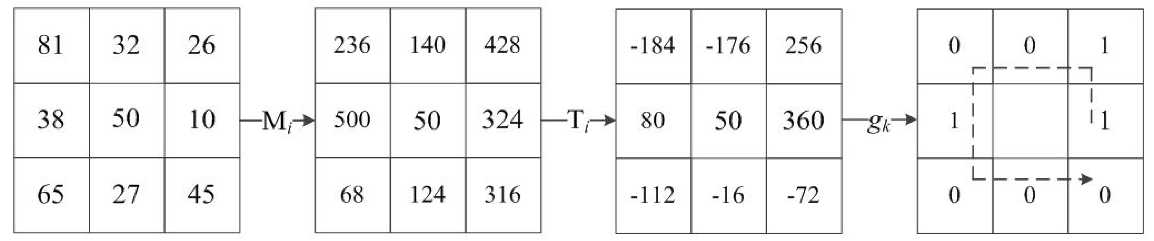
The LGP combines LDP [27] and GBP [26]. To calculate the LGP operator, firstly, the eight edge response values m0 to m7 are calculated by convolving the 3 × 3 neighborhood of each pixel with Kirsch masks; then, the relative gradients of each pixel in eight directions are calculated by the edge response values and eight direction masks.
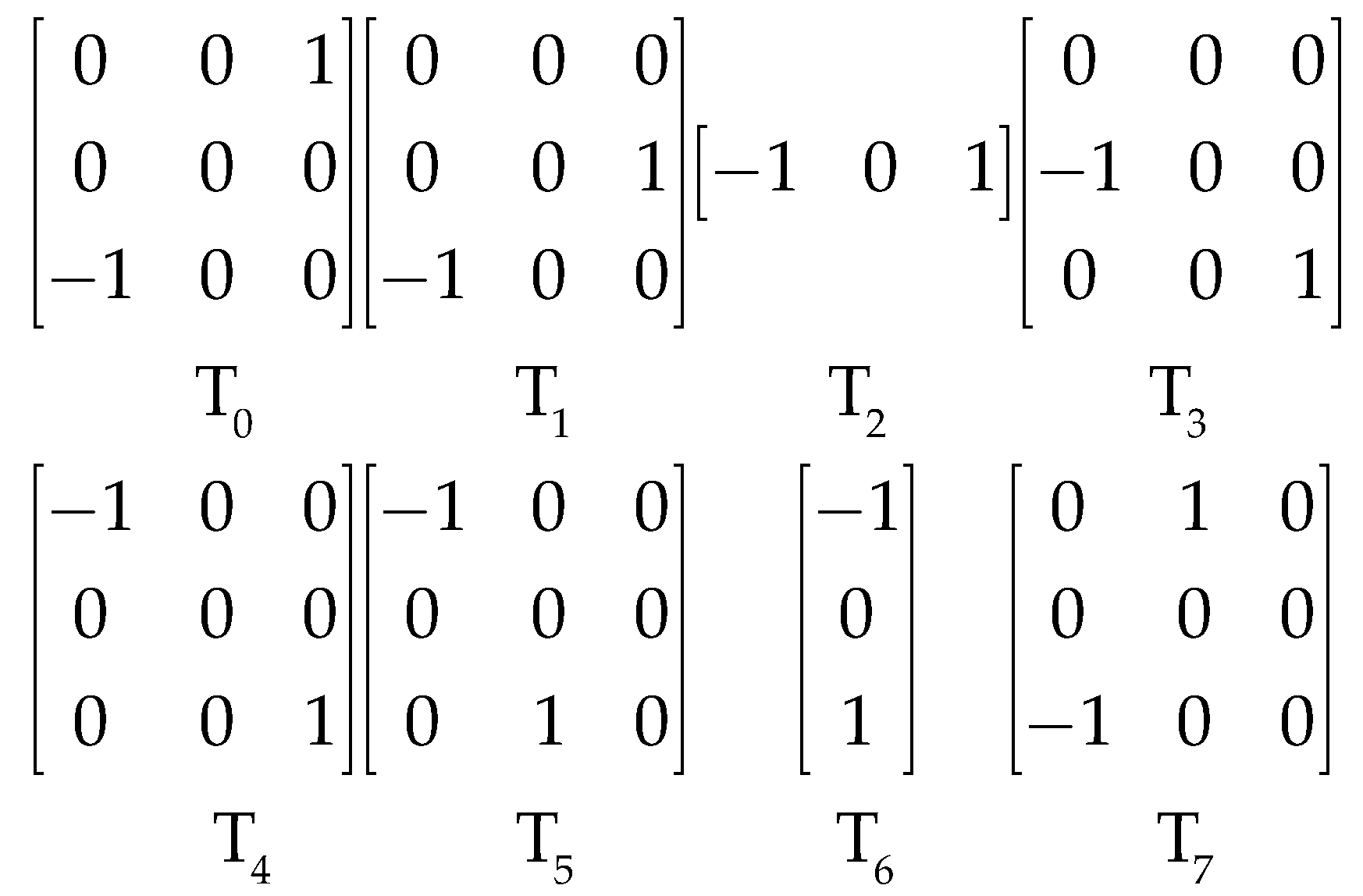
To calculate the relative gradients of each pixel in eight directions, four non-diagonal directions need to be added to enrich the four directions (D1, D2, D3, D4) used the GBP descriptor. We adopted four two-dimensional masks [0 0 0; 0 0 1; −1 0 0], [0 0 0; −1 0 0; 0 0 1], [−1 0 0; 0 0 0; 0 1 0] and [0 1 0; 0 0 0; −1 0 0] to calculate the four additional directions, i.e., D1′, D2′, D3′, and D4′, as shown in Figure 6b. Eight directional masks, T0 to T7, are shown in Figure 7.
The corresponding relationships between the direction and the magnitude of the relative gradients of the edge response value and the calculation process can also be expressed as follows:
Then the top k values are selected, and the corresponding directional bits are set to 1, the remaining bits are set to 0. The LGP value of a pixel at the position can be calculated as follows:
where is the kth value in ; in this paper, k = 3. The complete process is shown in Figure 8. An example of LGP code at k = 3 is shown in Figure 9.
2.4. Weighted Histogram of Gradient Orientation
The WHGO [26] descriptor uses the gradient magnitude as the weight of the histogram of gradient orientation. The detailed description and the calculation of the descriptor are as follows.
The original gradient orientations are spaced over; the gradient orientation is quantized into discrete orientation bins using the following equation:
where is the orientation bin for pixel , and is the corresponding gradient orientation for the pixel , B is the number of orientation bins, and the function ceil(m) is a top integral function.
Once this calculation is complete, the value of the pixel in the image is replaced by the value of its discrete orientation bin . Furthermore, to increase the spatial attributes, more image details are stored to deal with the rotation displacement of facial images, as with the sub-block operation illustrated in Section 2.2. There are also four types of block methods used here, which are 2 × 2, 4 × 4, 8 × 8, and 16 × 16—therefore, . In each sub-block, the pixel gradient magnitude is used to as its weight of orientation, and the weight of the sub-block is defined as
where indicates which sub-block the pixel belongs to, is the k-th dimension of the histogram, and is the gradient magnitude of the pixel . The final WHGO descriptor is calculated as
where is the number of pixels of the sub-block .
2.5. Dimension Reduction Processing
The LGP-WHGO is obtained by cascading the LGP and WHGO features extracted from both the depth map and the intensity map, but there is a redundant feature dimension that needs to be removed, due to the facial cutting or the high-similarity features among all of the faces in the databases. This paper defines a similarity threshold to remove the redundant features. The similarity of jth dimension feature is defined as
where N is the number of database samples, the matrix A represents the feature matrix extracted by the entire sample dataset, Ai is the feature vector of the ith sample, and is the sample mean of all feature vectors.
The final LGP-WHGO feature vector to represent face identity is obtained after dimension reduction processing.
3. Experiments and Results
The experimental environment was a PC, with Inter(R) Core(TM) i5-3210M CPU 2.50 GHz, 4GB RAM, and a Microsoft Windows 7 operating system; the programming platform was MATLAB R2014a. To verify the proposed method, experiments were carried on three public 3D datasets: CASIA, FRGC v2.0, and Bosphorus.
The CASIA database contains 123 subjects, each subject having 37 or 38 images with individual variations of poses, expression, illumination, combined changes in expression under illumination, and poses as expressions. The FRGC v2.0 dataset consists of 4950 3D scans (557 subjects) along with their texture images (2D), in the presence of significant variations in facial expressions, illumination conditions, age, hairstyle, and limited pose variations. The Bosphorus database consists of 4666 3D scans (105 subjects), and each face scan has four files (coordinate file, color image file, 2D landmark file, and 3D landmark file) with neutral poses and expressions, lower face action units, upper face action units, action unit combinations, emotional expressions, yaw rotations, pitch rotations, cross rotations, and occlusions. These three databases are the most widely used in the field of facial recognition.
This paper uses the k-fold cross-validation. The selected dataset is equally divided into nine sub-datasets. The data of each sub-dataset is randomly but uniformly selected. One sub-dataset is used as the testing set, and the remaining are used as training sets, and each experiment will obtain the corresponding recognition rate, which is the average recognition rate of k experiments as a k-fold cross-validation rate of recognition. According to the number of images involved in the training sets and the testing set, the experiments on the CASIA and FRGC v2.0 databases used a nine-fold cross-validation, and the experiments on Bosphorus database used a 10-fold cross-validation.
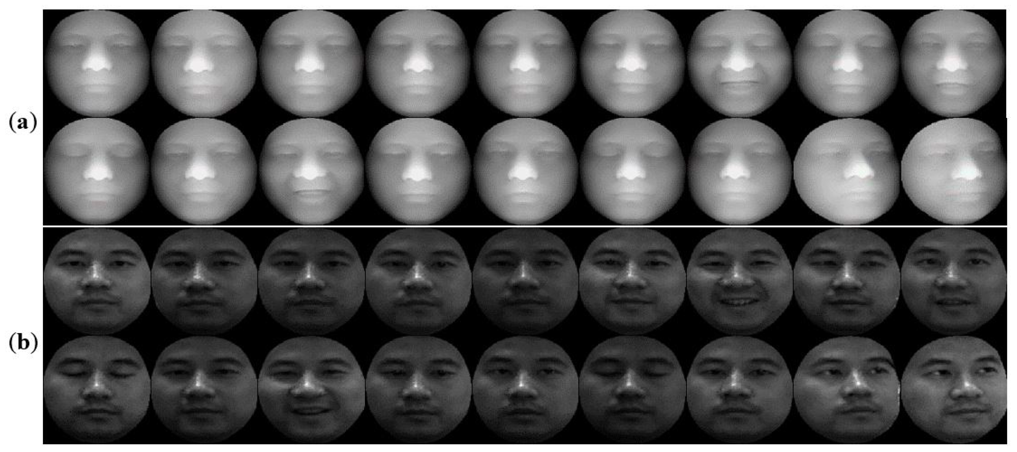
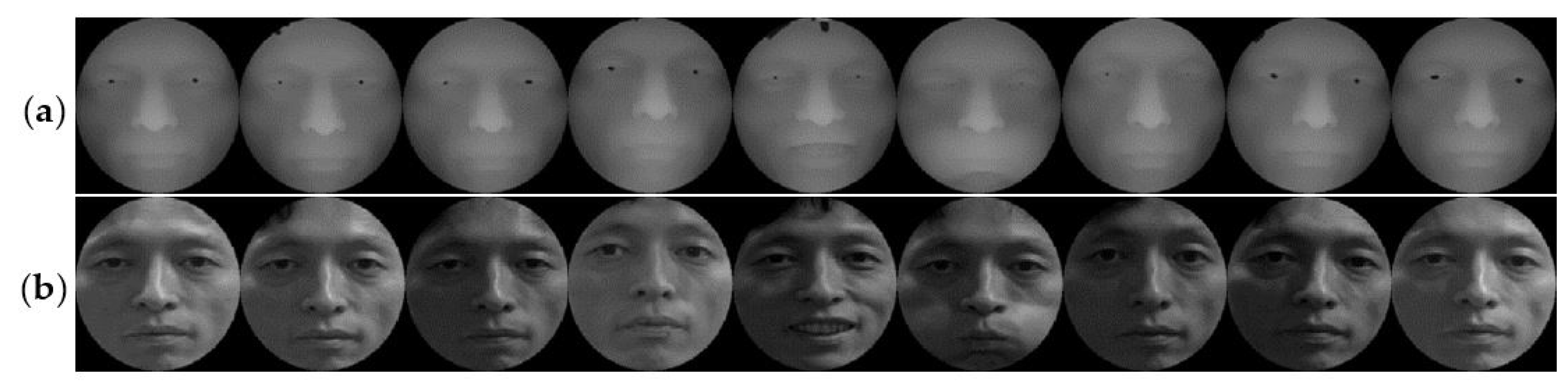
Each database has been experimenting with two groups of images. For the CASIA database, the first group includes 40 people selected, with 36 pictures randomly selected for each person. An example is shown in Figure 10. In Figure 10a,b, there are 18 samples of the depth and intensity maps, respectively, and these samples involve illumination, expressions, and pose variations. The second group is based on the previous increase of 40 people’s data. For the FRGC v2.0 database, the first group selected 80 people (18 pictures per person) in the database randomly, and an example is shown in Figure 11. In Figure 11a,b there are nine samples of the depth and intensity maps, respectively, and these samples involve illumination, expressions, and age variations. The second group is based on the previous increase of 80 people’s data. For the Bosphorus database, the first group includes 40 people selected, with 80 pictures per person, and an example is shown in Figure 12. In Figure 12a,b, there are 40 samples of the depth and intensity maps, and these samples involve expressions, occlusion (eye occlusion, mouth occlusion, eyeglasses occlusion, and hair occlusion), and pose variations (yaw 10, 20, 30, 45 degrees). The second group is based on the previous increase of 40 people’s data.
3.1. Experiments with Different Descriptors on Recognition Rate
In this section, the five descriptors, including LGP, WHGO [26], LBP [28], LDP [27], and GBP [26] are extracted from both the depth map (DM) and intensity map (IM), and the obtained maps are shown in Figure 13. The feature histograms are shown in Figure 14. The LGP maps in Figure 13e and the WHGO images in Figure 13f show that both descriptors retain facial structural and texture properties effectively, but LGP maps represent the features of the human face better than LBP, LDP, and GBP descriptors.
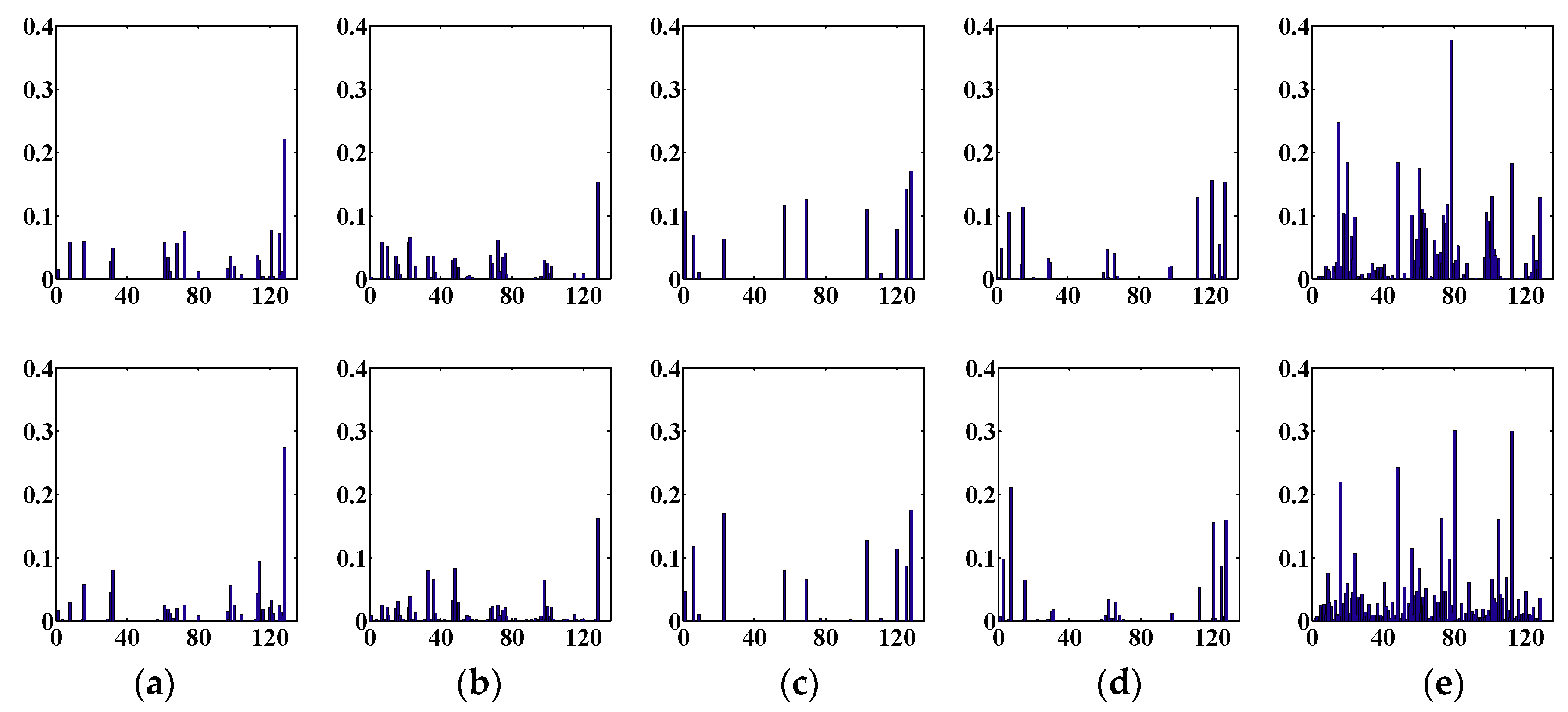
Figure 14 shows feature histograms of the five descriptors. The first line is the five different feature histograms of the depth map, and the second line shows the five different feature histograms of the intensity map. The abscissa of each feature histogram is the gradient orientation after being quantized, and the ordinate is the weighted frequency value. As can be seen from Figure 14, the trend of the distribution of the histograms for each column of features is roughly the same, but there are subtle differences because the depth and intensity maps contain different information, even when they are converted from the same face image. From each row of the five histograms on view, the LBP and LDP histogram distributions are the most uniform. There are fewer features in the GBP feature histogram distribution. The performance of LGP is better than GBP, and the peak and valley values are visible, so the feature histogram distribution is more abundant. Although the histogram of GBP has noticeable peaks and valleys, the characteristics are scarce, and the peak–valley distribution by LGP is more visibly abundant. The results of the WHGO descriptor are very good. The performance of each descriptor needs to be displayed in combination with the recognition rate of each group of experiments.
The recognition rate (RR) comparisons of the LGP, WHGO [26], LBP [28], LDP [27], and GBP [26] descriptors are presented in the CASIA database, the FRGC v2.0 database, and the Bosphorus database, respectively shown in Table 1, Table 2 and Table 3. All five descriptors are extracted from the depth map (DM), then concatenate descriptors of the corresponding intensity map (IM); finally, after the dimension reduction and removal of the redundant information, the final feature is taken as the general characteristics of the identity, and used for identification. In the tables below, STr is the size of the training set, and STe is the size of the testing set.
3.2. Experiments with Different Combination of Descriptors
3.3. Comparison with State-of-the-Art Methods
The proposed LGP-WHGO method was compared with the state-of-art facial recognition methods in two databases. The method in [2] is the global feature-based method, the method in [13] is the local feature-based method, and the methods in [15,16,17,18,19] are multimodal hybrid methods. Table 7 and Table 8 are RR comparisons with state-of-art methods on the CASIA and FRGC v2.0 databases, respectively.
As can be seen from Table 7, Table 8 and Table 9, compared with facial recognition methods in recent years, the RR of this paper is quite encouraging. When the CASIA experimental dataset contained facial images which deflected 20–30 degrees, the RR rises to 98.61%. For the FRGC database, the RR of the proposed method reaches 98.06% when involving illumination, expressions, and age variations. The Bosphorus experimental dataset contains not only yaw rotation face images (yaw 10, 20, 30, and 45 degrees), but also occlusion face images (eye, mouth, eyeglasses, hair occlusion)—with that dataset, the RR reached 96.75%.
Methods in [2,17] used the trained advantages of neural networks to extract features and classification. The method in [18] used different combinations of features, including MSLBP, SLF, Gabor wavelets, and SIFT for classification. The method in [19] not only directly used the point cloud data for calculation, but also used multiple features and subspace combinations, especially in the Bosphorus database experiments. The training and testing sets contained only neutral face and basic expressions, and did not consider occlusion faces. The method in [16] directly used 3D models for detecting key points, and the Bosphorus database experiments did not contain occlusion faces. The method in [17] used three 3D databases (BU3D, Bosphorus, and CASIA) to train the model, and the authors’ experiments demonstrate the method’s interesting performance. Regarding time cost, the disadvantage of these methods is that they are complicated and time-consuming. The method of this paper uses structural features of the depth map and texture features of the intensity map extracted by the LGP-WHGO descriptor for recognition. As a result, this method saves time and has a high practicality compared with other algorithms, primarily through use the 3D point cloud data for calculation directly.
4. Discussion
We have presented a 3D facial recognition method. To reduce the effect of illumination, pose, expression, ages, and occlusion on facial recognition, our method transforms 3D point cloud data to depth and intensity maps. The depth map contains face structure features, and the intensity map contains the characteristics of the human face texture. On multiscale sub-blocks, the proposed LGP-WHGO, combined with the LGP and WHGO descriptors, can capture more structural features and texture features, and improve the recognition performance. Experimental results show that the recognition rates of LGP-WHGO are higher than that using single image information. Using the CASIA database with non-frontal pose images deflected 20–30 degrees, the recognition rate reached 98.61%, which is a very significant result. In the FRGC v2.0 database experiments, the highest recognition rate also reached 98.06%. With the Bosphorus database, the experimental dataset contains not only yaw rotation of face images (yaw 10, 20, 30, and 45 degrees), but also occlusion variations of face images (eye, mouth, eyeglasses, hair occlusion), still the RR comes up to 96.75%.
In this paper, the proposed algorithm is meant mainly to identify faces that have a small area of the face occlusion or poses between 10 and 45 degrees of deflection. However, how to efficiently improve the recognition rate of the non-frontal face with apparent obstructions or changes in the angles of the video surveillance is work to be further studied. In the meantime, constant optimization of features extracted from facial images and integration with deep learning methods are also great options.
Acknowledgments
The authors wish to thank the anonymous reviewers for their valuable suggestions. This work was granted by Tianjin Sci-tech Planning Projects (Grant No. 14RCGFGX00846), the Natural Science Foundation of Hebei Province, China (Grant No. F2015202239) and Tianjin Sci-tech Planning Projects (Grant No. 15ZCZDNC00130).
Author Contributions
The work presented in this paper represents a collaborative effort by all authors. Y.G. wrote the paper. R.W. made a contribution to the LGP study. Y.L. analyzed the data and checked language. All the authors have read and approved the final manuscript.
Conflicts of Interest
The authors declare no conflict of interest.
References
- Srivastava, A.; Liu, X.; Hesher, C. Face recognition using optimal linear components of range images. Image Vis. Comput. 2006, 24, 291–299. [Google Scholar] [CrossRef]
- Thakare, N.M.; Thakare, V.M. A Supervised hybrid methodology for pose and illumination invariant 3D face recognition. Int. J. Comput. Appl. 2012, 47. [Google Scholar] [CrossRef]
- Hesher, C.; Srivastava, A.; Erlebacher, G. A novel technique for face recognition using range imaging. In Proceedings of the Seventh International Symposium on Signal Processing and Its Applications, Paris, France, 4 July 2003; Volume 2, pp. 201–204. [Google Scholar]
- Heseltine, T.; Pears, N.; Austin, J. Three-Dimensional Face Recognition Using Surface Space Combinations. In Proceedings of the British Machine Vision Conference, London, UK, 7–9 September 2004; Volume 4. [Google Scholar]
- Chen, Z.; Huang, W.; Lv, Z. Towards a face recognition method based on uncorrelated discriminant sparse preserving projection. Multimed. Tools Appl. 2017, 76, 17669–17683. [Google Scholar] [CrossRef]
- Lowe, D.G. Distinctive image features from scale-invariant keypoints. Int. J. Comput. Vis. 2004, 60, 91–110. [Google Scholar] [CrossRef]
- Li, H.; Huang, D.; Morvan, J.M.; Wang, Y.; Chen, L. Towards 3d face recognition in the real: A registration-free approach using fine-grained matching of 3D keypoint descriptors. Int. J. Comput. Vis. 2015, 113, 128–142. [Google Scholar] [CrossRef]
- Guo, Y.; Lei, Y.; Liu, L.; Wang, Y.; Bennamoun, M.; Sohel, F. EI3D: Expression-invariant 3D face recognition based on feature and shape matching. Pattern Recognit. Lett. 2016, 83, 403–412. [Google Scholar] [CrossRef]
- Lei, Y.; Guo, Y.; Hayat, M.; Bennamoun, M.; Zhou, X. A Two-Phase Weighted Collaborative Representation for 3D partial face recognition with single sample. Pattern Recognit. 2016, 52, 218–237. [Google Scholar] [CrossRef]
- Tang, Y.; Li, H.; Sun, X.; Morvan, J.M.; Chen, L. Principal Curvature Measures Estimation and Application to 3D Face Recognition. J. Math. Imaging Vis. 2017, 59, 211–233. [Google Scholar] [CrossRef]
- Yu, X.; Gao, Y.; Zhou, J. Sparse 3D directional vertices vs. continuous 3D curves: Efficient 3D surface matching and its application for single model face recognition. Pattern Recognit. 2017, 65, 296–306. [Google Scholar] [CrossRef]
- Hariri, W.; Tabia, H.; Farah, N.; Benouareth, A.; Declercq, D. 3D face recognition using covariance based descriptors. Pattern Recognit. Lett. 2016, 78, 1–7. [Google Scholar] [CrossRef]
- Emambakhsh, M.; Evans, A. Nasal Patches and Curves for Expression-Robust 3D Face Recognition. IEEE Trans. Pattern Anal. Mach. Intell. 2017, 39, 995–1007. [Google Scholar] [CrossRef] [PubMed] [Green Version]
- Okuwobi, I.P.; Chen, Q.; Niu, S.; Bekalo, L. Three-dimensional (3D) facial recognition and prediction. Signal Image Video Process. 2016, 10, 1151–1158. [Google Scholar] [CrossRef]
- Kakadiaris, I.A.; Toderici, G.; Evangelopoulos, G.; Passalis, G.; Chu, D.; Zhao, X.; Shah, S.K.; Theoharis, T. 3D-2D face recognition with pose and illumination normalization. Comput. Vis. Image Underst. 2017, 154, 137–151. [Google Scholar] [CrossRef]
- Elaiwat, S.; Bennamoun, M.; Boussaïd, F.; El-Sallam, A. A curvelet-based approach for textured 3D face recognition. Pattern Recognit. 2015, 48, 1235–1246. [Google Scholar] [CrossRef]
- Zhang, W.; Shu, Z.; Samaras, D.; Chen, L. Improving Heterogeneous Face Recognition with Conditional Adversarial Networks. arXiv, 2017; arXiv:1709.02848. [Google Scholar]
- Ouamane, A.; Belahcene, M.; Benakcha, A.; Bourennane, S.; Taleb-Ahmed, A. Robust multimodal 2D and 3D face authentication using local feature fusion. Signal Image Video Process. 2016, 10, 129–137. [Google Scholar] [CrossRef]
- Ouamane, A.; Chouchane, A.; Boutellaa, E.; Belahcene, M.; Bourennane, S.; Hadid, A. Efficient Tensor-Based 2D + 3D Face Verification. IEEE Trans. Inform. Forensics Secur. 2017, 12, 2751–2762. [Google Scholar] [CrossRef]
- Torkhani, G.; Ladgham, A.; Sakly, A.; Mansouri, M.N. A 3D–2D face recognition method based on extended Gabor wavelet combining curvature and edge detection. Signal Image Video Process. 2017, 11, 969–976. [Google Scholar] [CrossRef]
- Bobulski, J. Multimodal face recognition method with two-dimensional hidden Markov model. Bull. Pol. Acad. Sci. Tech. Sci. 2017, 65, 121–128. [Google Scholar] [CrossRef]
- Mohammadzade, H.; Hatzinakos, D. Iterative closest normal point for 3D face recognition. IEEE Trans. Pattern Anal. Mach. Intell. 2013, 35, 381–397. [Google Scholar] [CrossRef] [PubMed]
- AbdAlmageed, W.; Wu, Y.; Rawls, S.; Harel, S.; Hassner, T.; Masi, I.; Choi, J.; Lekust, J.; Kim, J.; Natarajan, P.; et al. Face recognition using deep multi-pose representations. In Proceedings of the 2016 IEEE Winter Conference on Applications of Computer Vision (WACV), Lake Placid, NY, USA, 7–10 March 2016. [Google Scholar]
- Parkhi, O.M.; Vedaldi, A.; Zisserman, A. Deep Face Recognition. In Proceedings of the British Machine Vision Conference, Swansea, UK, 7–10 September 2015. [Google Scholar]
- Kim, D.; Hernandez, M.; Choi, J.; Medioni, G. Deep 3D Face Identification. arXiv, 2017; arXiv:1703.10714. [Google Scholar]
- Zhou, L.; Zhou, Z.; Hu, D. Scene classification using multi-resolution low-level feature combination. Neurocomputing 2013, 122, 284–297. [Google Scholar] [CrossRef]
- Jabid, T.; Kabir, M.H.; Chae, O. Robust facial expression recognition based on local directional pattern. ETRI J. 2010, 32, 784–794. [Google Scholar] [CrossRef]
- Shan, C.; Gong, S.; McOwan, P.W. Facial expression recognition based on local binary patterns: A comprehensive study. Image Vis. Comput. 2009, 27, 803–816. [Google Scholar] [CrossRef]
Figure 1.
3D face pre-processing flow diagram.

Figure 2.
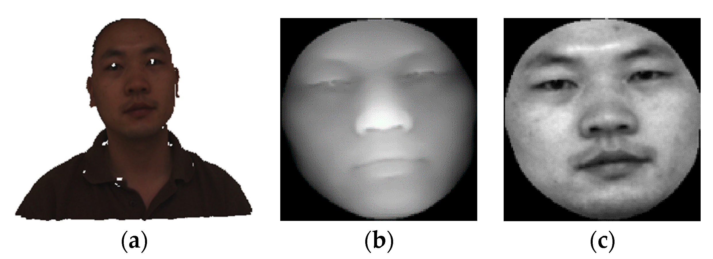
The bimodal maps obtained from 3D face point cloud model. (a) Example of 3D face data model in CASIA database; (b) example of the depth map; (c) example of the intensity map.
Figure 2.
The bimodal maps obtained from 3D face point cloud model. (a) Example of 3D face data model in CASIA database; (b) example of the depth map; (c) example of the intensity map.

Figure 3.
Multiscale operation.
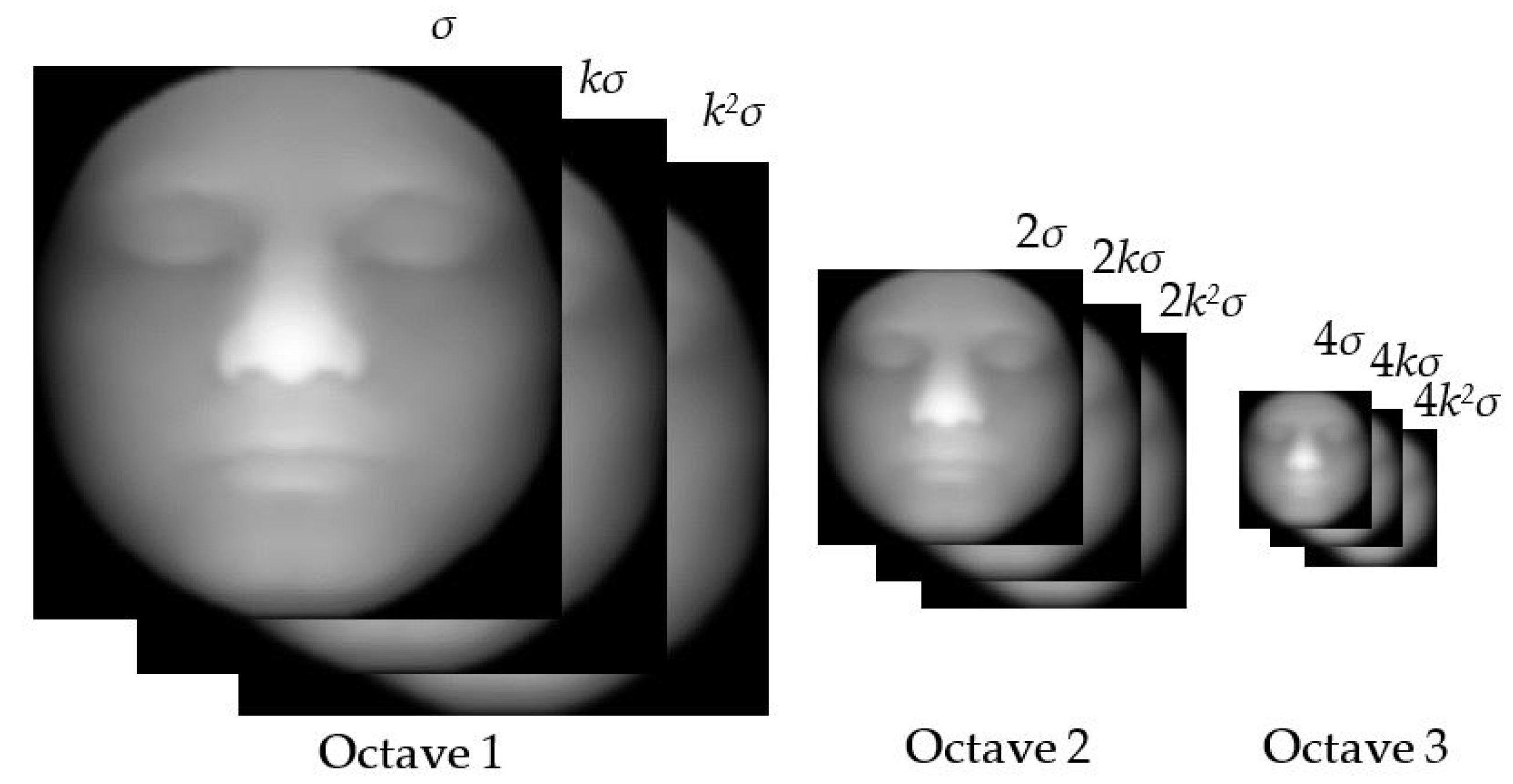
Figure 4.
Sub-blocks’ operation: (a) The original depth map; (b) 2 × 2 sub-blocks image; (c) 4 × 4 sub-blocks image; (d) 8 × 8 sub-blocks image; (e) 16 × 16 sub-blocks image.
Figure 4.
Sub-blocks’ operation: (a) The original depth map; (b) 2 × 2 sub-blocks image; (c) 4 × 4 sub-blocks image; (d) 8 × 8 sub-blocks image; (e) 16 × 16 sub-blocks image.

Figure 5.
Kirsch masks.
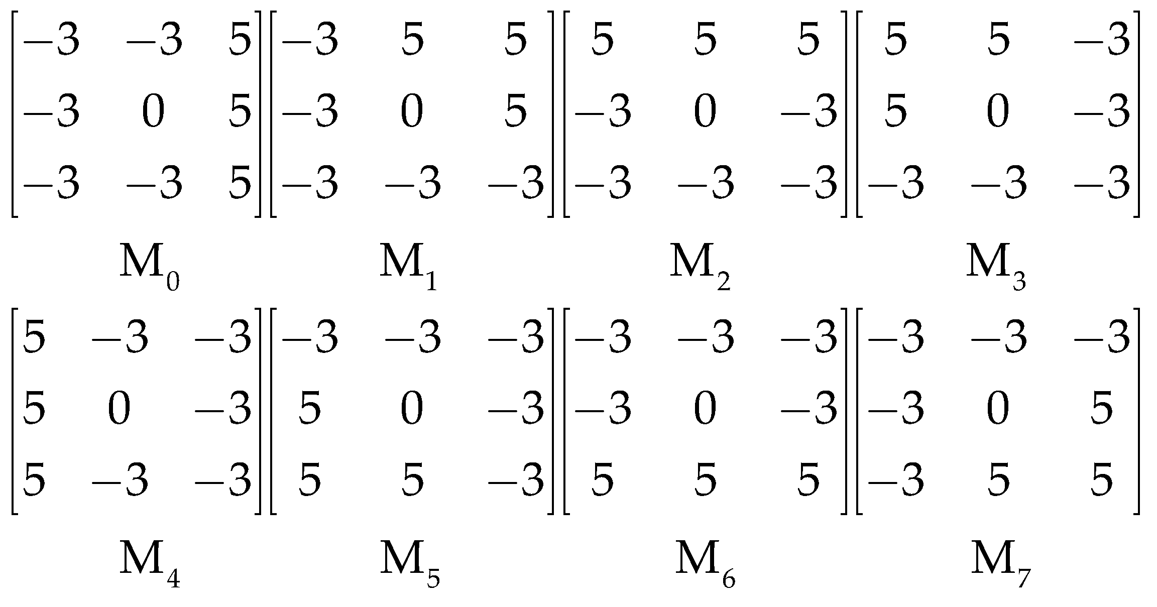
Figure 6.
Directions of the gradients. (a) The four different directions of relative gradients in GBP; (b) The eight different directions of relative gradients in LGP.
Figure 6.
Directions of the gradients. (a) The four different directions of relative gradients in GBP; (b) The eight different directions of relative gradients in LGP.
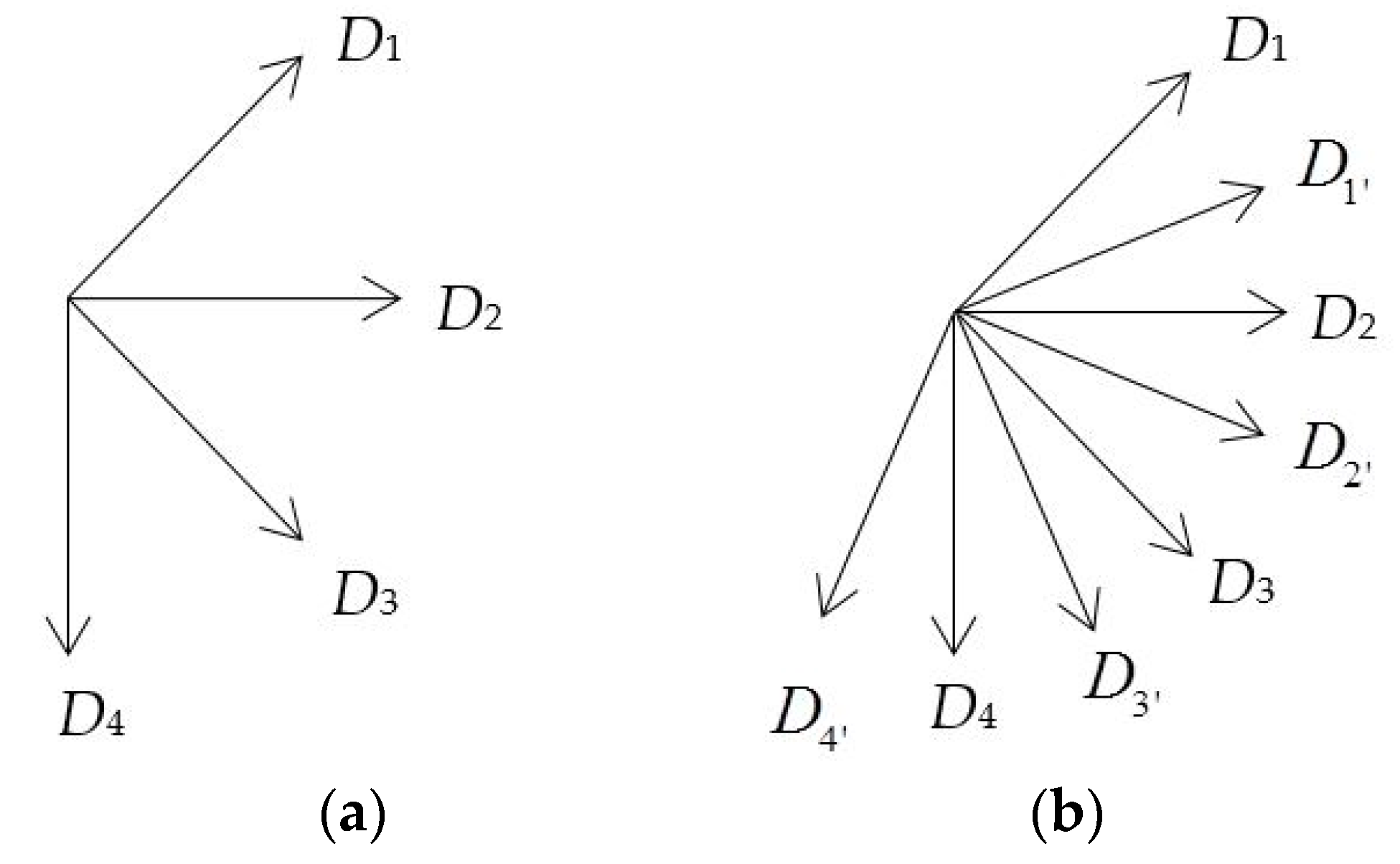
Figure 7.
Eight directional masks.

Figure 8.
Local gradient pattern (LGP) encoding process.
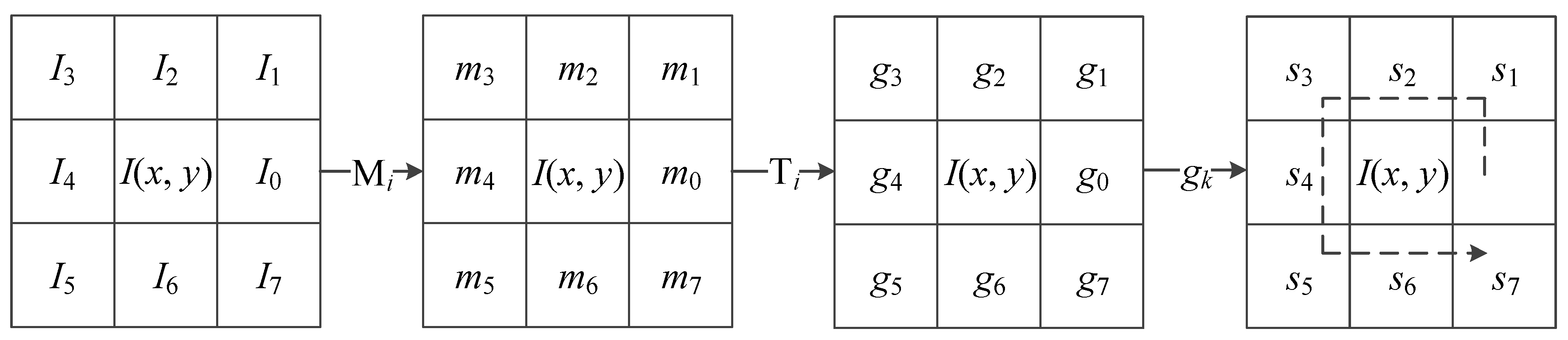
Figure 9.
LGP encoding example with k = 3.

Figure 10.
Samples of the CASIA database: (a) 18 depth map samples; (b) 18 intensity map samples.

Figure 11.
Samples of the FRGC v2.0 database: (a) nine depth map samples; (b) nine intensity map samples.
Figure 11.
Samples of the FRGC v2.0 database: (a) nine depth map samples; (b) nine intensity map samples.

Figure 12.
Samples of the Bosphorus database. (a) 40 depth map samples; (b) 40 intensity map samples.
Figure 12.
Samples of the Bosphorus database. (a) 40 depth map samples; (b) 40 intensity map samples.
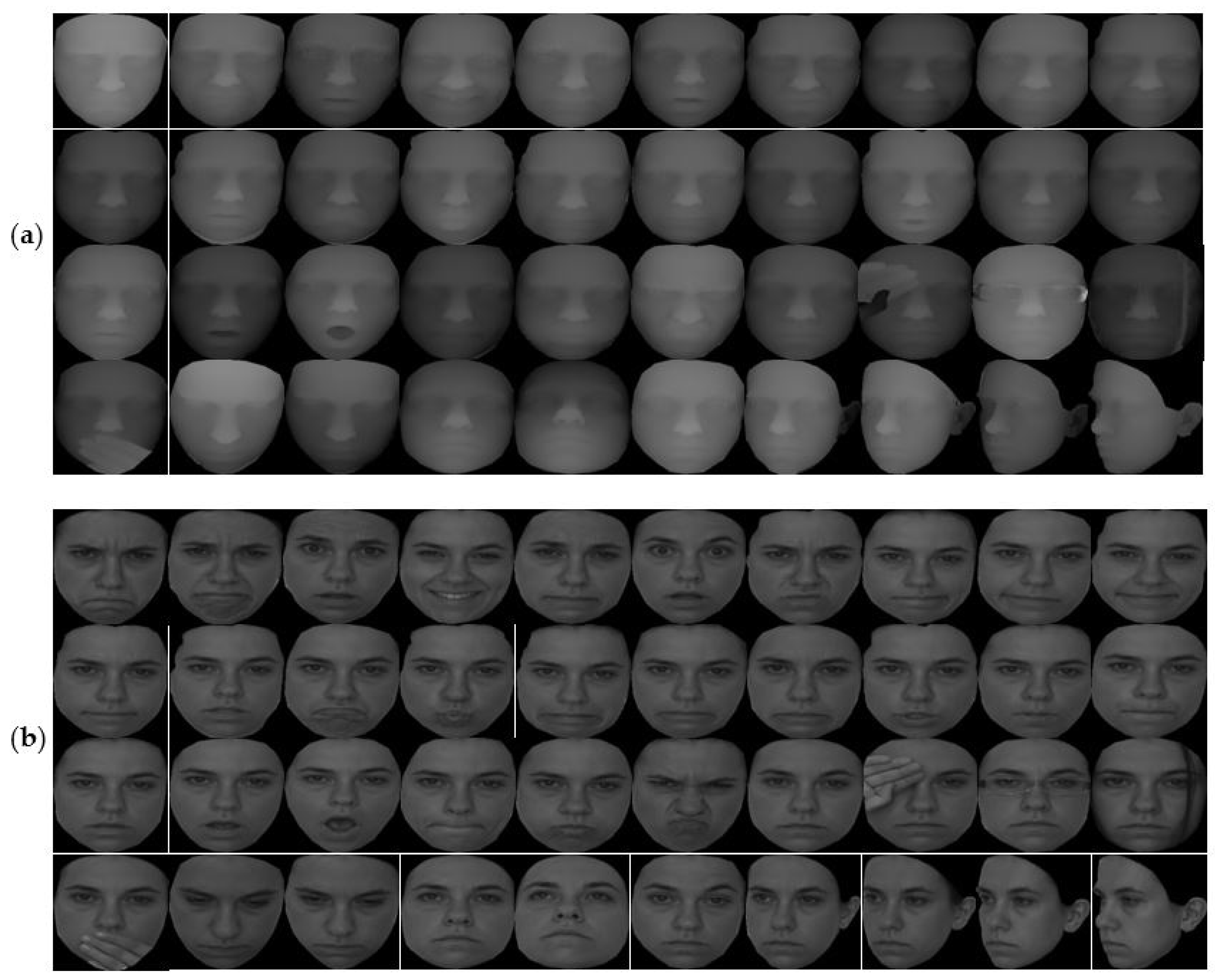
Figure 13.
Maps of the five descriptors: local binary pattern (LBP), local directional pattern (LDP), gradient binary pattern (GBP), LGP and weighted histogram of gradient orientation (WHGO). (a) The original depth map and intensity map; (b) corresponding LBP maps; (c) corresponding LDP maps; (d) corresponding GBP maps; (e) corresponding LGP maps; (f) corresponding WHGO maps.
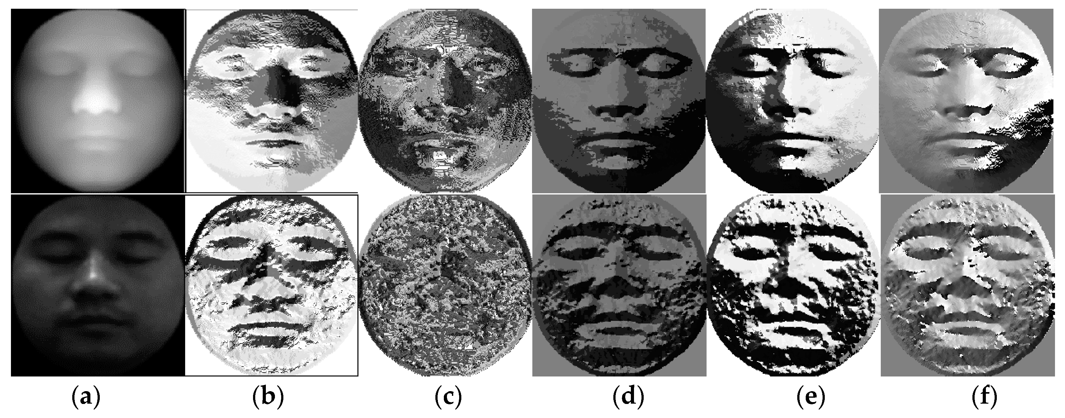
Figure 14.
Comparison of the LGP, WHGO, and three other descriptors: (a) the results of the LBP descriptor; (b) the results of the LDP descriptor; (c) the results of the GBP descriptor; (d) the results of the LGP descriptor; (e) the results of the WHGO descriptor. Abscissa: gradient orientation after being quantized; Ordinate: weighted frequency value.


Table 1.
Recognition rate comparisons of the five descriptors from the CASIA database.
| Descriptor | Image Type | STr/STe/RR (%) | STr/STe/RR (%) |
|---|---|---|---|
| LBP [28] | DM + IM | 360 + 360/360 + 360/95.56 | 720 + 720/720 + 720/94.17 |
| LDP [27] | DM + IM | 360 + 360/360 + 360/83.33 | 720 + 720/720 + 720/83.19 |
| GBP [26] | DM + IM | 360 + 360/360 + 360/95.83 | 720 + 720/720 + 720/94.03 |
| LGP | DM + IM | 360 + 360/360 + 360/96.67 | 720 + 720/720 + 720/96.53 |
| WHGO [26] | DM + IM | 360 + 360/360 + 360/94.44 | 720 + 720/720 + 720/94.31 |
Table 2.
Recognition rate comparisons of the five descriptors from the FRGC v2.0 database.
| Descriptor | Image Type | STr/STe/RR (%) | STr/STe/RR (%) |
|---|---|---|---|
| LBP [28] | DM + IM | 360 + 360/360 + 360/96.39 | 720 + 720/720 + 720/94.31 |
| LDP [27] | DM + IM | 360 + 360/360 + 360/91.67 | 720 + 720/720 + 720/92.36 |
| GBP [26] | DM + IM | 360 + 360/360 + 360/96.67 | 720 + 720/720 + 720/95.00 |
| LGP | DM + IM | 360 + 360/360 + 360/96.94 | 720 + 720/720 + 720/95.28 |
| WHGO [26] | DM + IM | 360 + 360/360 + 360/94.44 | 720 + 720/720 + 720/92.50 |
Table 3.
Recognition rate comparisons of the five descriptors from the Bosphorus database.
| Descriptor | Image Type | STr/STe/RR (%) | STr/STe/RR (%) |
|---|---|---|---|
| LBP [28] | DM + IM | 800 + 800/800 + 800/94.00 | 1600 + 1600/1600 + 1600/93.63 |
| LDP [27] | DM + IM | 800 + 800/800 + 800/81.25 | 1600 + 1600/1600 + 1600/81.31 |
| GBP [26] | DM + IM | 800 + 800/800 + 800/94.25 | 1600 + 1600/1600 + 1600/93.25 |
| LGP | DM + IM | 800 + 800/800 + 800/95.00 | 1600 + 1600/1600 + 1600/94.20 |
| WHGO [26] | DM + IM | 800 + 800/800 + 800/93.00 | 1600 + 1600/1600 + 1600/93.13 |
Table 4.
Recognition rates from the CASIA database using different descriptors combined with WHGO.
| Descriptor | Image Type | STr/STe/RR (%) | STr/STe/RR (%) |
|---|---|---|---|
| LBP-WHGO | DM + IM | 360 + 360/360 + 360/97.50 | 720 + 720/720 + 720/97.64 |
| LDP-WHGO | DM + IM | 360 + 360/360 + 360/94.72 | 720 + 720/720 + 720/93.61 |
| GBP-WHGO | DM + IM | 360 + 360/360 + 360/98.06 | 720 + 720/720 + 720/97.78 |
| LGP-WHGO | DM + IM | 360 + 360/360 + 360/98.60 | 720 + 720/720 + 720/98.47 |
Table 5.
Recognition rates from the FRGC v2.0 database using different descriptors combined with WHGO.
Table 5.
Recognition rates from the FRGC v2.0 database using different descriptors combined with WHGO.
| Descriptor | Image Type | STr/STe/RR (%) | STr/STe/RR (%) |
|---|---|---|---|
| LBP-WHGO | DM + IM | 360 + 360/360 + 360/97.78 | 720 + 720/720 + 720/96.53 |
| LDP-WHGO | DM + IM | 360 + 360/360 + 360/93.89 | 720 + 720/720 + 720/93.47 |
| GBP-WHGO | DM + IM | 360 + 360/360 + 360/96.94 | 720 + 720/720 + 720/96.11 |
| LGP-WHGO | DM + IM | 360 + 360/360 + 360/98.06 | 720 + 720/720 + 720/96.94 |
Table 6.
Recognition rates from the Bosphorus database using different descriptors combined with WHGO.
Table 6.
Recognition rates from the Bosphorus database using different descriptors combined with WHGO.
| Descriptor | Image Type | STr/STe/RR (%) | STr/STe/RR (%) |
|---|---|---|---|
| LBP-WHGO | DM + IM | 800 + 800/800 + 800/94.75 | 1600 + 1600/1600 + 1600/94.19 |
| LDP-WHGO | DM + IM | 800 + 800/800 + 800/88.50 | 1600 + 1600/1600 + 1600/87.56 |
| GBP-WHGO | DM + IM | 800 + 800/800 + 800/96.37 | 1600 + 1600/1600 + 1600/94.94 |
| LGP-WHGO | DM + IM | 800 + 800/800 + 800/96.75 | 1600 + 1600/1600 + 1600/96.44 |
Table 7.
Comparison of recognition rates using the CASIA database.
| Method | STr | STe | RR (%) |
|---|---|---|---|
| FNN-VRL [2] | 25 | 17 | 98.90 |
| SLF+LBP+SIFT [18] | 500 | 400 | 97.22 |
| MPCA+MDA [19] | 943 | 4007 | 97.53 |
| LGP-WHGO | 720 | 720 | 98.61 |
© 2018 by the authors. Licensee MDPI, Basel, Switzerland. This article is an open access article distributed under the terms and conditions of the Creative Commons Attribution (CC BY) license (http://creativecommons.org/licenses/by/4.0/).
Share and Cite
MDPI and ACS Style
Guo, Y.; Wei, R.; Liu, Y. Weighted Gradient Feature Extraction Based on Multiscale Sub-Blocks for 3D Facial Recognition in Bimodal Images. Information 2018, 9, 48. https://doi.org/10.3390/info9030048
AMA Style
Guo Y, Wei R, Liu Y. Weighted Gradient Feature Extraction Based on Multiscale Sub-Blocks for 3D Facial Recognition in Bimodal Images. Information. 2018; 9(3):48. https://doi.org/10.3390/info9030048
Chicago/Turabian StyleGuo, Yingchun, Ruoyu Wei, and Yi Liu. 2018. "Weighted Gradient Feature Extraction Based on Multiscale Sub-Blocks for 3D Facial Recognition in Bimodal Images" Information 9, no. 3: 48. https://doi.org/10.3390/info9030048
Note that from the first issue of 2016, this journal uses article numbers instead of page numbers. See further details here.