Calibration of C-Logit-Based SUE Route Choice Model Using Mobile Phone Data

1
Faculty of Maritime and Transportation, Ningbo University, Ningbo 315211, China
2
National Traffic Management Engineering & Technology Research Center Ningbo University Sub-Center, Ningbo 315211, China
3
Jiangsu Province Collaborative Innovation Center for Modern Urban Traffic Technologies, Nanjing 210096, China
*
Author to whom correspondence should be addressed.
Information 2018, 9(5), 115; https://doi.org/10.3390/info9050115
Submission received: 18 March 2018
/
Revised: 27 April 2018
/
Accepted: 6 May 2018
/
Published: 8 May 2018
Abstract
:Theoretically speaking, the data of a stated preference survey could be suggested for the calibration of a stochastic route choice model. However, it is unrealistic to implement the questionnaire survey for such a large number of alternative routes. Engineers generally determine the parameter empirically. This experienced choice of perception parameter may cause higher errors in the route flows. In our calibration model of the perception parameter, the data of the cellular network is set as the input. This model consists of two levels. The upper level is to minimize the gap squares of the route choice ratio between the C-logit model and the cellular network data. The stochastic user equilibrium (SUE) in terms of the C-logit model is used as the lower level. The simulated annealing (SA) algorithm is used to solve the model, where the route-based gradient projection (GP) algorithm is used to solve the inner SUE. A case study is used to validate the convergence of the model calibration. A real-world road network is used to demonstrate the objective advantage of an equilibrium constraint over a nonequilibrium constraint and explain the feasibility of the candidate routes assumption.
1. Introduction
The traffic conditions on a road network under continuous change from minute to minute, and it is hard for travelers to forecast the traffic in the future or understand the real-time traffic situation. This situation of incomplete information results in the stochastic perceptions in the travel costs for the travelers. Stochastic choice models are widely used to describe people’s route choice behavior. These models are used to solve the problem of finding link (route) flows on a given traffic network between the origins and the destinations. If an extra assumption that no driver can improve his/her perceived travel time by unilaterally changing routes is added, it becomes a stochastic user equilibrium (SUE) assignment problem.
A stochastic route choice model requires a random variable representing the error term being determined, i.e., the difference between the perceived travel time and the actual one. The Gumbel distribution and multivariate normal distribution have been tested as the distributions of the random variable in the logit and the probit route choice model. The logit-based model has been more widely tested by researchers due to its relatively low computational complexity.
The independence of irrelevant alternatives (IIA) is an assumption in the general multinomial logit (MNL) model. This means that if a route is added into a candidate set, the IIA feature simply assumes that this route has no common links with pre-existing routes. In most cases, overlaps in parts of the routes are common. For this reason, many researchers developed improved logit models such as C-logit, nested logit, path size logit, etc. [1,2,3], and the C-logit model is accepted widely due to its simplicity [4].
As to the C-logit-based SUE model, the variance of the random variable is indicated by the perception parameter θ of the error term. It is an essential parameter in these models since it scales the error term and describes the accuracy of the perceived travel time. Therefore, this parameter of the error term can have a significant impact on the road flow results.
In the calibration of this perception parameter, most researchers have realized that the general maximum likelihood approach is invalid because the number of route alternatives is large and the stated preference survey is difficult to be implemented. Therefore, the parameter value is determined empirically in most applications. Engineers generally select several numbers for each neighbor with equal gaps first. These numbers are taken as parameter value candidates. The best fit value is determined by testing the routing choice results of several origin–destination (OD) pairs. Only a few researchers have discussed the process of an optimization model to set this parameter. One suggested using a least squares approach in the calibration [5], given the route and link flows. They set the minimization of the gap square between the real-world route choice ratio and the model-based ratio as the objective, while the MNL-based SUE model was set as the constraint. Again, a common link problem was not considered in the proposed method and the given route flows were difficult to obtain through a traditional traffic field investigation.
Flows of routes or aggregated routes are the basic data for SUE model calibration. The collection of the data is a significant issue. In the age of big data, the spatial–temporal positioning data of cell phones are related to route flows and may be an effective data source in calibrating a C-logit-based SUE model.
The GPS data of cell phones are more likely to be used in the problem of travel route choice. Previous route choice analysis with GPS data was focused on map matching (MM). MM algorithms are generally used to infer from GPS data based on the corresponding elements in the transportation network, including locations, links, and paths. A comprehensive review of 35 MM algorithms for navigation applications since 1989 was presented by Quddus et al. (2007) [6]. Most MM algorithms are designed to conduct point-to-point matching by detecting the correct link for each GPS point. However, the closest edge or shape point is not guaranteed to be the correct one, especially in urban road networks with a high density in small regions. Recent studies on MM focus not only on the localization of GPS samples on a map, but also on the inference of the travel path (Schuessler et al. 2009 [7]; Bierlaire et al. 2010 [8]; Ozdemir et al. 2018 [9]). Schuessler et al. (2009) [7] calculated a score of dissimilarity between GPS points and arcs based on distance, speed, and/or heading difference. The authors matched a route via these scores. However, their method required a set of dense and accurate GPS data. As for the condition that sparse GPS samples are on the travel routes, Bierlaire et al. (2010) [8] and Ozdemir et al. (2018) [9] used a path size logit model and a hybrid hidden Markov model to solve the MM problem separately.
Our research uses base station identity (ID) positioning data to analyze the route choice, which is different from the GPS data. The tower data’s precision is not as high as GPS data. Every cell phone’s position is determined by its tower’s position. In this case, it is not possible to precisely determine the relationship between the route and the cell phone trajectory. The one-by-one route matching method is not suitable in this condition even though it is available in the route choice model with the GPS data. The authors deal with all the routes and cell phone data together. Technically, unlike the previous logit route choice model of maximizing the likelihood function, in the proposed method, the gap of the route choice results and the cell phone trajectory data were minimized to obtain the parameter of the route choice model.
The base station ID positioning method is generally used to determine the cellphone user’s position and time information. Each time when a mobile phone user enters/exits the signal coverage of a base station, the station ID will be recorded together with the timestamp. A series of base station IDs and timestamps represent the user’s trip in terms of his or her phone ID path. The ID path information has been used in the field of transportation, such as OD demand estimation [10], route flow calculation [11], and link density analysis [12]. More recently, some new applications have been developed. For instance, Jiang et al. (2017) [13] used cellphone data to develop an activity-based model in generating an overall daily activity pattern.
Recently, researchers explored the relationship between road routes and ID paths. Chiou et al. (2015) [14] investigated the travel time for each road route and ID path. The authors used a minimum gap to make the matching work. Leontiadis et al. (2014) [15] proposed a more refined method to conduct matching. First, the authors considered the map as an aggregation of 15 × 15 m grids. Then, by calculating the association probabilities among the grids, road links, and ID stations, they applied the A-star algorithm to find the best matched routes.
The above route-matching studies with base station ID paths take road routes as the reference; all ID paths are projected onto these road routes. In this paper, the authors developed a reverse process to conduct the matching work, in which the ID path was the reference and the road routes were to be aggregated. By taking the driver’s stochastic route-choice behavior into account, the relationship between the ID path and the road route was generated. This work provides an alternative for the matching work of an ID path and a road route. On the other hand, this work contributes to the perception parameter calibration of a C-logit route choice SUE model with base station ID path data, which is quite different from the calibration of GPS data. Compared to GPS data, the base station ID path data have a lower positioning accuracy and a different positioning mechanism. Thus, in this paper, the authors embedded the ID path data and individual route data matching algorithm inside the bilevel model.
2. Methodology
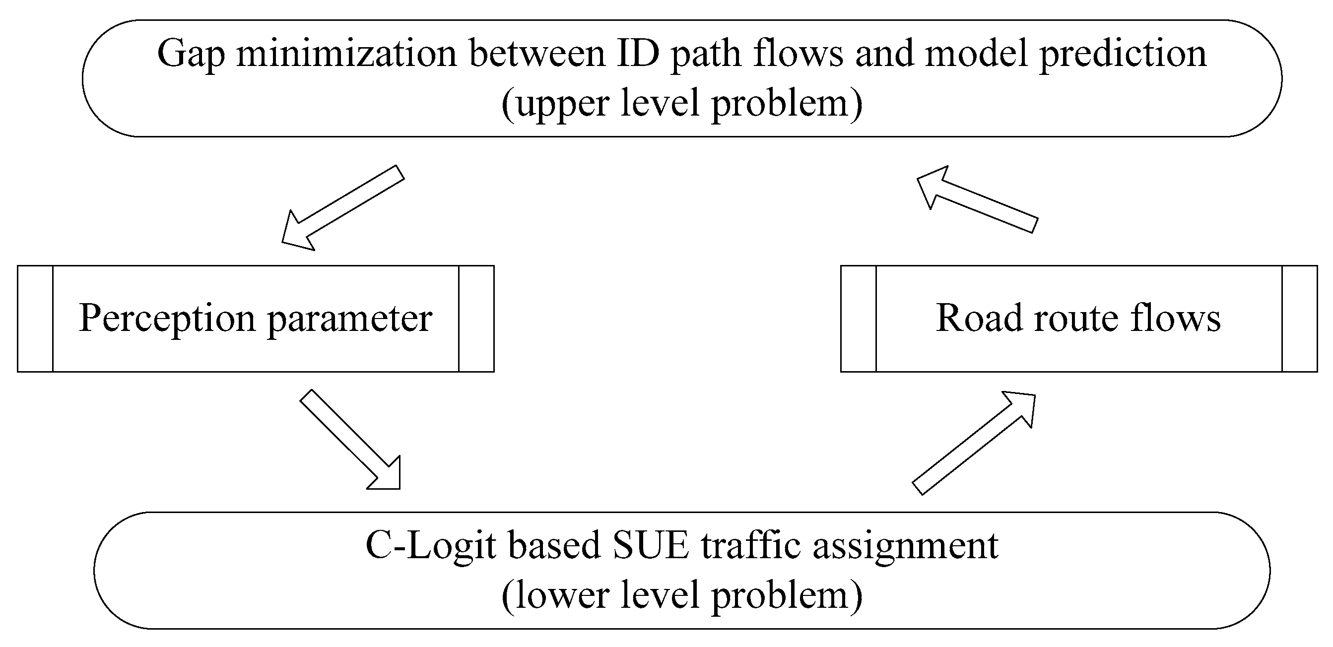
A bilevel optimization model was proposed to solve the interactive process between the perception parameter and the road flows. The process was in a top-down sequential manner. The lower level had the freedom to generate road flows within the broad range set of the top level. Furthermore, the output depended on the degree of interaction between the two levels, which were somewhat similar to the static two-person Stackelberg game. The interaction process of this parameter calibration problem was illustrated as Figure 1.
2.1. Model of Upper Level
Minimization of Flow-Ratio Gap Square
The C-logit route choice model shows the selection probability for the corresponding route. Equation (1) is the C-logit route choice model, in which is the selection probability for the road route r, θ is the perception parameter to be calibrated (it is a positive parameter, which is inversely proportional to the perception variance and describes the degree of dispersion of the network), and is a set of road routes for the given OD pair w.
Specifically, cr is the total travel cost for route r; its expression is as follows in Formula (2).
where A is the set of all road links. is the dummy variable of the relation between link a and travel route r (1, related; 0, otherwise). is the travel time of link a, and it can be calculated by the BPR (Bureau of Public Road) function shown in Formula (3).
where is the free-flow travel time of link a. is the capacity of link a. is the flow of link a. Assuming R is the route set, could be changed into the expression of route flow hr.
In Formula (2), is the common factor for travel route r. The calculation of is as follows. In Formula (5), is the length of the travel route r; is the overlapped length of l and r, and β is a parameter. If this parameter is equal to zero, the C-logit collapses to the MNL route choice model. If this parameter is equal to 1, the C-logit choice probabilities in the limiting case of N coincident paths tend to be 1/N of those calculated with an MNL model applied when considering the coincident paths as a single path. In this article, we assume that β is equal to 1 for all OD pairs.
Our aim is to minimize the flow-ratio difference between the aggregated routes and the corresponding ID path. This objective function for the θ calibration model is as follows.
where e represents the path of a base station antenna ID (it is a more refined ID that originated from base station ID). is a set of base station antenna ID paths for the OD pair w. is a specific set of road routes for OD pair w; these routes are inside the corresponding antenna signal coverages, and their moving direction is the same as that of the ID path e. is the share of the demand covered by the mobile phone path e versus the whole demand of the related OD pair ( can be obtained by analyzing the collected mobile phone data).
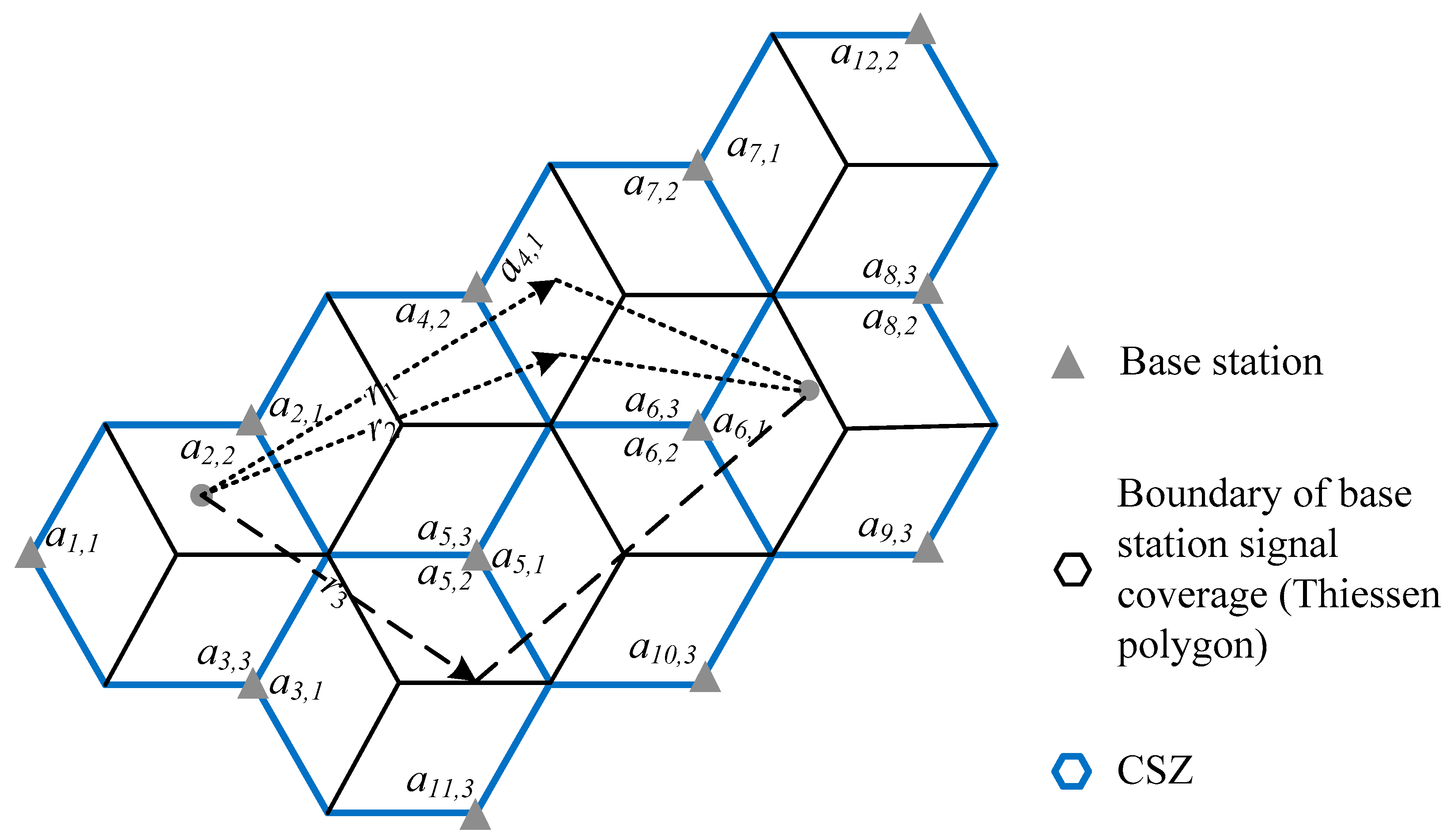
The relationship between the road route and the base station antenna ID path in the objective function was described in a small case (see Figure 2). Firstly, the authors explained the difference between the signal coverages of the base station and the base station antenna. The boundary of the base station signal coverage (Thiessen Polygon) is shown in a black hexagon in the figure, where the antenna signal of the corresponding base station could be received by users. As for the antenna signal, generally, one-directional antennas can only offer 120 degrees of coverage of signal. For the purposes of an omnidirectional coverage, there were three antennas for each base station. The signal coverage of different directional antennas in the neighbor base stations generally formed hexagons. Its boundaries are shown in blue hexagons in the figure. Each hexagon is covered by three antennas of three base stations nearby, and each hexagon is thus named as the common signal zone (CSZ). The variable was used to represent the location ID for the directional antenna j in the base station i. This zone is an overlapping part of the Thiessen polygon and the CSZ. In this article, the authors assumed that each zone of the location ID represented a traffic analysis zone (TAZ). Variable was used to represent this zone. It is easy to collect zone ID from mobile phone data, so the base station antenna ID path was directly defined as follows: a set of TAZs constitutes the path of a base station antenna. For the purposes of convenience, the name ID path was used to represent the meaning of the base station antenna ID path in this article.
For a given OD pair w ( to ), the road route set was assumed to consist of , , and . It can be seen in Figure 2 that the travel routes and can be matched up to the same ID path , and the travel route can be matched up to . If the shared portion of the collected demand for the ID path is P1, while is P2, then the θ calibration model of Formula (6) can be changed to a special style:
2.2. Model of Lower Level
(1) Unbalanced condition
If we only consider the unbalanced condition, it means that the perceived travel time is not related to link flows. The upper level model can obtain the variable θ directly. Thus, we should not construct the lower level model. Furthermore, we can use the following C-logit model to calculate the route flow.
where is the total travel demand of the OD pair w.
(2) Balanced condition
Function (9) is the SUE in terms of the C-logit model, and thus it also becomes the lower level model of θ calibration.
Formula (9) is a function of route flow, and it is also known as Fisk’s SUE model. Fortunately, only one constraint is included in this model, and this constraint is that route flow must not be less than zero. Fisk’s SUE model is a strictly convex programming problem and has an optimal route flow solution .
3. Solution Algorithms
The complexity of the above problem is similar to the traffic network design problem. It is also a Non-deterministic Polynomial problem, and the heuristic method is a common approach to this kind of problem. According to previous research [16], many researchers use the genetic algorithm (GA) and the simulated annealing (SA) algorithm. It is noted that when the variable is continuous such as in continuous network design problems, the application of SA is higher because its performance is better in this condition [16]. The reason is that the SA is less sensitive to the size of the solution space when compared to other methods such as the GA. In this article, since the variable is continuous, the SA is adopted.
3.1. Adopted SA Algorithm
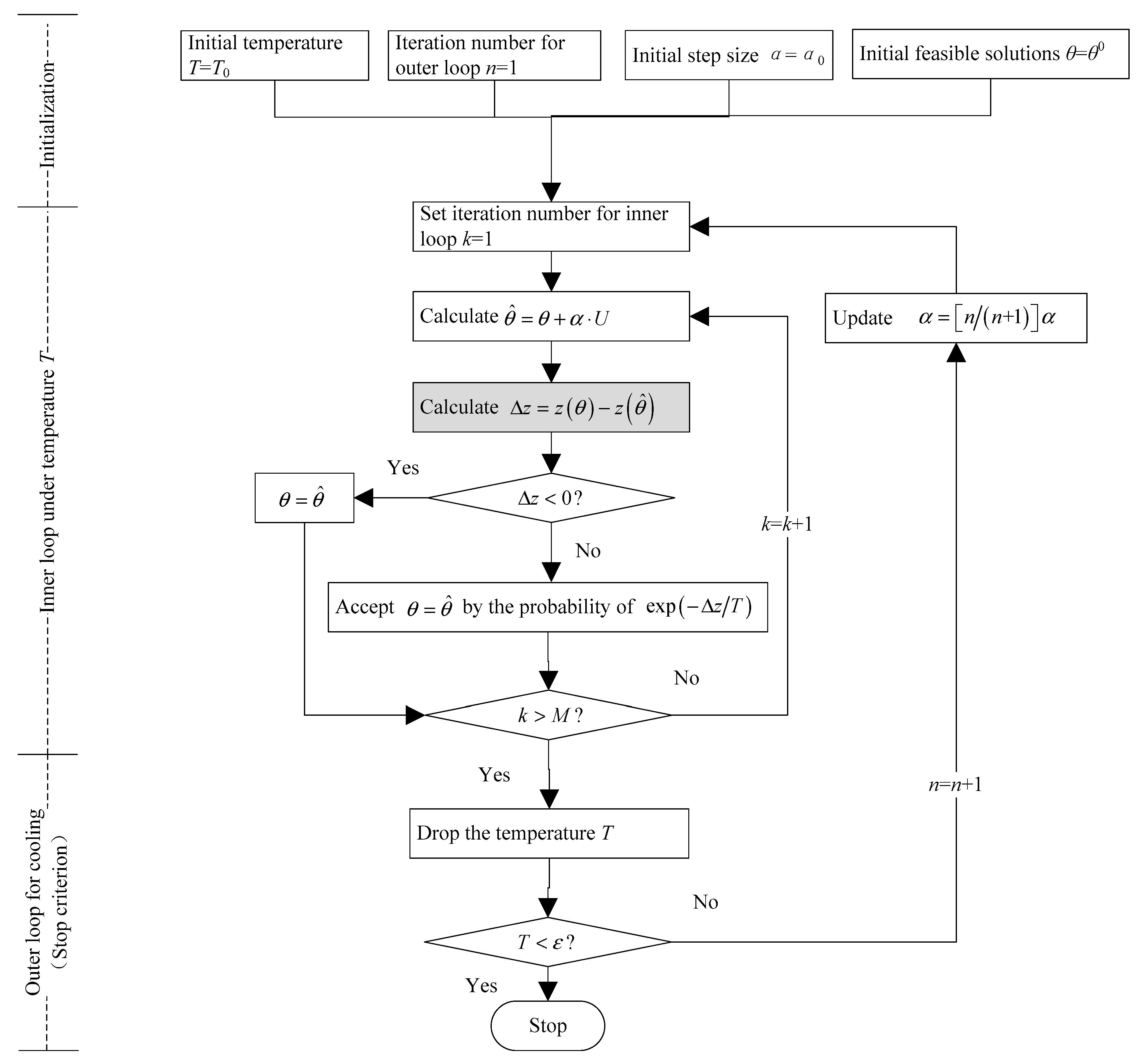
The SA is a probabilistic technique for approximating the global optimum of a function. It comes from annealing in metallurgy, a technique that involves the heating and the controlled cooling of a material to increase the size of its crystals and to reduce their defects. Initially, a high temperature is set. As the temperature decreases in each step, the change of the objective function Δz is evaluated. If the new solution can generate a better objective value, the solution will be accepted. Otherwise, the solution will be accepted conditionally with the possibility of , in which T is the related temperature in that state. The conditional acceptance of inferior solutions enables the SA to avoid local optima. The SA repeats M times at each controlled temperature to achieve a heat balance. The M is a control parameter, which is also known as the Markov length. The above step is repeated until a given computational budget has been exhausted.
Figure 3 shows the flowchart for the proposed SA. It is obvious that there are two feedback loops. In the outer cooling loop, if the number of iterations n ≥ 12, then temperature T = 0.5T and n = n + 1; otherwise, T = 0.8T, n = n + 1, and the algorithm will return to the inner loop. In the proposed algorithm, the temperatures in the consecutive two iterations are different for pre-stage and post-stage iterations. T would decrease slowly in the pre-stage iteration but would drop quickly in the post-stage iteration, which could increase the probability of escaping from the local optimum in the pre-stage iteration. When iterations of the decision variable θ in the inner loop are conducted, the related random variable U follows a uniform distribution in the range .
3.2. Objective Function Calculation Inside SA Algorithm
The procedures for the calculation of the objective function for the given θ in the SA are as follows: first, the SUE model is solved by using the gradient projection (GP) method, and the route flows are then obtained. Based on the route flows, the travel costs in the objective function are updated and an objective function value in the grey box of Figure 3 is achieved.
In Fisk’s SUE model, the total route cost is not simply an accumulation of the link cost ; therefore, there is a need for a route-based method rather than a general traffic assignment method to solve this problem [17]. The GP method is a route-based method, and thus it was chosen. Another reason for adopting the GP method is that it is a requirement of the nonzero constraint for the route flow. If the superior solution of a certain iteration is not in the feasible solution space, the GP method can lead to a superior solution to be orthogonally projected into the feasible solution space. The orthogonally projected vector would be in a non-obtuse angle relation with the steepest descent vector; therefore, the GP algorithm is a feasible direction method. The GP algorithm is as follows:
Step 1: Initialization
Use the C-logit model to assign the initial route flow and update the initial link flow , then set up the convergence threshold φ and iteration m = 0;
Step 2: Update of the costs of link and route
Use as the input data to update the link travel cost ; use to update the mapping , which is the derivative of the objective Function (9) with respect to ;
Step 3: Search of the reference routes
Search the reference routes for the OD pair w based on ;
Step 4: Projection of route flow
Use the following formula to calculate the non-reference route flow:
Update non-reference and reference route flows:
Update the link flow based on the conservation between link and route flows;
Step 5: Stop criteria
If , exit ( is total route number); otherwise, m = m + 1, return to Step 2.
The GP algorithm selects the reference route per iteration according to the following criterion: the unit increase of flow results in the minimum increase in the objective function value. Other routes are chosen to be the non-reference routes. In other words, the reference route is the best search direction in the feasible solution space. The flow in the non-reference route is transferred to the reference route. To ensure that the transferred route flow vector is not negative, the negative vectors will be automatically set to be zero. To prove that the transferred is the orthogonal projection of the original vector in the feasible solution space, we will explain this as follows. Assume that there is a full space vector , and is its orthogonal projection vector in the feasible solution space. Then, the sufficient and necessary conditions () should be satisfied according to the GP principle. in this condition is the arbitrary vector in the feasible solution space. The above condition for and indicates that the orthogonally projected vector has the closest distance to the original vector. In our route-flow searching case, the non-negative space is set as the feasible solution space. We set the negative elements in to be zero to ensure that the converted is the one that is the closest to the primary . This operation can accurately make the converted equal to such that the orthogonal procession is workable.
4. Case Study
4.1. Small-Sized Network
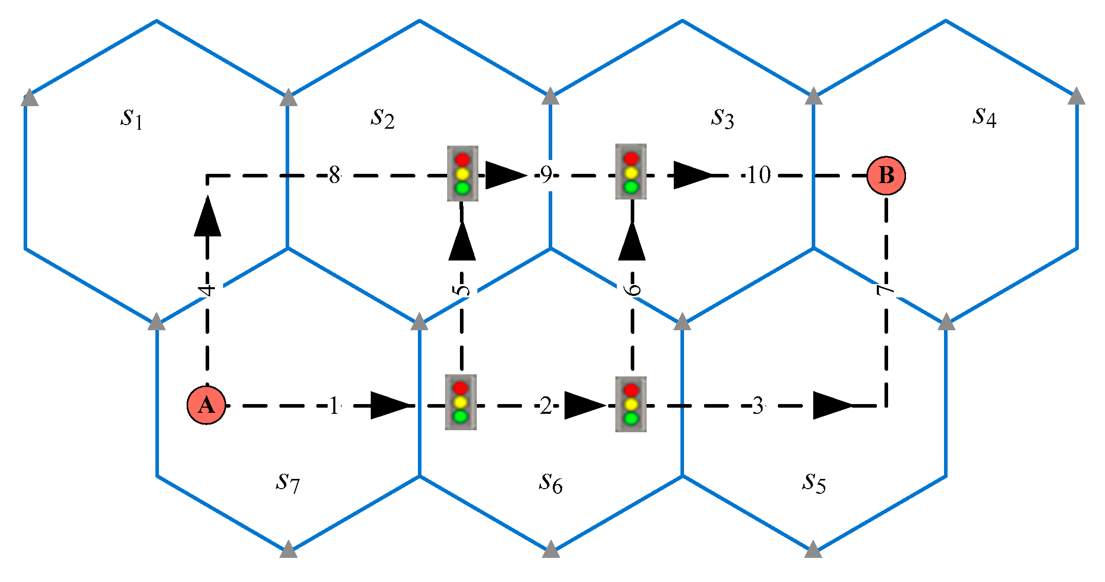
Figure 4 is a model convergence illustration of a small-sized network. Four alternative routes from A to B are listed in Table 1. The travel route and the ID path is in a one-to-one relation. The collected demands for the four ID paths are (240, 230, 215, 210) vehicles per hour. The free flow travel time for each link is (2, 2, 0.5, 3, 4, 2, 0.5, 4, 2, 1) min, so the total travel time for the four routes is (5, 7, 9, 10) min. Assume that the parameter = 1. Assume that the link travel time is independent to the link flow, so the θ calibration model becomes a one-variable model without any constraints. This case uses a simple golden selection method to solve the parameter. The convergence criterion for the error is 0.001. The last three steps of the method are listed in Table 2. θ is 0.0274, which is the average value at the last iteration. The objective value converged to 6.7367 × 10⁻⁶.
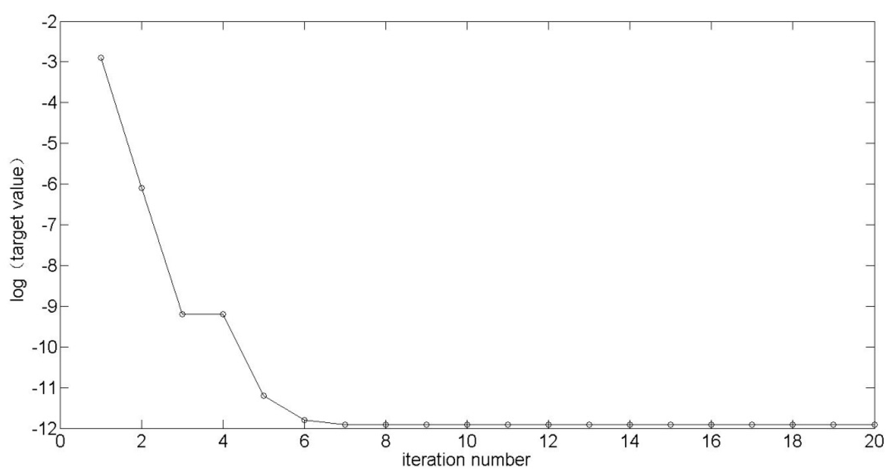
Figure 5 is the convergence of the objective value when using SA. When it is converged, the value in the longitudinal axis point is −11.9079. This value is the same as the logarithmic form of the objective value obtained in the golden selection method. It demonstrated the validity of SA in some sense.
If the assumption of an independent link cost is relaxed, the BPR function can be used to calculate link travel time. As for the BPR function, the multiplier and exponent parameters can be 0.15 and 4. The capacity of each link can be 1000 vehicles per hour. The final θ = 0.03 is obtained when the objective value reaches 1.3185 × 10⁻⁵. The demand and total travel costs for the four routes are shown in Table 3. It was observed that when the travel cost increased, the demand of the related route decreased accordingly. This corresponds with the rule of stochastic equilibrium.
4.2. Case Study for Urban Street Network
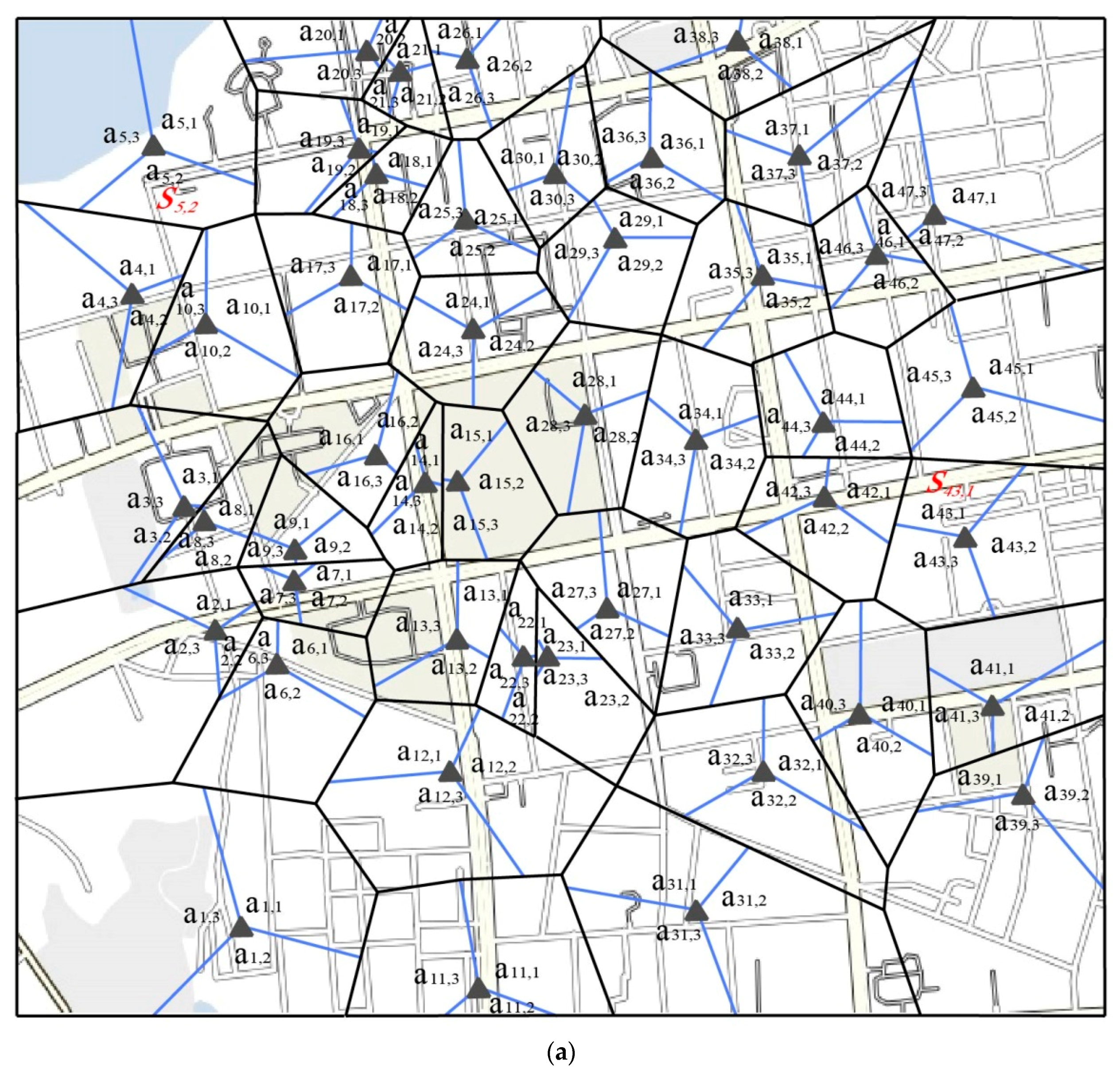
A data set on 23 December 2016 was obtained from the local telecommunications company for an urban area (Figure 6a). The data set includes call records, browsing records, and usage records of cellphone applications such as WeChat and QQ (Figure 6b). During the rush time window of 5:00 p.m.–6:00 p.m., there were 114.1 thousand records which were transferred into 10.9 thousand cellphone users’ paths. Firstly, an initial screening process was performed. Then, the ID paths were collected for use in the parameter calibration in the stochastic route choice model.
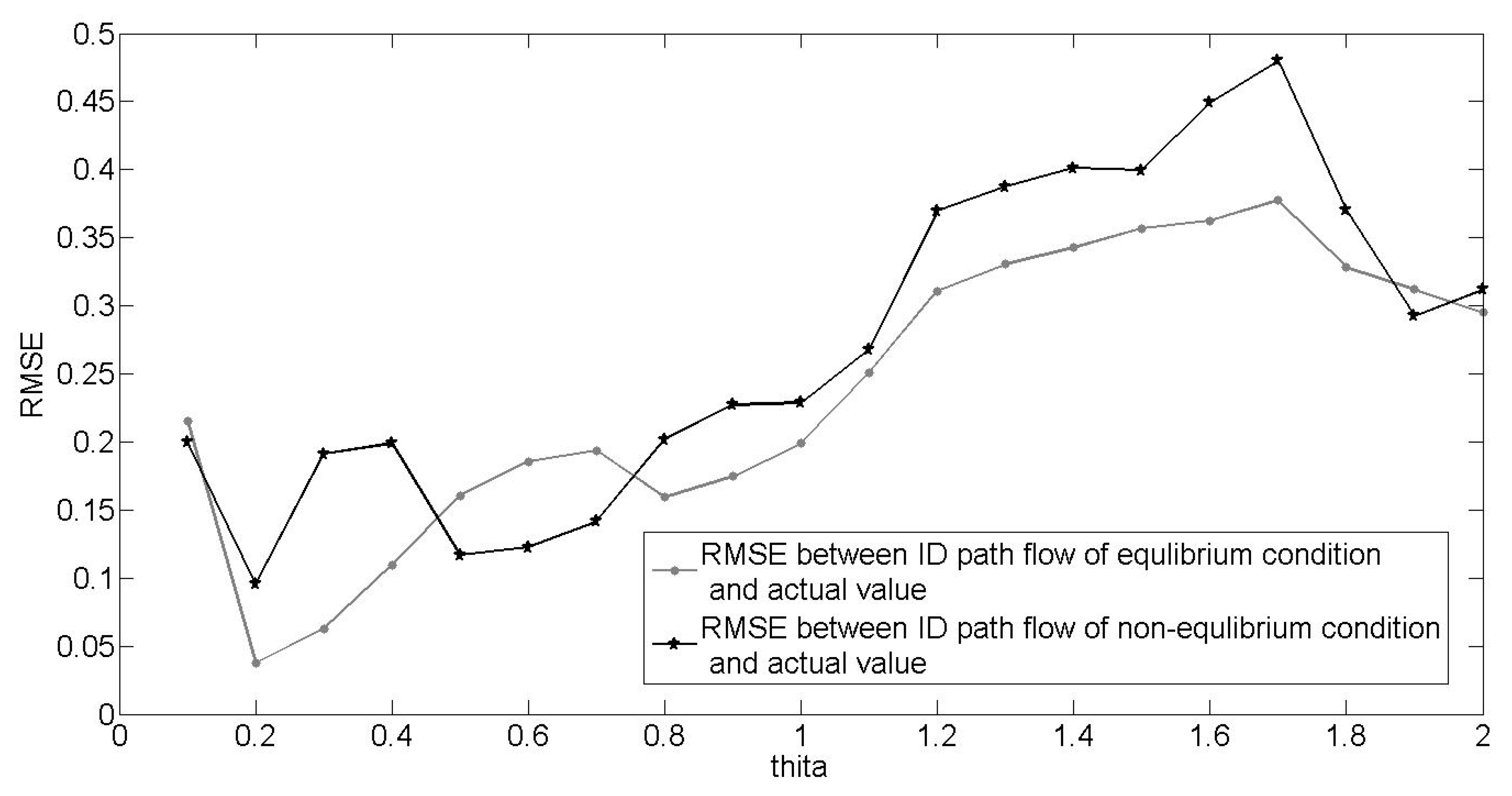
Figure 7 illustrates the difference between equilibrium and nonequilibrium assignments for a given θ. The Root Mean Square Error (RMSE) is the difference between the ID path flow inferred in reverse from the traffic assignment model and the data records from the telecommunication company. It was clear that the equilibrium assignment performed better than the nonequilibrium assignment in most of the RMSE results. Therefore, the equilibrium assignment model may be more realistic. Moreover, the optimal solution of the SA algorithm was obtained when θ = 0.23, which is also close to the result of enumeration in Figure 7.
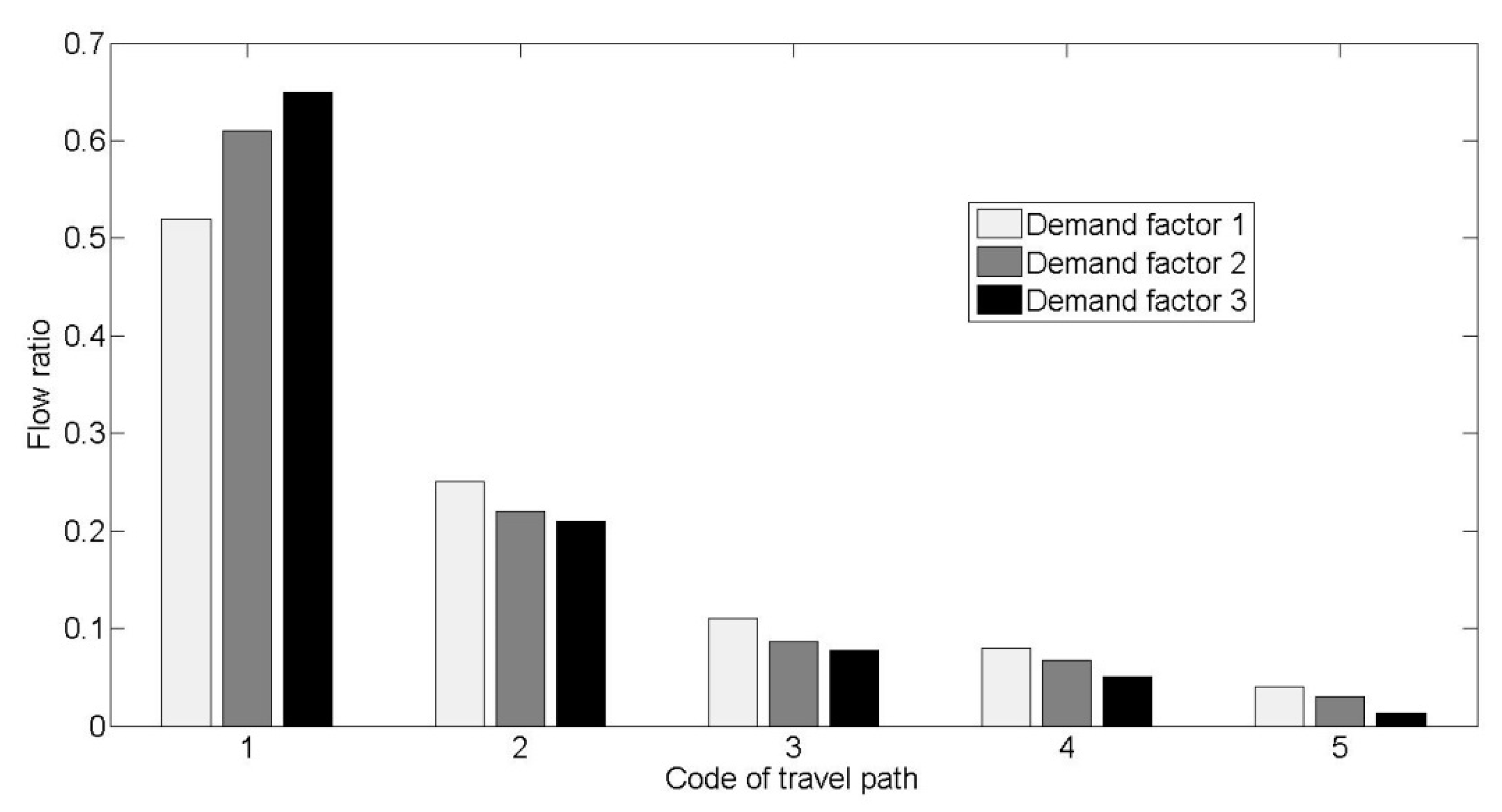
To effectively match the travel route and the ID path, the travel route set for each OD pair has already been generated in the initial step. The assignment of the travel route set follows these rules: (1) ensure each ID path has a related travel route; (2) the travel route set is developed based on the K-shortest path algorithm; and (3) the maximum number of route alternatives for an OD pair is less than 7. To validate the candidate-generation method, we analyze the route flow variation under the influence of demand variation between TAZs and . As is demonstrated in Figure 8, flows exist in all five candidate routes (the flow in the sixth alternative is very small so it is omitted in the figure). It is also observed that the variance of the flows in different alternatives is small under different demand factors, which means that the assumption of the limited number of alternatives is stable and could be feasible.
5. Conclusions
The contribution of this article is the application of mobile phone data in calibrating the C-logit-based SUE route choice model. This work can not only contribute to the perception parameter calibration of the route choice model, but also provide an alternative for the matching work of an ID path and a road route. The specific difference of the proposed model comes from the construction of the gap squared function, in which the flow of the base station antenna ID path was taken as the reference point and matched the covered road routes up to this cell phone trajectory. To validate the proposed model, two cases were discussed. The small case considered unbalanced and balanced conditions separately. The unbalanced condition corresponds to the one-level problem, whose precise result can be acquired by the golden selection method. The convergence procedure by the reference of precise results was shown. This case also took SUE as the constraint, and it obtained a feasible route flow. Another complex case was discussed in terms of a city’s network. The matching work between the phone data trajectory and the route was performed in this case, and the unbalanced and balanced conditions were tested. It is obvious that the equilibrium assignment performs better than the nonequilibrium in most RMSE results. Furthermore, the SUE constraints were considered to test the feasible number of candidate routes. The results revealed that five candidate routes are enough for candidate routes, and the assumption of the limited number of alternatives is stable and feasible. In the future, the proposed method will be applied to more urban areas to demonstrate its convergence and validity.
Author Contributions
Conceptualization: Z.H. and Z.H.; Writing—original draft: Z.H., Z.H. and W.X.; Writing—review & editing: P.Z.
Acknowledgments
This paper is partially supported by Zhejiang Provincial Natural Science Foundation of China (Y18E080041, LQ14E080002), Scientific Research Foundation for Returned Scholars, Ministry of Education of China (ZX2014000911), Zhejiang Social Science Planning Program of China (16NDJC015Z).
Conflicts of Interest
The authors declare no conflict of interest.
References
- Cascetta, E.; Nuzzolo, A.; Russo, F.; Vitetta, A. A modified logit route choice model overcoming path overlapping problems: Specification and some calibration results for interurban networks. In Proceedings of the 13th International Symposium on Transportation and Traffic Theory, Oxford, NY, USA, 24–26 June 1996; pp. 697–711. [Google Scholar]
- Bekhor, S.; Prashker, J. Stochastic user equilibrium formulation for generalized nested logit model. Transp. Res. Record J. Transp. Res. Board 2001, 1752, 84–90. [Google Scholar] [CrossRef]
- Ben-Akiva, M.; Bierlaire, M. Discrete choice methods and their applications to short term travel decisions. In Handbook of Transportation Science; Springer: New York, NY, USA, 1999; pp. 5–33. [Google Scholar]
- Xu, X.; Chen, A.; Zhou, Z.; Bekhor, S. Path-based algorithms to solve c-logit stochastic user equilibrium assignment problem. Transp. Res. Record J. Transp. Res. Board 2012, 2279, 21–30. [Google Scholar] [CrossRef]
- Zhang, X.; Rey, D.; Waller, S.T. Method of parameter calibration for error term in stochastic user equilibrium traffic assignment model. World Acad. Sci. Eng. Technol. Int. J. Math. Comput. Phys. Electr. Comput. Eng. 2014, 8, 1397–1403. [Google Scholar]
- Quddus, M.A.; Ochieng, W.Y.; Noland, R.B. Current map-matching algorithms for transport applications: State-of-the art and future research directions. Transp. Res. Part C Emerg. Technol. 2007, 15, 312–328. [Google Scholar] [CrossRef] [Green Version]
- Schuessler, N.; Axhausen, K.W. Processing Raw Data from Global Positioning Systems Without Additional Information. Transp. Res. Record J. Transp. Res. Board 2009, 2105, 28–36. [Google Scholar] [CrossRef]
- Bierlaire, M.; Chen, J.; Newman, J. Modeling Route Choice Behavior from Smartphone GPS data. In Proceedings of the 12th International Conference on Travel Behaviour Research, Jaipur, Rajasthan, India, 13–16 December 2009. [Google Scholar]
- Ozdemir, E.; Topcu, A.E.; Ozdemir, M.K. A hybrid HMM model for travel path inference with sparse GPS samples. Transportation 2018, 45, 233–246. [Google Scholar] [CrossRef]
- Iqbal, M.S.; Choudhury, C.F.; Wang, P.; González, M.C. Development of origin–destination matrices using mobile phone call data. Transp. Res. Part C Emerg. Technol. 2014, 40, 63–74. [Google Scholar] [CrossRef]
- Wu, C.; Thai, J.; Yadlowsky, S.; Pozdnoukhov, A.; Bayen, A. Cellpath: Fusion of cellular and traffic sensor data for route flow estimation via convex optimization. Transp. Res. Part C Emerg. Technol. 2015, 59, 111–128. [Google Scholar] [CrossRef]
- Yadlowsky, S.; Thai, J.; Wu, C.; Pozdnukhov, A.; Bayen, A. Link density inference from cellular infrastructure. In Proceedings of the Transportation Research Board (TRB) 94th Annual Meeting, Washington, DC, USA, 11–15 January 2014. [Google Scholar]
- Jiang, S.; Ferreira, J.; González, M.C. Activity-based human mobility patterns inferred from mobile phone data: A case study of Singapore. IEEE Trans. Big Data 2017, 3, 208–219. [Google Scholar] [CrossRef]
- Chiou, Y.C.; Hsieh, C.W. A virtual trip line matching model for cellular vehicle probe positioning and tracking. J. East. Asia Soc. Transp. Stud. 2015, 11, 1959–1969. [Google Scholar]
- Leontiadis, I.; Lima, A.; Kwak, H.; Stanojevic, R.; Wetherall, D.; Papagiannaki, K. From cells to streets: Estimating mobile paths with cellular-side data. In Proceedings of the 10th ACM International on Conference on Emerging Networking Experiments and Technologies, Sydney, Australia, 2–5 December 2014; ACM: New York, NY, USA, 2014; pp. 121–132. [Google Scholar]
- Farahani, R.Z.; Miandoabchi, E.; Szeto, W.Y.; Rashidi, H. A review of urban transportation network design problems. Eur. J. Oper. Res. 2013, 229, 281–302. [Google Scholar] [CrossRef] [Green Version]
- Jayakrishnan, R.; Tsai, W.K.; Prashker, J.N.; Rajadhyaksha, S. A Faster path-based algorithm for traffic assignment. Transp. Res. Record J. Transp. Res. Board 1994, 1443, 75–83. [Google Scholar]
Figure 1.
Bilevel interactive process.

Figure 2.
The relationship between the road route and the base station antenna ID path.

Figure 3.
A flowchart for the simulated annealing (SA) algorithm.

Figure 4.
Small-sized network (for simplicity, the Thiessen polygon is not considered herein).

Figure 5.
The convergence of SA.

Figure 6.
Input data. (a) The distribution of traffic analysis zones (TAZs) in an urban area; (b) Data number of different types.
Figure 6.
Input data. (a) The distribution of traffic analysis zones (TAZs) in an urban area; (b) Data number of different types.


Figure 7.
A comparison of equilibrium and nonequilibrium assignments.

Figure 8.
Flow ratio for varied travel routes under different demand factors.


Table 1.
The travel routes and the ID paths.
| # | Travel Route | ID Path |
|---|---|---|
| 1 | A-1-2-3-7-B | |
| 2 | A-1-2-6-10-B | |
| 3 | A-1-5-9-10-B | |
| 4 | A-4-8-9-10-B |
Table 2.
The convergence of the golden selection method in the last three steps.
| Iteration Interval | Solution at 0.382 | Objective Value at 0.382 | Solution at 0.618 | Objective Value at 0.618 |
|---|---|---|---|---|
| [0.0263,0.0288] | 0.0273 | 6.7451 × 10⁻⁶ | 0.0278 | 6.8870 × 10⁻⁶ |
| [0.0263,0.0278] | 0.0269 | 6.9731 × 10⁻⁶ | 0.0273 | 6.7451 × 10⁻⁶ |
| [0.0269,0.0278] | -- | -- | -- | -- |
Table 3.
The demand and total cost of each travel route.
| # of Travel Route | Demand | Total Cost |
|---|---|---|
| 1 | 242.6 | 6.0817 |
| 2 | 228.3 | 8.1091 |
| 3 | 215 | 10.1046 |
| 4 | 209.1 | 11.0389 |
© 2018 by the authors. Licensee MDPI, Basel, Switzerland. This article is an open access article distributed under the terms and conditions of the Creative Commons Attribution (CC BY) license (http://creativecommons.org/licenses/by/4.0/).
Share and Cite
MDPI and ACS Style
Huang, Z.; Huang, Z.; Zheng, P.; Xu, W. Calibration of C-Logit-Based SUE Route Choice Model Using Mobile Phone Data. Information 2018, 9, 115. https://doi.org/10.3390/info9050115
AMA Style
Huang Z, Huang Z, Zheng P, Xu W. Calibration of C-Logit-Based SUE Route Choice Model Using Mobile Phone Data. Information. 2018; 9(5):115. https://doi.org/10.3390/info9050115
Chicago/Turabian StyleHuang, Zhengfeng, Zhaodong Huang, Pengjun Zheng, and Wenjun Xu. 2018. "Calibration of C-Logit-Based SUE Route Choice Model Using Mobile Phone Data" Information 9, no. 5: 115. https://doi.org/10.3390/info9050115
Note that from the first issue of 2016, this journal uses article numbers instead of page numbers. See further details here.