A Machine Learning Filter for the Slot Filling Task

1
Polytechnique Montréal, Computer Engineering and Software Engineering, The WeST Lab, Montreal, QC H3T 1J4, Canada
2
School of Electrical Engineering and Computer Science, University of Ottawa, School of Electrical Engineering and Computer Science, The WeST Lab, Ottawa, ON K1N 6N5, Canada
3
Netmail Inc., 180 Peel Street, Montreal, QC H3C 2G7, Canada
*
Author to whom correspondence should be addressed.
†
Current address: University of Ottawa, School of Electrical Engineering and Computer Science, Ottawa, ON K1N 6N5, Canada.
‡
These authors contributed equally to this work.
Information 2018, 9(6), 133; https://doi.org/10.3390/info9060133
Submission received: 13 April 2018
/
Revised: 25 May 2018
/
Accepted: 25 May 2018
/
Published: 30 May 2018
(This article belongs to the Section Artificial Intelligence)
Abstract
:Slot Filling, a subtask of Relation Extraction, represents a key aspect for building structured knowledge bases usable for semantic-based information retrieval. In this work, we present a machine learning filter whose aim is to enhance the precision of relation extractors while minimizing the impact on the recall. Our approach consists in the filtering of relation extractors’ output using a binary classifier. This classifier is based on a wide array of features including syntactic, semantic and statistical features such as the most frequent part-of-speech patterns or the syntactic dependencies between entities. We experimented the classifier on the 18 participating systems in the TAC KBP 2013 English Slot Filling track. The TAC KBP English Slot Filling track is an evaluation campaign that targets the extraction of 41 pre-identified relations (e.g., title, date of birth, countries of residence, etc.) related to specific named entities (persons and organizations). Our results show that the classifier is able to improve the global precision of the best 2013 system by 20.5% and improve the F1-score for 20 relations out of 33 considered.
1. Introduction
In the age of structured knowledge bases such as Google Knowledge Graph [1], DBpedia [2] and the Linked Open Data cloud [3], relation extraction is becoming a very important challenge for enhanced semantic search. Relation extraction and its sub-task, slot filling, have been very active in recent years and have been subject to several evaluation campaigns that assess the ability of automatically extracting previously known relations from corpora. Despite some progress, the results of these competitions remain limited. Relation extraction generally consists of extracting relations from unstructured information. This is done by identifying the meaningful links between named entities. Slot filling goes one step further by providing a template defining the relations for which a named entity needs to be linked. In this paper, we focus on the Text Analysis Conference (TAC) Knowledge Base Population (KBP) English Slot Filling (ESF) track, which is an evaluation campaign that targets the extraction of 41 pre-identified Wikipedia info-box relations (e.g., title, date of birth, countries of residence, etc.) related to specific named entities (persons and organizations) [4]. In this task, a named entity (the query entity) and a relation (the slot) are submitted to the system, which must find every other entity (the filler) that is linked to this entity with this particular relation, and must return a textual segment that justifies this result [4,5]. The goal of this task is to populate a reference knowledge base, in this case a Wikipedia infobox 2008 snapshot [6], for which fillers to a pre-defined list of relations for 100 selected named entities are missing. In 2014, the top performing system, submitted by Stanford, achieved a recall of 0.277, a precision of 0.546 and a F1 score of 0.368 [5,7]. These results are somewhat similar to those submitted the previous year by the best performing system, Relation Factory, which achieved a recall of 0.332, precision of 0.425 and F1 score of 0.373 [4,8].
1.1. Example of a Slot Filling System’s Structure
For most systems, the slot filling task is done in two main steps: candidate generation and candidate validation [8]. The candidate generation stage can be further decomposed into the following steps: (i) query expansion, (ii) document retrieval and (iii) candidate matching. Query expansion is performed by finding alternate reference forms that designate the named entity contained in the query. For example, the entity Barack Obama could be referenced as President Obama, Barack Hussein Obama or simply Obama. These alternative forms constitute the named entity expansion. The system then retrieves documents containing a reference to the query entity. The retained documents are annotated with a name entity recognizer that associates a named-entity tag (or the tag OTHER if the word is not a named entity) to each word. In the candidate matching stage, candidates, e.g., sentences containing a reference to the query entity or to some item of its expansion, along with a named-entity tag of a potential slot filler type for a given relation, are retrieved [8]. For example, the sentence Barack Obama was born in Honolulu, Hawaii in 1961. would be tagged by the named entity tagger as follows: “Barack/PERSON Obama/PERSON was/OTHER born/OTHER in/OTHER Honolulu/GPE-CITY, Hawaii/GPE-STATE in/OTHER 1961/DATE.” This sentence would be a candidate for the relation city of birth and the query entity Barack Obama since it contains a named-entity tag of type GPE-CITY. For each relation, the candidate sentences are passed to the validation stage. This system-dependent step is usually based on distant supervision classifiers and/or hand-crafted patterns, among other approaches [9].
1.2. Research Objective
A system’s recall can be increased significantly by configuring a more lenient candidate generation step or candidate validation step. However, its precision is then expected to drop. This is a well-known issue in information retrieval where there is a trade-off between precision and recall. Our research describes a filtering module that could be applied to the output of relation extractors in order to increase their precision. It is driven by the following research questions:
- RQ1:
- What are the most important features for the filtering step?
- RQ2:
- Is there a generic method to increase the precision of slot filling systems without significantly degrading their recall (overall performance across several relations)?
- RQ3:
- Are some relations more sensitive to our filter?
1.3. Outline and Organization
The paper is organized as follows. In Section 2, we present a brief overview of related work in the field of relation extraction and slot filling. In Section 3, we explain our approach, describing the dataset and the set of features used to train our classifiers. We compare the evaluation of systems’ for the TAC ESF track before and after filtering, measuring the impact of the feature sets in Section 4. In Section 5, we discuss our motivation to focus on systems’ precision along with other aspects of our work. We also give a brief conclusion and discuss future work.
2. Related Work
In Section 2.1, we give a brief overview of the most common and most successful approaches for relation extraction. In Section 2.2, we focus on relation extractors’ enhancement and present different methods to increase a relation extractor’s performance.
2.1. Relation Extraction and Slot Filling
Relation extraction being a prevailing concern, multiple research groups have worked on the task lately. Relation extraction and slot filling are complex tasks that require rich modular automatic systems. Typical methods such as supervised relation extraction encounter certain problems. Primarily, there are very few labeled data available for training such systems since it is expensive to produce. In addition, there is generally a text or domain bias considering relations are labeled on a particular corpus [10]. Alternatively, unsupervised relation extraction approaches use very large amounts of data and can extract a wide scope of relations. However, those relations are not necessarily easy to map to a knowledge base [11]. Therefore, modern systems (e.g., [7,8,12]) use different techniques such as pattern bootstrapping and distant supervision, which do not require labeled datasets but extract pre-defined relations.
Bootstrap learning uses a small number of seed instances, which are entities known to fill a given relation [13,14]. The seed pairs are used to extract patterns from a large corpus, which are then used to extract more seed entity pairs to generate additional seed patterns in an iterative manner. Depending on the pattern types and other factors, the resulting patterns often suffer from low precision because of semantic drift [9]. Some approaches rely on dependency parsing patterns. For example, Ref. [15] uses bootstrapping to generate syntactic dependencies patterns. The authors train classifiers by parsing the dependency tree and selecting all paths containing less than three vertices between the query and the candidate filler. Their system achieved a recall of 0.223, a precision of 0.199 and a F1 of 0.21 for the 2014 TAC ESF task for which the median F1 was 0.198.
Most systems throughout different evaluation campaigns use distant supervision to acquire data to train their classifiers. This approach, briefly described in the previous section, seems to work better than bootstrapping, since most systems that use distant supervision scored higher in the ESF task in 2013 and 2014 [5]. For example, the authors in [8] use distant supervision support vector machine classifiers for candidate validation. Distant supervision argument pairs are obtained by mapping Freebase relations to TAC relations and by matching hand-crafted seed patterns against the TAC 2009 text collections [16]. Another work [8] uses a maximum of 10 k argument pairs per relation for each of the two sets of seed pairs that are then matched against the TAC 2009 text corpora. A maximum of 500 sentences per pair are used as training data. Though the quality of generated examples is inferior to the quality of examples generated using bootstrapping techniques, the number of examples is much greater. In order to increase the performances of classifiers trained on noisy false positive sentences, the authors use aggregate training. Instead of treating each sentence as a single training example, they group all sentences per entity pair, extract the features, sum the feature counts of all the sentences and normalize the feature vector for that pair so that the highest feature has weight 1.0. While increasing training speed, this method reduces the influence of features that are highly correlated with a single distant supervision pair. Their system, Relation Factory, scored the highest in the 2013 task.
2.2. System Enhancement
Rather than developing whole systems, it is also common for research groups to look to enhance existing relation extractors since there is a great margin of potential improvement. Ref. [17] developed a Maximum Entropy based supervised re-ranking model to re-rank candidate answers for the same slot. The model is trained on labeled query-answer pairs to predict the confidence of each answer’s correctness. The authors used features based on confidence assigned by OpenEphyra, a web module of an open domain question-answer system [18], co-occurrence in the document collection, named-entity tags and slot type. When tested on the 2009 TAC ESF task, this approach achieved a 3.1% higher precision and a 2.6% higher recall compared to the best performing system. Ref. [19] worked on a semantic rule filter. It is an unsupervised, scalable learning method for automatically building relation-specific lexical semantic graphs representing the semantics of the considered relation. The authors compare approaches using WordNet and BabelNet. The approach using BabelNet yields a considerable precision gain with only a slight loss of recall. This approach worked best on relations of type acquisition and type birth/death and struggled for relations of type place of residence, which have a larger lexical diversity. The approach was tested on only seven relations. Ref. [20] worked on an active learning module that combines supervised learning with distant supervision. By providing only a small sample of annotated data, they have increased the F1 of Stanford’s 2013 slot filling system on the 2013 ESF task by 3.9.
All of these enhancement methods are incorporated within the pipeline of an individual system and aim, in most cases, at a particular system or work best for particular relations. In contrast, this paper describes a generic approach that can be easily integrated to any relation extractor and which can be trained on any relation, regardless of the domain. An alternative to single system enhancement is ensemble learning. In an incentive to encourage the development of ensemble learning techniques, TAC also proposes the Slot Filler Validation (SFV) task, which consists in refining the output of ESF systems [21]. Ref. [22] has developed a system participating in the TAC 2013 SFV task that uses an aggregation approach. For a given query, it aggregates “raw” confidence scores produced by individual slot fillers to produce an aggregated confidence score. This value is obtained based on the number of occurrences of a response and the confidence score for each occurrence. A variant of their method assigns a weight to each occurrence based on the “general confidence” of the system that submitted the response. Their approach achieves great performances for single-value slots (Precision: 0.797, Recall: 0.794, F1: 0.795) but does not perform as well for list-value slots. Similarly, Ref. [23] has developed a system using stacking that trains a classifier to optimally combine the results of multiple systems. Their system combines the output of various systems in the TAC ESF task using a “meta-classifier” and using the systems’ confidence score. The authors also derive features from document provenance and offset overlap, i.e., the proportion of characters that are common between justifications of every response submitted for the slot. For a given query/relation pair (slot), if N systems provide answers and n of those systems provide the same docid as provenance, then the provenance score associated with this docid is equal to n/N. Similarly, they use the Jaccard coefficient to measure the offset reliability of a response relatively to other responses for the same slot. Similarly to Relation Factory [8], they use an expansion method based on Wikipedia anchor text applied on the filler, in order to detect redundant responses, thus increasing precision. This method allows them to achieve an F1 of 50.1% on the 2014 SF submissions, which is greater than the best performing system (39.5%).
In general, ensemble methods achieve better performances compared to individual systems. However, they require accessing multiple relation extractors. This paper describes a more light-weight approach and focuses on increasing precision while limiting loss of recall.
3. Proposed Work
We start by introducing our system architecture in Section 3.1. We then provide background on the TAC KBP 2013 ESF and explain the preprocessing on our dataset Section 3.2. In Section 3.3, we present the features used for filtering. Finally, we present our classification method in Section 3.4.
3.1. System Architecture
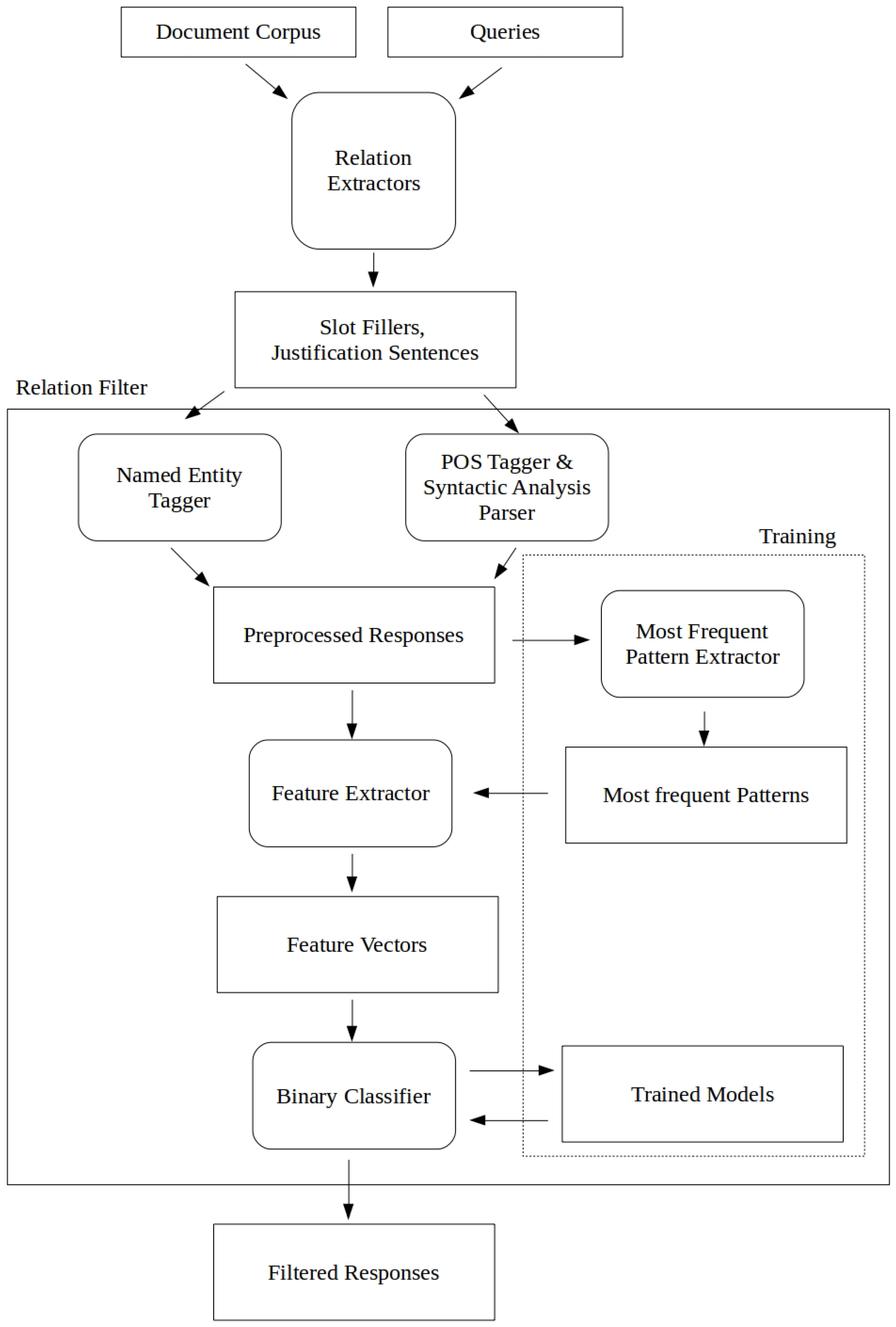
Our approach consists of using a machine learning filter trained on the combined outputs of the TAC ESF participating systems. For each relation, a binary classifier filter is appended to the end of a relation extractor, from where it eliminates responses, which it classifies as wrong. Figure 1 shows the general data flow: justification sentences from relation extractors are preprocessed and then features are extracted from these sentences for classification. This approach aims at improving the precision of any relation extractor. An increase in recall is not possible because there are not any additional responses generated by our filter. The training data is aggregated and preprocessed in the following manner. The outputs from the relation extractors, which contain a justification sentence for each response, are passed to the named-entity recognizer (NER), which gives the NE tags for each word in the justification sentences (OTHER if the word is not a named entity). The outputs from the relation extractors are also passed to the part-of-speech (POS) tagger and syntactic analysis parser, which return the POS tags as well as the syntactic dependencies tree (details in Section 3.2.3). Most frequent patterns are extracted from the raw justification sentence as well as the POS/syntactic analysis output. Sentence-level and syntactic-dependency-tree-level frequent patterns and the preprocessed responses are used for feature extraction (details in Section 3.3). The resulting feature vectors are then passed to the binary classifier for training.
3.2. Preprocessing
3.2.1. Background
As mentioned previously, the dataset is composed of responses from relation extractors to queries related to 41 pre-defined relations. Table 1 shows a complete list of the relations for the TAC KBP 2013 ESF task. There are 25 relations expected to be filled for requests of entity type person and 16 relations for requests of entity type organization [24]. Responses are assessed as either correct, if they satisfy the assessment validity criterion, and wrong otherwise. The table also shows the distribution of the complete training dataset, comprising the preprocessed responses of each relation extractor’s best run after the dataset is cleaned (details in Section 3.2.2). The amount of training data varies widely across relations, primarily because some relations expect multiple values, whereas others only expect a single value as filler, and secondly because relation extractors have more ease in generating and retaining candidates for certain relations compared to others. Another important fact to consider is the class imbalance towards the wrong class in most relations.
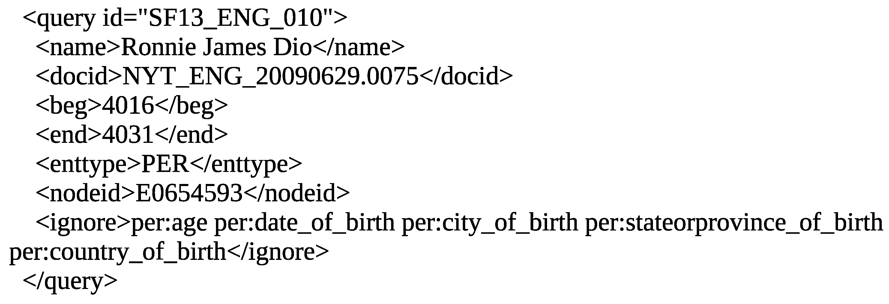
The relation extractors were provided a list of 100 queries that consisted of a named entity and a list of relations to fill [4]. Figure 2 shows an example of a query. The XML query contains the query ID, the named entity, the ID of a document in which an instance of the entity can be found, and the beginning and end character offset of this instance in the document. The query also contains the entity type (organization or person) indicating which relations have to be extracted. If the entity is already in the knowledge base, it also contains a node ID and a list of slots that must be ignored (because they are already available in the knowledge base). In response to the input queries, systems’ submissions were required to provide the following information in each individual answer: the query ID, the ID of the document that contains the answer, the name, string or value that is related to the relation specified in the query (we will call this the slot filler), the offset of the query entity in the document, the offset of the slot filler, the beginning/end character offset of the justification text, and, finally, a confidence score [4]. For a given query, slots are expected to be filled for all relations associated with the entity type (except for relations to be ignored). Some relations accept multiple answers, e.g., alternate_names, children, title, etc. Name slots are required to be filled with the name of a person, organization or geo-political entity; value slots are required to be filled by either a numerical value or a date; string slots are a “catch all” meaning that their fillers cannot be classified as names or values [24]. All answers come from the Linguistic Data Consortium (LDC) Corpus entitled “the TAC 2013 KBP Source Corpus” (catalog ID: LDC2013E45) composed of 2.1 million documents: 1 million newswire documents from Gigaword, 1 million web documents and 100,000 documents from web discussion forums [4]. Systems were also required to submit between one and five system runs for which the system configuration could vary. Each run is annotated by the LDC assessors who classify each response as correct if the slot filler and its justification are accurate and wrong otherwise. For our experiment, we used the data from the evaluation queries for the TAC KBP 2013 Slot Filler Validation (SFV) track, which are composed of the annotated ESF submissions. The complete dataset utilized for our experiment is the pool of annotated data made of each participating systems best run, i.e., the run that achieved the highest F1 score.
3.2.2. Dataset Cleaning and Partition
As mentioned, the TAC KBP English Slot Filling task only requires systems, for every output, to provide the query entity, the slot filler and justification, the ID of the document where they are found and the beginning/end character offset of the filler, the query and the justification in this document. The document ID and offsets constitute the data that is used to train and test our classifiers and are in some cases noisy, since some relation extractors provide erroneous offsets. For example, although some source documents are in HTML, some systems do not consider HTML tags in their computation of offsets. Therefore, the justification cannot be properly recovered. To ensure the cleanliness of the data, such outputs are removed from the training set. Responses containing a justification with a character length greater than 600 are removed from the dataset as well to ensure a smooth usage of the Stanford Parser. We removed HTML tags from responses in the query entity, the slot filler, or the justification. We also removed periods, question marks and exclamation marks from responses that contained such punctuations at the beginning of their justification.
For a given system, we hold out its own output from the training set and use it as test data in order to be able to compare the system’s initial performance to its performance after filtering using the official evaluation script. This means no actual data coming from the system is used in the training set. The evaluation script calculates the global recall, precision and F1 by considering only the slots for which the system submitted a response or nil, which indicates the system is confident no response can be found. We have also experimented a segmentation where 75% of slots were used for training and 25% of slots were held for the test dataset. This enables us to include a portion of the tested system’s output in the training data; however, we can only test the filter’s performance on 25% of the system’s output. We have not noticed a significant increase nor decrease in performance for the tested slots compared to the previous segmentation. We therefore make the assumption that there is no significant variability between outputs of different systems affecting the filter’s performance and proceed using the former train/test segmentation to be able to compare the systems’ performances after filtering to their original performance.
3.2.3. Linguistic Processing of Justifications
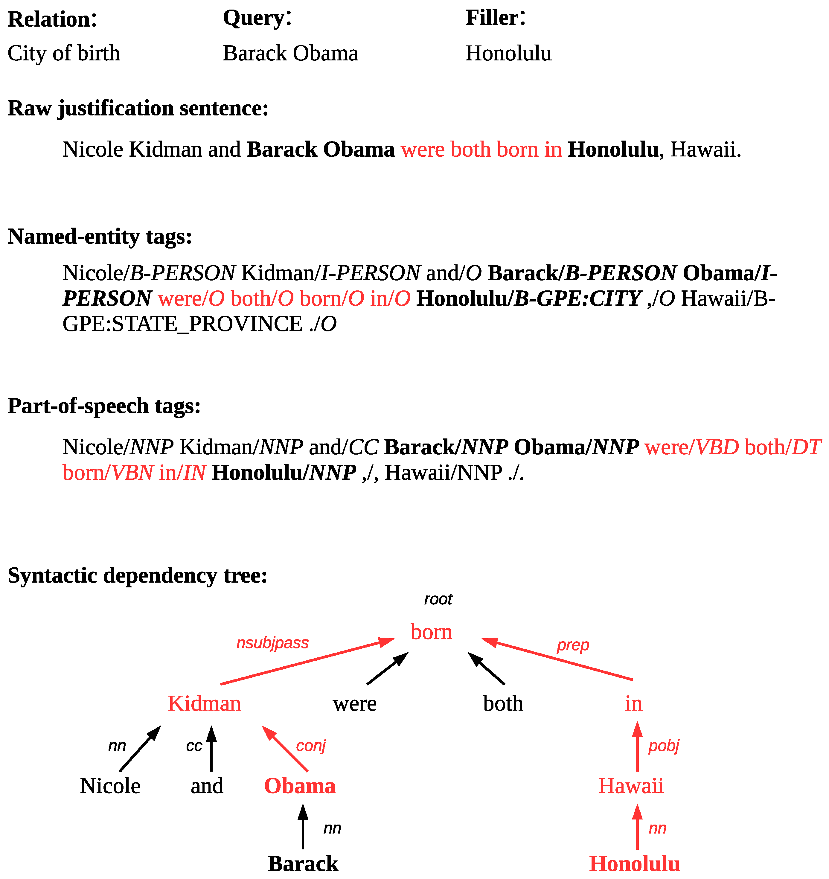
The various features require the justification to be annotated with part-of-speech tags as well as named-entity tags. The syntactic dependencies tree is also necessary for feature extraction. Systems are allowed to submit up to two sets of character offsets within the specified document to designate query entity, slot filler and justification. Therefore, since most features depend on the query entity and the slot filler’s position in the justification, we must ensure a mapping between these positions and the justification sentence. This process is necessary, especially in cases where there are multiple references to either the query entity or the slot filler in the justification or if either entity is designated by a pronoun. We used the Stanford Parser to obtain the part-of-speech annotated justification as well as the syntactic dependencies [25]. The named-entity annotations are obtained by applying sequor, a perceptron named-entity tagger [26]. Figure 3 shows an example of a justification sentence for which the named-entity tags, the part-of-speech tags and the syntactic dependency tree have been extracted.
3.2.4. Down-Sampling and Selective Filtering
In order to avoid overfitting, we do not filter relations for which the number of instances is inferior to 15 for either class (correct/wrong). Due to the lack of available examples, the following relations were omitted from the filtering process for all systems: org:date_dissolved, org:member_of, org:political_religious_affiliation, per:county_of_birth, per:religion. Data imbalance have been shown to cause classifiers to favor the majority class [27]. For most relations, there are more wrong instances than correct instances. Therefore, for each relation where the number of wrong instances is greater than two times the number of correct instances, we down-sample the subset of wrong instances to five subsets randomly sampled containing the same number of instances as the correct class subset. The usage of these five subsets will be further detailed in Section 3.4. The training dataset was rebalanced for the following relations for most systems: org:founded_by, org:members, org:parents, org:subsidairies, per:charges, per:cities_of_residence, per:countries_of_residence, per:employee_or_member_of, per:origin, per:other_family, per:parents, per:siblings, per:statesorprovinces_of_residence. Other relations were either rebalanced or eliminated for a few systems.
3.3. Features
The main goal of our approach is to experiment with various sets of features and ultimately propose a relation-independent selection of features. In this section, we present a set of generic features used in our experiment.
Our approach is based on a wide selection of generic features ranging from statistical, named-entity, lexical to syntactic features. These features are listed in Table 2.
3.3.1. Statistical Features
Our filter utilizes generic features such as sentence length (C1), the number of words of both the query entity and the slot filler (two features) (C2), and their order of appearance in the justification sentence, either query or filler first (C3). Another set of features is based on the segmentation of the sentence according to the position of the query entity and the slot filler, resulting for most sentences in three segments (before, between and after the query entity and slot filler). For each sentence segment, we capture the number of tokens (including words and punctuation) (C4). Since the training data is directly derived from relation extractors that participated in the TAC KBP English Slot Filling task, and given that the task requires every submitted response to be accompanied by a confidence score, we exploit this score as a feature (C5).
3.3.2. Named Entity Features
This subset of features captures the location of named entities in the justification relative to the query and the filler for the following types: person (N1), geo-political entity (N2) and organization (N3) [28]. Similarly to feature C4, this set of features is based on the segmentation of the sentence according to the position of the query entity and the slot filler. For each sentence segment, we capture the number of named entities of each of the specified types, resulting in three features for each entity type. For example, as shown in Figure 3, given the relation city of birth, in the following justification, “Nicole Kidman and Barack Obama were both born in Honolulu, Hawaii.”, where the query entity is Barack Obama and the slot filler is Honolulu, the sentence would be segmented in the following way: (1) Nicole Kidman and (2) were both born in (3), Hawaii. The first segment contains one entity of type person (Nicole Kidman), the second segment does not contain any named entity and the final segment contains one named entity of type geo-political entity (Hawaii).
3.3.3. Lexical (POS) Features
Our filter also relies on a subset of features that captures the ratio of part-of-speech tags in each sentence segment and in the whole sentence. The part-of-speech tags are generalized into four categories: nouns, verbs, adjectives and other (L1) [28]. If we take Figure 3, for example, the distribution of POS tags for the sentence segment before the query entity (“Nicole/noun Kidman/noun and/other”) is the following: nouns: 2/3, verbs: 0/3, adjectives: 0/3, other: 1/3. We also extracted the most frequent subsets of part-of-speech tags between both entities at the sentence level in the training dataset (L2). This is done using the Apriori algorithm after separating the instances of each relation by class (correct and wrong) [29]. We used a support of 0.15, meaning that the subset must be present in at least 15% of data related to the wanted class. The Apriori algorithm allows for retaining the desired subsets with reduced computational resources, by first identifying individual items, in this case a single POS tag, for which the support is greater than the minimum support and extending them to larger item sets by retaining only the subsets that have a support greater than the minimum support, 15% in this case. In order to ensure the specificity of the previously withheld subset, a subset is only retained if its support on the opposite class is equal to or less than 0.5 of its support on the wanted class (we will call this value specificity), which gives us a minimum specificity of 2. These parameters were determined experimentally. In order to maintain a reasonable training execution time, we have limited the number of retained subsets to 100. As long as the number of retained subsets is greater than the limit, we rerun the Apriori algorithm with a 2% support increment and a 10% specificity increment. The number of retained subsets ranges from 1 to 100 in the 41 relations. We derive boolean features that indicate the presence or absence of each subset between the query and the filler at the sentence level. A similar method is used to extract the most frequent word subsets contained in the whole sentence (bag of words) (L3). Stop words, named-entities and punctuation are excluded from potential subsets. Figure 3 shows an example of a justification sentence for which the query is Barack Obama and the filler is Honolulu. In this case, the word set is the following : {born}. The other words between the query and the filler are either named entities or stop-words and are therefore not retained. Since word subsets are more specific to responses compared to POS subsets, we used Apriori with more lenient parameters to retain the most frequent subsets in the training data: support 10%, specificity 1.5, limit of retained subsets 200, support increment 1% and specificity increment 0. Similarly, we extract POS tag bigram subsets and word bigram subsets between the query and the filler and retain the most frequent subsets using the Apriori algorithm once again (L4 and L5). We also add two additional tokens representing respectively the query and the filler to the bigram subset. In order to retain a sufficient amount of subsets, we use the following settings: support 5%, specificity 1.5, limit of retained subsets 200, support increment 1% and specificity increment 0. The word bigram subset is the following for the example shown in Figure 3: {QUERY_were, were_both, both_born, born_in, in_FILLER}. The POS bigram subset is constituted of the corresponding POS tags: {QUERY_VBD, VBD_DT, DT_VBN, VBN_IN, IN_FILLER}.
3.3.4. Syntactic features
These features are based on the syntactic dependency tree obtained by parsing the justification sentence. The distance between both entities, i.e., the query and the filler (S1), is the number of links that separate both entities in the syntactic dependency tree. The entity level difference (S2) is the difference between the level (depth) of each entity in the tree. We use a feature that indicates if one entity is the ancestor of the other (S3). We also focus on frequent subsets between the entities in the syntactic dependency tree. The subsets retained are comprised of syntactic dependencies of words present in the subtree between both entities (path in the tree between both entities) (S4). In cases where either entity is composed of more than one word, we consider only the word with the lowest level to represent the query or the filler. For example, in Figure 3, the query has two words, Barack and Obama. Since the level of Barack is 3 and the level of Obama is 2 (root level = 0), we consider only Obama as the query for the subset extraction. This is the case for every syntactic feature. We, once again, use the Apriori algorithm, with the following parameters: support 15%, specificity 2, limit of retained subsets 100, support increment 1%, specificity increment 10%, to obtain the most frequent subsets. The syntactic dependencies subset for the example in Figure 3 is: {conj, nsubjpass, prep, pobj, nn}. Another set of features derived from most frequent subsets captures the syntactic dependencies, direction and part-of-speech tag of each node in the subtree common to both entities (S5). The direction is obtained by following the path starting from the query and ending at the filler. The Apriori algorithm is used with the same parameters as the previous set of features. Each token is comprised of the syntactic dependency, the direction (↑: the next token in the path is closer to the root, ↓: the next token in the path is further from the root, -: the token is at root level) and the POS tag. The subset for the example in Figure 3 is: {(conj,↑,NNP), (nsubjpass,↑,NNP), (root,-,VBN), (prep,↓,IN), (pobj,↓,NNP), (nn,↓,NNP)}. In the same way, we extract the syntactic dependencies bigrams as well as the syntactic dependencies, direction and part-of-speech tuple bigrams within the path between the query and the filler in the syntactic dependency tree (S6 & S7). The syntactic dependency bigram subset for the example in Figure 3 is: conj_nsubjpass, nsubjpass_prep, prep_pobj, pobj_nn. The syntactic dependencies, direction and part-of-speech tuple bigrams are the following: {(conj,↑, NNP)_(nsubjpass,↑,NNP), (nsubjpass,↑,NNP)_(root,-,VBN), (root,-,VBN)_(prep,↓,IN), (prep,↓,IN)_(pobj,↓,NNP), (pobj,↓,NNP)_(nn,↓,NNP)}. We use the Apriori algorithm to retain the most frequent subsets with the same configuration as L4 and L5 feature subsets.
3.4. Classifiers
For each relation, we trained a series of classifiers from which we selected the best classifier to apply on test data, i.e., used for filtering the relation extractors’ output. Models are selected from one of the following base classifiers: RandomForest [30,31], Sequential Minimal Optimization (SMO) [32,33,34,35], NBTree [36,37], DecisionTable [38,39], J48 [40] and K* [41,42]. The evaluation is done on the training set using a 10 fold cross-validation. We retain the classifier that has the greatest F1 measure on the correct class. We selected this metric amongst others for the sole purpose that we want to limit the number of false negatives produced by the classifier. As mentioned in the previous section, the aim of the filter is to increase the relation extractors’ global precision while limiting loss on recall. A significant amount of false negatives produced by the filter would result in a great loss of recall, which would be detrimental to the relation extractors’ F1. For relations that have been rebalanced, we train these six classifiers for the five randomly sampled subsets. We retain the classifier/subset pair that has the greatest F1 measure on the correct class. We performed the experiments using Weka’s implementation of the classifiers with the default configurations and hyper-parameters [43].
4. Experiments
We performed experiments for each participating system in the TAC KBP Slot Filling task. We present results for all systems, and then we focus on Relation Factory, the best performing system [8].
4.1. Experiment Overview
From the 18 available systems, we excluded four systems because the offsets provided did not allow us to extract the queries, fillers and justifications. In fact, the following systems’ outputs are corrupted by a character offset error and were omitted in order to evaluate the filter’s performances correctly: SINDI, IIRG, CohenCMU and Compreno. The experiment is executed for each of the remaining 14 participating systems by holding out its own output from the training data. The following description indicates the procedure for one system. Once the preprocessed training data is separated by relation, the features are extracted from each response. In some cases, some features may not be extracted if they depend on the position of the query entity and the slot filler in the justification sentence (e.g., the distance between entities in the syntactic tree, the ratio of part-of-speech tags of each type between the entities at the sentence level, etc. ). In general, when this happens, it is due to the fact that one of the entities (query, slot filler) cannot be found in the justification, or because both entities cannot be found in the same sentence. The filter only processes responses in which a reference to both entities is present in the same sentence. When both entities are not found in the same sentence, most features cannot be extracted. Therefore, the response is removed from the training set. The procedure for the test data is quite similar: responses for which entities are not found in the same sentence are simply not passed through the filter and are kept by default. Cases for which the responses are rejected correspond to approximately 15% of the instances and are unevenly distributed amongst relations. For relations such as org:website, systems do not typically return complete sentences as justifications, but only return short textual segments generally containing only the filler. Specific relations such as per:alternate_names and org:alternates_names, for which justifications are not required to obtain a correct assessment are the main cause of examples being rejected from the training set.
The filtered response is evaluated using the TAC KBP 2013 English Slot Filling evaluation script version 1.4.1 (http://www.nist.gov/tac/2013/KBP/SentimentSF/tools/SFScore.java) with the strict configuration, for which the response is assessed as correct only if the answer is provided with a correct justification. As mentioned previously, from the 18 systems, we excluded four systems because their output was not processable. Our filter enables an increase in precision for every relation extractor that participated in the TAC KBP 2013 English Slot Filling task compared to its original performance. We have attempted multiple feature configurations to train our classifiers. We have achieved the greatest precision increase using a combination of statistical and lexical/POS features using bigrams as a base for the extraction of most frequent subsets (subsets composed respectively of POS and word bigrams). Table 3 shows the evaluation for participating systems before and after filtering using this feature configuration. The filter results in an average increase in precision of 11.2% and an average decrease in recall of 4.4% for the 14 systems. It allows an increase in precision for every system and an F1 increase for three systems including Relation Factory, the best performing system. In the case of Relation Factory, the precision increases from 42.5% to 63% with a 20.5% increase. The F1 is increased from 37.3% to 38.4%.
4.2. Evaluation by Relation
Table 4 shows the filter’s accuracy and F1 for both correct and wrong classes evaluated by cross-validation using 10 folds on the training data. The training data contains the output of every participating system from which Relation Factory’s output was held out. Table 5 details the performances of Relation Factory, the best system of the 2013 campaign, for each relation before and after filtering using its best feature set configuration (detailed in Section 4.3) individually for every relation. From the 33 relations out of 41 for which there was a trained classifier, the filter increases the precision as well as the F1 for 20 relations. There is an increase in precision but a decrease in F1 for nine relations. There was no change in precision or F1 for three relations. Finally, the precision along with the F1 are decreased for one relation.
We separated relations based on slot quantity, slot content, number of training instances, initial recall and initial precision. Table 6 shows the difference in recall, precision and F1 after filtering Relation Factory’s output for the different relation groups. The filter has a greater impact on list-value slots for which the precision is increased by 18.3% on average relative to 13.5% for single-value slots. List-value slots have a greater contribution on global performances since they represent 73.5% of the system’s recall, whereas single slots represent 26.5% of the system’s recall. The filter increases the precision of name and string slots by respectively 17.3% and 19.3%, whereas it increases precision of value slots by only 9.8%. Table 6 also indicates that relations with a greater number of training instances achieve a greater increase in precision on average. Initial recall has a slight influence on precision increase. However, relations with a high initial recall achieve greater F1 increase. Relations with high initial precision (≥65) achieve less precision increase than relations with a lower initial precision. Relations for which initial precision is less than 40% achieve the greatest F1 increase (2.4%).
An important point to consider is the fact that the quantity of data is unevenly distributed across relations. For relations that do not have enough data, models could suffer from over-training. Therefore, it is wiser not to apply the filter in those cases, to avoid a significant decrease in performance. In addition to that, there is a great potential for improvement for the filter, considering the small amount of labeled data available for this experiment. Obviously, with a greater amount of training data, the filter would cover a greater scope of examples and would be more flexible. Improvements that were not included in this paper suggest an optimization of the current features, especially for the selection of the most frequent subsets.
4.3. Evaluation by Feature Subset
We proceeded iteratively to measure the impact of the different features throughout the experiment. We compared the results using the full set of features to those obtained using different combinations of feature subsets presented in Section 3.3. We started by varying the feature subsets in our classifiers when filtering Relation Factory’s output. Table 7 shows the performance achieved by Relation Factory after filtering using different feature configurations. For the Lexical/POS and Syntactic feature subsets, we specified if the most frequent subset based features were bigram subsets. Cases for which nothing is specified indicate that the most frequent subset based features were unigram subsets. For the Lexical/POS feature subset, we also specify if only word or POS patterns were used, and, for the Syntactic feature subset, we specify if only syntactic or multilevel subsets were used. In addition to the different feature subsets applied to our filter, the table also shows as a baseline the evaluation obtained by Relation Factory’s highest F1 run (to which the filter is applied). The run only uses its main components, which are the support vector machine (SVM) classifier, the distant supervision patterns, the hand-written patterns and the alternate name expansion modules [8]. We also compare our results to Relation Factory’s highest precision run, which uses syntactic patterns instead of the SVM classifier [8]. We first measured the impact of each feature subset used in combination with the statistical features subset. When using bigrams instead of unigrams for lexical/POS features, we obtain the best results when combined with statistical features. The precision is 0.63, and the F1 is 0.384, which is a 12.1% precision increase and a 4.1% F1 increase compared to Relation Factory’s precision run (baseline 2). It is also a 20.5% precision increase and a 1.1% F1 increase compared to Relation Factory’s F1 run (baseline 1).
To evaluate the statistical significance of our results (recall loss and precision gain), we used the chi-square test [44]. Relation Factory submitted a total of 1145 responses on which the filter was applied. Considering that the precision increases to 0.63 from 0.425 (baseline 1) and from 0.509 (baseline 2) we obtain p-values of, respectively, 5.6 × 10 and 5.0 × 10. Since the post-filtering subset is not independent from the pre-filtering subset in the case of baseline 1, we created two independent data subsets. We split Relation Factory’s output into two randomly sampled subsets: we calculated the initial precision on the first subset and applied the filter to the second subset on which we then calculated the precision. We repeated the process 100 times to obtain an average p-value. We can therefore reject the null hypothesis (p < 0.1) and consider those results as statistically significant. Considering the precision difference between the best feature subset (Statistical + Lexical/POS (bigrams)) performance (0.63) and the other subsets for which the precision ranges from 0.574 to 0.623, we obtain p-values greater than 0.1. Thus, we cannot state that the Statistical + Lexical/POS (bigrams) allows a significant precision increase over the other feature subsets. Since the different subsets are not independent, we once again split Relation Factory’s output into two randomly sampled subsets. We then applied the filter using the Statistical + Lexical/POS (bigrams) feature configuration on one subset and alternatively applied the filter using every other feature configuration on the other subset. Initially, Relation Factory has submitted 487 correct responses from 1468 responses contained in the gold standard obtaining a recall of 0.332 (baseline 1). Considering that the recall decreases from 0.332 to 0.276 (Statistical + Lexical/POS (bigrams)), we obtain a p-value of 0.0287 indicating the recall decrease is statistically significant.
Based on the results obtained by filtering Relation Factory’s output, for the seven feature subsets that allow an increase in F1 for Relation Factory, we have tested our filter for the other systems as well. Table 8 shows the average performances for the 14 systems that were tested. The greatest average precision increase was obtained using the Statistical + Lexical/POS (bigrams) feature subset, which is the same feature subset providing the greatest precision and F1 increase for Relation Factory. However, we assume there is no statistical significance between the precision difference obtained using the different subsets.
4.4. Filtering All System Runs
As mentioned previously, relation extractors were required to submit between one to five runs. This provided the opportunity for the teams to test their different system configurations. The systems that submitted multiple runs generally have precision-oriented and recall-oriented configurations. Table 9 shows the evaluation before and after filtering for all system runs. Precision is increased for 43 out of 44 runs and F1 is increased for 11 out of 44 runs (25%). The filter has increased the F1 for at least one run for 5 out of 14 systems. When applied to Relation Factory’s highest Recall run, the precision is increased by 20.9% and the F1 is increased by 3%. This post-filtering F1 of 39.4% is also a 2.1% increase relative to Relation Factory’s highest F1 run. Table 10 shows the average results for respectively every system’s F1-tuned, precision-tuned and recall-tuned run. Our filter consistently increases the original system precision by an average of at least 10% for any system configuration. However, the filter decreases the systems’ F1 by an average of 2.4% for precision-tuned runs, 1.8% for F1-tuned runs and 1.3% for recall-tuned runs.
We have also compared our results with those obtained by filtering Relation Factory’s output using a confidence score threshold heuristic only (heuristic filter). These results are shown in Table 11. By filtering Relation Factory’s output using only the confidence score, there is no confidence score threshold that achieves a higher precision or F1 than those obtained using our filter. This confirms that our filter achieves a much greater precision than tuning an individual system by increasing the threshold on the confidence score which also severely hinders the recall. To evaluate the statistical significance of our results (precision gain), we once again used the chi-square test [44]. Column p-value (p/baseline) indicates the p-value of the precision increase using the heuristic filter compared to the baseline. We measured this value using the same process as described in Section 4.3. The precision increase is statistically significant for a confidence score threshold of 0.4 to 1.0. Column p-value (p/filter) indicates the p-value of the precision difference between our filter and the heuristic filter for different confidence score values. The precision difference is statistically significant for a confidence score threshold of 0.1 to 0.7. However, using a heuristic filter based on a confidence score threshold above 0.7 hinders the recall much more (>10 percentage points) than our filter. This recall difference is statistically significant as well.
As mentioned in previous sections, our approach aims mainly at increasing the relation extractor’s precision. Our filter is appended to the end of the relation extractor’s pipeline, thus allowing the filter to be tested and operated on any system. This approach, however, imposes an upper bound on recall, which is the recall of the system before filtering. As shown in Table 9, post-filtering performances are optimal for recall-oriented system configurations. In order to increase the relation extractor’s recall, the filter would have to be directly inserted inside the pipeline after the candidate generation stage. Our modular approach gives us the flexibility to operate upstream or downstream of the candidate validation stage, whereas typical ensemble learning methods can only be applied downstream. This approach would require further specificity in order to adapt to each individual system. The system’s original candidate validation module could be improved by taking into account our filter’s confidence score for each response. An upstream integration could be a promising avenue to explore given that the filter performs best on high-recall outputs.
In line with the same idea, since the relation extractor’s recall can only decrease after filtering downstream, it is imperative to limit the loss of recall. The loss of recall is caused by the filter’s rejecting correct instances provided by the relation extractor. This case is recognized as a False Negative. Therefore, the selection of a convenient classifier for filtering is based upon the metric that is correlated with the quantity of false negatives. A high recall on the correct class indicates that a low rate of false negatives are generated at training time by the filter (Recall = TP/(TP + FN)). However, we also want to limit the number of False Positives, which in this case is a wrong response retained by the filter. A high precision on the correct class indicates a low rate of false positives (Precision = TP/(TP + FP)). Therefore, we use the F1, which is a harmonic mean of both recall and precision, to determine the base classifier. Classifiers that exhibit a high F1 on the correct class at training time and are trained on a sufficient amount of training data usually perform well on the test data. To measure the impact of our algorithm selection, we tested our filter consistently using alternately each algorithm for all relations. Results of performances on Relation Factory’s output are shown in Table 12. From the six machine learning algorithms, Random Forest provides the best performances with a 62.2% precision and a 38% F1 compared to a 63% precision and a 38.4% F1 when using our proposed algorithm selection method (Statistical and Lexical/POS (bigrams) features). For applications using limited resources, a filter using Random Forest as the default classifier could be considered without expecting a significant decrease in performances.
5. Discussion
One of the main objectives of this research was to determine the most important features for the filtering step (RQ1). Our results show that the greatest performances were achieved using a combination of statistical and POS/lexical features. Our results also show that the most frequent subsets are more informative when considering bigrams over unigrams. Bigram subsets implicitly capture the token sequence, whereas unigram subsets do not. Another objective of our research was to evaluate whether a method based on a generic set of features could lead to an increase in precision without a major setback in recall (RQ2). Since our approach imposes an upper bound on recall, which is the recall of the system before filtering, post-filtering performances are optimal for recall-oriented system configurations. Finally, we wanted to determine whether some relations were more sensitive to our filter (RQ3). The filter has a greater impact on list-value slots, which generally have a greater number of training instances. Initial recall has a slight influence on precision increase. However, relations with a high initial recall achieve greater F1 increase. The features used for training are mostly generic and could be utilized for any pre-defined relation. However, classification is more successful when there is a sufficient amount of training data that is balanced between the correct and wrong class.
An interesting path to explore in the future is feature selection. Currently, most features are generated by capturing most frequent patterns at different levels using the Apriori algorithm. The selection criteria allow us to retain patterns for which the number of occurrences in the subset of the specified class is above a certain threshold and for which the number of occurrences in the subset of the complementary class is below a certain threshold. However, for certain relations such as per:title for instance, there is a wide array of patterns that exist to represent the relation. Therefore, in order to ensure an optimal coverage, an option would be to be more lenient on Apriori selection parameters and instead use feature selection algorithms such as information gain [45] to empirically discover the most significant features for each relation.
The relation would have an even greater impact with more training data. The simplest way to increase the amount of training would be to append to the current training dataset the responses for the systems having participated in the TAC KBP English Slot Filling track in the subsequent years when they are available. However, the data would still be unevenly distributed across relations and the observable imbalance towards the wrong class would persist and we would lose data by down-sampling the dataset. We could use existing methods for up-sampling the minority class instead. One way to do so could be by using the Synthetic Minority Over-sampling Technique (SMOTE) method [46]. This method consists in creating “synthetic” examples rather than over-sampling by duplicating existing examples. This is done by creating a feature vector between a randomly selected minority class example and its nearest neighbor and adding this vector multiplied by a random number between 0 and 1 to the original selected minority class example. Finally, making use of distant supervision to increase the amount of training data would be an avenue worth considering.
6. Conclusion
This paper presented a method to increase the precision of relation extractors. This generic method consists of appending a machine learning-based filter to the relation extractor’s pipeline in order to increase its performance. The filter is based on a wide scope of features, including statistical, lexical/POS, named entity and syntactic features. We showed that precision could be increased for all the participating systems in the TAC KBP 2013 ESF track. Overall, the filter enabled a 20.5% precision increase and a 1.1% F1 increase for the best performing system from the 2013 slot filling track when applied to the F1-tuned run. The filter also led to a 14.9% precision increase and a 3% F1 increase for the best performing system when applied to the recall-tuned run. In fact, our filter performs best on high recall runs. Finally, the filter obtained a 2.1% F1 increase compared to the original F1-tuned run, the best global performance in the TAC KBP 2013 ESF track.
Author Contributions
K.L.D.C., A.Z., M.G. and L.J.-L. conceived the approach and methodology. K.L.D.C. implemented the approach and conducted the experiments on the Slot Filling Task. The supervision of this project and Masters thesis was done by M.G., A.Z. and L.J.-L.
Funding
This research was partially funded by the Fonds de recherche du Québec—Nature et technologies (FRQNT) - Industrial Innovation Scholarships Program.
Conflicts of Interest
The authors declare no conflict of interest.
References
- Singhal, A. Introducing the Knowledge Graph: Things, Not Strings. In Official Google Blog; Google Blog: Mountain View, CA, USA, 2012. [Google Scholar]
- Bizer, C.; Lehmann, J.; Kobilarov, G.; Auer, S.; Becker, C.; Cyganiak, R.; Hellmann, S. DBpedia—A Crystallization Point for the Web of Data. Web Semant. Sci. Serv. Agents World Wide Web 2009, 7, 154–165. [Google Scholar] [CrossRef]
- Bizer, C.; Heath, T.; Berners-Lee, T. Linked Data—The Story so Far. Int. J. Semant. Web Inf. Syst. 2009, 5, 205–227. [Google Scholar] [CrossRef]
- Surdeanu, M. Overview of the TAC2013 Knowledge Base Population Evaluation: English Slot Filling and Temporal Slot Filling. In Proceedings of the Sixth Text Analysis Conference (TAC 2013), Gaithersburg, MA, USA, 18–19 November 2013. [Google Scholar]
- Surdeanu, M.; Ji, H. Overview of the English Slot Filling Track at the TAC2014 Knowledge Base Population Evaluation. In Proceedings of the Text Analysis Conference Knowledge Base Population (KBP) 2014, Gaithersburg, MA, USA, 17–18 November 2014. [Google Scholar]
- Ellis, J. TAC KBP Reference Knowledge Base LDC2009E58; Linguistic Data Consortium: Philadelphia, PA, USA, 2013. [Google Scholar]
- Angeli, G.; Gupta, S.; Jose, M.; Manning, C.D.; Ré, C.; Tibshirani, J.; Wu, J.Y.; Wu, S.; Zhang, C. Stanford’s 2014 Slot Filling Systems. In Proceedings of the Text Analysis Conference Knowledge Base Population (KBP) 2014, Gaithersburg, MA, USA, 17–18 November 2014. [Google Scholar]
- Roth, B.; Barth, T.; Wiegand, M.; Singh, M.; Klakow, D. Effective Slot Filling Based on Shallow Distant Supervision Methods. arXiv, 2014; arXiv:1401.1158. [Google Scholar]
- Mintz, M.; Bills, S.; Snow, R.; Jurafsky, D. Distant Supervision for Relation Extraction without Labeled Data. In Proceedings of the Joint Conference of the 47th Annual Meeting of the ACL and the 4th International Joint Conference on Natural Language Processing of the AFNLP, Suntec, Singapore, 2–7 August 2009; Association for Computational Linguistics: Stroudsburg, PA, USA, 2009; Volume 2, pp. 1003–1011. [Google Scholar]
- Jiang, J. Domain Adaptation in Natural Language Processing; ProQuest: Ann Arbor, MI, USA, 2008. [Google Scholar]
- Fader, A.; Soderland, S.; Etzioni, O. Identifying Relations for Open Information Extraction. In Proceedings of the Conference on Empirical Methods in Natural Language Processing, Edinburgh, UK, 27–31 July 2011; Association for Computational Linguistics: Stroudsburg, PA, USA, 2011; pp. 1535–1545. [Google Scholar]
- Nguyen, T.H.; He, Y.; Pershina, M.; Li, X.; Grishman, R. New York University 2014 Knowledge Base Population Systems. In Proceedings of the Text Analysis Conference Knowledge Base Population (KBP) 2014, Gaithersburg, MA, USA, 17–18 November 2014. [Google Scholar]
- Brin, S. Extracting Patterns and Relations from the World Wide Web. In The World Wide Web and Databases; Springer: Berlin/Heidelberg, Germany, 1999; pp. 172–183. [Google Scholar]
- Agichtein, E.; Gravano, L. Snowball: Extracting Relations from Large Plain-text Collections. In Proceedings of the Fifth ACM Conference on Digital Libraries, San Antonio, TX, USA, 2–7 June 2000; ACM: New York, NY, USA, 2000; pp. 85–94. [Google Scholar]
- Li, Y.; Zhang, Y.; Doyu Li, X.T.; Wang, J.; Zuo, N.; Wang, Y.; Xu, W.; Chen, G.; Guo, J. PRIS at Knowledge Base Population 2013. In Proceedings of the Sixth Text Analysis Conference (TAC 2013), Gaithersburg, MA, USA, 18–19 November 2013. [Google Scholar]
- Roth, B.; Chrupala, G.; Wiegand, M.; Singh, M.; Klakow, D. Generalizing from Freebase and Patterns Using Distant Supervision for Slot Filling. In Proceedings of the Fifth Text Analysis Conference (TAC 2012), Gaithersburg, MA, USA, 5–6 November 2012. [Google Scholar]
- Chen, Z.; Tamang, S.; Lee, A.; Li, X.; Passantino, M.; Ji, H. Top-Down and Bottom-Up: A Combined Approach to Slot Filling. In Proceedings of the 6th Asia Information Retrieval Societies Conference, AIRS 2010, Taipei, Taiwan, 1–3 December 2010; Springer: Berlin/Heidelberg, Germany, 2010; pp. 300–309. [Google Scholar]
- Schlaefer, N.; Ko, J.; Betteridge, J.; Pathak, M.A.; Nyberg, E.; Sautter, G. Semantic Extensions of the Ephyra QA System for TREC 2007. In Proceedings of the Sixteenth Text REtrieval Conference, TREC 2007, Gaithersburg, MA, USA, 5–9 November 2007; Volume 1, p. 2. [Google Scholar]
- Moro, A.; Li, H.; Krause, S.; Xu, F.; Navigli, R.; Uszkoreit, H. Semantic Rule Filtering for Web-scale Relation Extraction. In The Semantic Web–ISWC 2013; Springer: Berlin/Heidelberg, Germany, 2013; pp. 347–362. [Google Scholar]
- Angeli, G.; Tibshirani, J.; Wu, J.Y.; Manning, C.D. Combining Distant and Partial Supervision for Relation Extraction. In Proceedings of the 2014 Conference on Empirical Methods in Natural Language Processing (EMNLP), Doha, Qatar, 25–29 October 2014. [Google Scholar]
- Surdeanu, M. Slot Filler Validation at TAC 2014 Task Guidelines; TAC: Geelong, Australia, 2014. [Google Scholar]
- Wang, I.J.; Liu, E.; Costello, C.; Piatko, C. JHUAPL TAC-KBP2013 Slot Filler Validation System. In Proceedings of the Sixth Text Analysis Conference (TAC 2013), Gaithersburg, MA, USA, 18–19 November 2013; Volume 24. [Google Scholar]
- Rajani, N.F.; Viswanathan, V.; Bentor, Y.; Mooney, R.J. Stacked Ensembles of Information Extractors for Knowledge-Base Population. In Proceedings of the 53rd Annual Meeting of the Association for Computational Linguistics (ACL-15), Beijing, China, 26–31 July 2015; Volume 1, pp. 177–187. [Google Scholar]
- Ellis, J. TAC KBP 2013 Slot Descriptions; TAC: Geelong, Australia, 2013. [Google Scholar]
- De Marneffe, M.C.; MacCartney, B.; Manning, C.D. Generating Typed Dependency Parses from Phrase Structure Parses. In Proceedings of the 2006 LREC, Genoa, Italy, 28 May 2006; Volume 6, pp. 449–454. [Google Scholar]
- Chrupała, G.; Klakow, D. A Named Entity Labeler for German: Exploiting Wikipedia and Distributional Clusters. In Proceedings of the Conference on International Language Resources and Evaluation (LREC), Valletta, Malta, 17–23 May 2010; pp. 552–556. [Google Scholar]
- Chawla, N.V. Data Mining for Imbalanced Datasets: An Overview. In Data Mining and Knowledge Discovery Handbook; Springer: Berlin/Heidelberg, Germany, 2005; pp. 853–867. [Google Scholar]
- Voskarides, N.; Meij, E.; Tsagkias, M.; de Rijke, M.; Weerkamp, W. Learning to Explain Entity Relationships in Knowledge Graphs. In Proceedings of the 53rd Annual Meeting of the Association for Computational Linguistics and the 7th International Joint Conference on Natural Language Processing, Beijing, China, 26–31 July 2015. [Google Scholar]
- Agrawal, R.; Srikant, R. Fast Algorithms for Mining Association Rules. In Proceedings of the 20th International Conference on Very Large Data Bases; Morgan Kaufmann Publishers, Inc.: Burlington, MA, USA, 1994; Volume 1215, pp. 487–499. [Google Scholar]
- Breiman, L. Random forests. Mach. Learn. 2001, 45, 5–32. [Google Scholar] [CrossRef]
- Breiman, L. Bagging Predictors. Mach. Learn. 1996, 24, 123–140. [Google Scholar] [CrossRef]
- Vapnik, V.N.; Kotz, S. Estimation of Dependences Based on Empirical Data; Springer: New York, NY, USA, 1982; Volume 40. [Google Scholar]
- Boser, B.E.; Guyon, I.M.; Vapnik, V.N. A Training Algorithm for Optimal Margin Classifiers. In Proceedings of the Fifth Annual Workshop on Computational Learning Theory, Pittsburgh, PA, USA, 27–29 July 1992; ACM: New York, NY, USA, 1992; pp. 144–152. [Google Scholar]
- Burges, C.J. A Tutorial on Support Vector Machines for Pattern Recognition. Data Min. Knowl. Discov. 1998, 2, 121–167. [Google Scholar] [CrossRef]
- Platt, J. Sequential Minimal Optimization: A Fast Algorithm for Training Support Vector Machines; Technical Report MSR-TR-98-14; Microsoft Research: Redmond, WA, USA, 1998. [Google Scholar]
- Kohavi, R. Scaling Up the Accuracy of Naive-Bayes Classifiers: A Decision-Tree Hybrid. In Proceedings of the Second International Conference on Knoledge Discovery and Data Mining, Portland, OR, USA, 2–4 August 1996; pp. 202–207. [Google Scholar]
- John, G.H.; Langley, P. Estimating Continuous Distributions in Bayesian Classifiers. In Proceedings of the Eleventh Conference on Uncertainty in Artificial Intelligence, Morgan Kaufmann, Montreal, QC, Canada, 18–20 August 1995; pp. 338–345. [Google Scholar]
- Kohavi, R. The Power of Decision Tables. In Machine Learning: ECML-95; Springer: Berlin/Heidelberg, Germany, 1995; pp. 174–189. [Google Scholar]
- Russell, S.; Norvig, P.; Intelligence, A. A Modern Approach; Artificial Intelligence; Prentice Hall: Egnlewood Cliffs, NJ, USA, 1995; Volume 25, p. 27. [Google Scholar]
- Quinlan, J.R. C4. 5: Programs for Machine Learning; Elsevier: New York, NY, USA, 2014. [Google Scholar]
- Cleary, J.G.; Trigg, L.E. K*: An Instance-based Learner Using an Entropic Distance Measure. In Proceedings of the 12th International Conference on Machine Learning, Tahoe City, CA, USA, 9–12 July 2016; pp. 108–114. [Google Scholar]
- Sharma, T.C.; Jain, M. WEKA Approach for Comparative Study of Classification Algorithm. Int. J. Adv. Res. Comput. Commun. Eng. 2013, 2, 1925–1931. [Google Scholar]
- Hall, M.; Frank, E.; Holmes, G.; Pfahringer, B.; Reutemann, P.; Witten, I.H. The WEKA Data Mining Software: An Update. ACM SIGKDD Explor. Newsl. 2009, 11, 10–18. [Google Scholar] [CrossRef]
- Mantel, N. Chi-square tests with one degree of freedom; extensions of the Mantel-Haenszel procedure. J. Am. Stat. Assoc. 1963, 58, 690–700. [Google Scholar]
- Yang, Y.; Pedersen, J.O. A Comparative Study on Feature Selection in Text Categorization. In Proceedings of the Fourteenth International Conference on Machine Learning (ICML 1997), Nashville, TN, USA, 8–12 July 1997; Volume 97, pp. 412–420. [Google Scholar]
- Chawla, N.V.; Bowyer, K.W.; Hall, L.O.; Kegelmeyer, W.P. SMOTE: Synthetic Minority Over-sampling Technique. J. Artif. Intell. Res. 2002, 16, 321–357. [Google Scholar]
Figure 1.
Pipeline describing our approach.

Figure 2.
TAC ESF query example [4].
Figure 2.
TAC ESF query example [4].

Figure 3.
Example of NE tags, POS tags and syntactic dependency tree for a justification sentence.


Table 1.
List of 41 pre-defined relations in TAC KBP 2013 English Slot Filling track and their categorization [24].
Table 1.
List of 41 pre-defined relations in TAC KBP 2013 English Slot Filling track and their categorization [24].
| Type | Relation | Content | Quantity | #Correct | #Wrong | Total |
|---|---|---|---|---|---|---|
| ORG | org:alternate_names | Name | List | 100 | 157 | 257 |
| ORG | org:city_of_headquarters | Name | Single | 62 | 118 | 180 |
| ORG | org:country_of_headquarters | Name | Single | 73 | 114 | 187 |
| ORG | org:date_dissolved | Value | Single | 0 | 15 | 15 |
| ORG | org:date_founded | Value | List | 36 | 48 | 84 |
| ORG | org:founded_by | Name | List | 49 | 127 | 176 |
| ORG | org:member_of | Name | List | 5 | 195 | 200 |
| ORG | org:members | Name | List | 49 | 195 | 244 |
| ORG | org:number_of_employees_members | Value | Single | 19 | 28 | 47 |
| ORG | org:parents | Name | List | 34 | 270 | 304 |
| ORG | org:political_religious_affiliation | Name | List | 1 | 39 | 40 |
| ORG | org:shareholders | Name | List | 15 | 255 | 270 |
| ORG | org:stateorprovince_of_headquarters | Name | Single | 47 | 76 | 123 |
| ORG | org:subsidiaries | Name | List | 46 | 259 | 305 |
| ORG | org:top_members_employees | Name | List | 392 | 612 | 1004 |
| ORG | org:website | String | Single | 79 | 17 | 96 |
| PER | per:age | Value | Single | 226 | 22 | 248 |
| PER | per:alternate_names | Name | List | 58 | 114 | 172 |
| PER | per:cause_of_death | String | Single | 127 | 110 | 237 |
| PER | per:charges | String | List | 58 | 149 | 207 |
| PER | per:children | Name | List | 169 | 202 | 371 |
| PER | per:cities_of_residence | Name | List | 71 | 356 | 427 |
| PER | per:city_of_birth | Name | Single | 44 | 56 | 100 |
| PER | per:city_of_death | Name | Single | 105 | 97 | 202 |
| PER | per:countries_of_residence | Name | List | 77 | 164 | 241 |
| PER | per:country_of_birth | Name | Single | 11 | 23 | 34 |
| PER | per:country_of_death | Name | Single | 26 | 50 | 76 |
| PER | per:date_of_birth | Value | Single | 63 | 22 | 85 |
| PER | per:date_of_death | Value | Single | 123 | 124 | 247 |
| PER | per:employee_or_member_of | Name | List | 257 | 554 | 811 |
| PER | per:origin | Name | List | 120 | 320 | 440 |
| PER | per:other_family | Name | List | 19 | 184 | 203 |
| PER | per:parents | Name | List | 80 | 167 | 247 |
| PER | per:religion | String | Single | 9 | 44 | 53 |
| PER | per:schools_attended | Name | List | 78 | 93 | 171 |
| PER | per:siblings | Name | List | 43 | 154 | 197 |
| PER | per:spouse | Name | List | 169 | 266 | 435 |
| PER | per:stateorprovince_of_birth | Name | Single | 27 | 48 | 75 |
| PER | per:stateorprovince_of_death | Name | Single | 57 | 62 | 119 |
| PER | per:statesorprovinces_of_residence | Name | List | 50 | 176 | 226 |
| PER | per:title | String | List | 888 | 1277 | 2165 |
| Total | 3962 | 7359 | 11321 |
Content: filler type (Name, Value or String), Quantity: number of fillers expected for the relation (Single or List), #Correct: number of correct responses, #Wrong: number of wrong responses, Total: number of responses.
Table 2.
Full set of generic features used for filtering.
| ID | Name | Description |
|---|---|---|
| Statistical features | ||
| C1 | Sentence length | Number of tokens in sentence |
| C2 | Answer/query length | Number of tokens within answer and query references |
| C3 | Entity order | Order of appearance of query and answer references |
| C4 | #tokens left/between/right | Number of tokens left/right or between entities in the sentence |
| C5 | Confidence score | Score given by the relation extractor [4] |
| Named-entity features | ||
| N1 | #person left/between/right | Number of person left/right or between entities in the sentence [28] |
| N2 | #gpe left/between/right | Number of Geo-political entities left/right or between entities in the sentence [28] |
| N3 | #orgs left/between/right | Number of organizations left/right or between entities in the sentence [28] |
| Lexical (POS) features | ||
| L1 | POS fractions left/between /right/sentence | Fraction of nouns, verbs, adjectives and others left/right/between answer and query references or in the whole sentence [9] |
| L2 | POS subsets | Most frequent subsets of POS tags between query and answer references in the sentence. (boolean feature indicating the presence of the subset) |
| L3 | Word subsets | Most frequent subsets of word (excluding stop-words and named entities) in the sentence. (boolean feature indicating the presence of the subset) |
| L4 | POS bigram subsets | Most frequent subsets of POS tag bigrams (excluding stop-words) between query and answer references in the sentence. (boolean feature indicating the presence of the subset) |
| L5 | Word bigram subsets | Most frequent subsets of word bigrams between query and answer references in the sentence. (boolean feature indicating the presence of the subset) |
| Syntactic features | ||
| S1 | Distance between entities | Distance between entities at the syntactic dependency tree level |
| S2 | Entity level difference | Level difference within syntactic dependency tree between query and answer references |
| S3 | Ancestors | One entity is ancestor of the other at the syntactic dependency tree level |
| S4 | Syntactic dependencies subsets | Most frequent subsets of syntactic dependencies between query and answer references at the syntactic dependency tree level (boolean feature indicating the presence of the subset) |
| S5 | Multilevel subsets | Most frequent subsets, where each token is composed of a POS tag, syntactic dependency and direction, between query and answer references at the syntactic dependency tree level (boolean feature indicating the presence of the subset) |
| S6 | Syntactic dependencies bigram subsets | Most frequent subsets of syntactic dependencies bigram between query and answer references at the syntactic dependency tree level (boolean feature indicating the presence of the subset) |
| S7 | Multilevel bigram subsets | Most frequent subsets, where each token is composed of a POS tag, syntactic dependency and direction bigram, between query and answer references at the syntactic dependency tree level (boolean feature indicating the presence of the subset) |
Table 3.
Global Evaluation using the TAC KBP 2013 Slot Filling scorer on the test dataset for all systems before and after filtering.
Table 3.
Global Evaluation using the TAC KBP 2013 Slot Filling scorer on the test dataset for all systems before and after filtering.
| System ID | Pre-Filtering | Post-Filtering | ||||
|---|---|---|---|---|---|---|
| Recall | Precision | F1 | Recall | Precision | F1 | |
| Uwashington | 0.103 | 0.634 | 0.177 | 0.079 | 0.725 | 0.143 |
| BIT | 0.232 | 0.511 | 0.319 | 0.185 | 0.668 | 0.290 |
| CMUML | 0.107 | 0.323 | 0.161 | 0.082 | 0.553 | 0.142 |
| lsv (Relation Factory) | 0.332 | 0.425 | 0.373 | 0.276 | 0.630 | 0.384 |
| TALP_UPC | 0.057 | 0.131 | 0.080 | 0.048 | 0.262 | 0.082 |
| NYU | 0.168 | 0.538 | 0.256 | 0.139 | 0.620 | 0.227 |
| PRIS2013 | 0.276 | 0.389 | 0.323 | 0.211 | 0.535 | 0.303 |
| Stanford | 0.279 | 0.357 | 0.314 | 0.208 | 0.491 | 0.293 |
| UNED | 0.093 | 0.176 | 0.122 | 0.061 | 0.249 | 0.098 |
| Umass_IESL | 0.185 | 0.109 | 0.137 | 0.153 | 0.159 | 0.156 |
| SAFT_Kres | 0.150 | 0.157 | 0.153 | 0.095 | 0.167 | 0.122 |
| CUNY_BLENDER | 0.290 | 0.407 | 0.339 | 0.221 | 0.519 | 0.310 |
| utaustin | 0.081 | 0.252 | 0.123 | 0.050 | 0.310 | 0.087 |
| ARPANI | 0.275 | 0.504 | 0.355 | 0.215 | 0.600 | 0.316 |
| Average | 0.188 | 0.351 | 0.231 | 0.144 | 0.463 | 0.211 |
Filtering has increased F1 for systems shown in bold .
Table 4.
Classifier performances on train set for Relation Factory by cross-validation (10-folds).
| Relation | Algorithm | Accuracy (%) | F1 (Correct) | F1 (Wrong) |
|---|---|---|---|---|
| org:alternate_names | NBTree | 94.7368 | 0.933 | 0.957 |
| org:city_of_headquarters | RandomForest | 74.7368 | 0.755 | 0.739 |
| org:country_of_headquarters | NBTree | 78.6207 | 0.739 | 0.819 |
| org:date_founded | NBTree | 77.4648 | 0.704 | 0.818 |
| org:founded_by | RandomForest | 92.9412 | 0.936 | 0.921 |
| org:members | SMO | 90 | 0.879 | 0.915 |
| org:number_of_employees_members | SMO | 84.375 | 0.828 | 0.857 |
| org:parents | SMO | 80.7692 | 0.808 | 0.808 |
| org:shareholders | SMO | 68.9655 | 0.69 | 0.69 |
| org:stateorprovince_of_headquarters | RandomForest | 81.25 | 0.747 | 0.851 |
| org:subsidiaries | SMO | 86.3636 | 0.847 | 0.877 |
| org:top_members_employees | RandomForest | 76.799 | 0.698 | 0.812 |
| per:alternate_names | SMO | 92.4528 | 0.917 | 0.931 |
| per:cause_of_death | J48 | 84.2932 | 0.84 | 0.845 |
| per:charges | SMO | 73.7864 | 0.743 | 0.733 |
| per:children | RandomForest | 82.6087 | 0.797 | 0.848 |
| per:cities_of_residence | SMO | 75.8929 | 0.765 | 0.752 |
| per:city_of_birth | SMO | 77.0115 | 0.744 | 0.792 |
| per:city_of_death | J48 | 81.6092 | 0.814 | 0.818 |
| per:countries_of_residence | SMO | 73.1343 | 0.746 | 0.714 |
| per:country_of_death | SMO | 82.2222 | 0.818 | 0.826 |
| per:date_of_birth | J48 | 84 | 0.895 | 0.667 |
| per:date_of_death | NBTree | 63.8498 | 0.703 | 0.539 |
| per:employee_or_member_of | NBTree | 66.4269 | 0.689 | 0.635 |
| per:origin | RandomForest | 79.1045 | 0.806 | 0.774 |
| per:other_family | J48 | 87.5 | 0.846 | 0.895 |
| per:parents | J48 | 91.8033 | 0.918 | 0.918 |
| per:schools_attended | RandomForest | 79.1367 | 0.785 | 0.797 |
| per:siblings | RandomForest | 86.9565 | 0.877 | 0.862 |
| per:spouse | RandomForest | 79.2105 | 0.727 | 0.832 |
| per:stateorprovince_of_birth | J48 | 84.058 | 0.766 | 0.879 |
| per:stateorprovince_of_death | SMO | 83.8095 | 0.825 | 0.85 |
| per:statesorprovinces_of_residence | SMO | 77.5281 | 0.773 | 0.778 |
| per:title | RandomForest | 70.96 | 0.644 | 0.755 |
Table 5.
Evaluation for Relation Factory using the TAC KBP 2013 Slot Filling scorer on the test dataset before and after filtering for each relation.
Table 5.
Evaluation for Relation Factory using the TAC KBP 2013 Slot Filling scorer on the test dataset before and after filtering for each relation.
| Relation | Pre-Filtering | Post-Filtering | ||||
|---|---|---|---|---|---|---|
| Instances | Precision | F1 | Precision | F1 | Classifier | |
| org:country_of_headquarters | 30 | 0.267 | 0.250 | 0.636 | 0.311 | NBTree |
| org:date_founded | 7 | 0.714 | 0.500 | 1.000 | 0.556 | NBTree |
| org:number_of_employees_members | 11 | 0.273 | 0.273 | 0.375 | 0.316 | SMO |
| org:parents | 16 | 0.25 | 0.276 | 0.364 | 0.333 | SMO |
| org:subsidiaries | 22 | 0.364 | 0.291 | 0.700 | 0.326 | SMO |
| org:top_members_employees | 153 | 0.386 | 0.417 | 0.663 | 0.505 | RandomForest |
| per:alternate_names | 19 | 0.632 | 0.293 | 0.667 | 0.296 | SMO |
| per:cause_of_death | 29 | 0.759 | 0.710 | 0.880 | 0.759 | J48 |
| per:charges | 8 | 0.375 | 0.113 | 0.600 | 0.120 | SMO |
| per:children | 28 | 0.429 | 0.282 | 0.733 | 0.306 | RandomForest |
| per:city_of_birth | 13 | 0.615 | 0.640 | 0.875 | 0.700 | SMO |
| per:city_of_death | 25 | 0.800 | 0.702 | 0.909 | 0.741 | J48 |
| per:countries_of_residence | 7 | 0.571 | 0.160 | 0.800 | 0.167 | SMO |
| per:date_of_death | 27 | 0.037 | 0.032 | 0.040 | 0.033 | NBTree |
| per:schools_attended | 22 | 0.364 | 0.314 | 0.615 | 0.381 | RandomForest |
| per:siblings | 11 | 0.545 | 0.522 | 0.600 | 0.545 | RandomForest |
| per:spouse | 22 | 0.500 | 0.400 | 0.750 | 0.400 | RandomForest |
| per:stateorprovince_of_birth | 3 | 0.667 | 0.308 | 1.000 | 0.333 | J48 |
| per:statesorprovinces_of_residence | 11 | 0.455 | 0.256 | 0.625 | 0.278 | SMO |
| per:title | 345 | 0.348 | 0.417 | 0.580 | 0.445 | RandomForest |
| org:alternate_names | 62 | 0.710 | 0.583 | 0.722 | 0.545 | NBTree |
| org:city_of_headquarters | 24 | 0.458 | 0.468 | 0.571 | 0.432 | RandomForest |
| org:founded_by | 8 | 0.625 | 0.345 | 0.800 | 0.308 | RandomForest |
| org:stateorprovince_of_headquarters | 8 | 0.625 | 0.357 | 0.750 | 0.250 | RandomForest |
| per:cities_of_residence | 50 | 0.22 | 0.214 | 0.375 | 0.174 | SMO |
| per:employee_or_member_of | 70 | 0.257 | 0.185 | 0.360 | 0.120 | NBTree |
| per:origin | 19 | 0.526 | 0.339 | 1.000 | 0.298 | RandomForest |
| per:parents | 21 | 0.524 | 0.478 | 0.692 | 0.474 | J48 |
| per:stateorprovince_of_death | 12 | 0.667 | 0.533 | 0.750 | 0.462 | SMO |
| org:members | 1 | 0.000 | 0.000 | 0.000 | 0.000 | SMO |
| per:date_of_birth | 7 | 0.857 | 0.600 | 0.857 | 0.600 | J48 |
| per:other_family | 1 | 1.000 | 0.125 | 1.000 | 0.125 | J48 |
| per:country_of_death | 3 | 1.000 | 0.462 | 1.000 | 0.333 | SMO |
Table 6.
Evaluation variation using the TAC KBP 2013 Slot Filling scorer on the test dataset after filtering for different relation groups (Relation Factory).
Table 6.
Evaluation variation using the TAC KBP 2013 Slot Filling scorer on the test dataset after filtering for different relation groups (Relation Factory).
| Relation Group | R | P | F1 | #Relations |
|---|---|---|---|---|
| List | 0.183 | 0.009 | 22 | |
| Single | 0.135 | 11 | ||
| Name | 0.173 | 26 | ||
| String | 0.193 | 0.028 | 3 | |
| Value | 0.000 | 0.098 | 0.025 | 4 |
| #train ≥ 300 | 0.233 | 0.015 | 5 | |
| 300 > #train ≥ 100 | 0.193 | 12 | ||
| 100 > #train | 0.124 | 0.005 | 16 | |
| Recall ≥ 0.5 | 0.155 | 0.040 | 5 | |
| 0.5 > Recall ≥ 0.25 | 0.161 | 14 | ||
| 0.25 > Recall | 0.174 | 0.003 | 14 | |
| Precision ≥ 0.65 | 0.105 | 9 | ||
| 0.65 > Precision ≥ 0.4 | 0.197 | 12 | ||
| 0.4 > Precision | 0.181 | 0.024 | 12 |
#train: number of training instances, R: Recallpost-filtering− Recallpre-filtering, P: Precisionpost-filtering− Precisionpre-filtering, F1: F1post-filtering− F1pre-filtering, #Relations: number of relations.
Table 7.
Results obtained by Relation Factory using the TAC KBP 2013 Slot Filling scorer on the test dataset after filtering when using different feature sets.
Table 7.
Results obtained by Relation Factory using the TAC KBP 2013 Slot Filling scorer on the test dataset after filtering when using different feature sets.
| Feature Set | R | P | F1 | ↑↑ | ↑↓ | ↓↓ | – | NT |
|---|---|---|---|---|---|---|---|---|
| Baseline 1: Relation Factory (best F1 run) | 0.332 | 0.425 | 0.373 | |||||
| Baseline 2: Relation Factory (best precision run) | 0.259 | 0.509 | 0.343 | |||||
| Statistical | 0.256 | 0.574 | 0.354 | 12 | 13 | 4 | 4 | 8 |
| Statistical + NE | 0.260 | 0.579 | 0.359 | 13 | 11 | 5 | 4 | 8 |
| Statistical + Lexical/POS | 0.266 | 0.614 | 0.371 | 16 | 10 | 4 | 3 | 8 |
| Statistical + Syntactic | 0.253 | 0.582 | 0.352 | 9 | 18 | 1 | 5 | 8 |
| Statistical + Lexical/POS + Syntactic | 0.271 | 0.616 | 0.377 | 16 | 10 | 4 | 3 | 8 |
| Statistical + Lexical/POS + Syntactic + NE | 0.264 | 0.591 | 0.365 | 15 | 12 | 3 | 3 | 8 |
| Statistical + Lexical/POS (bigrams) + Syntactic (bigrams) | 0.272 | 0.623 | 0.379 | 16 | 9 | 4 | 4 | 8 |
| Statistical + Lexical/POS (bigrams) | 0.276 | 0.630 | 0.384 | 20 | 9 | 1 | 3 | 8 |
| Statistical + Syntactic (bigrams) | 0.255 | 0.597 | 0.357 | 9 | 16 | 5 | 3 | 8 |
| Statistical + Lexical/POS (bigrams) + Syntactic (bigrams)+ NE | 0.268 | 0.591 | 0.369 | 14 | 13 | 3 | 3 | 8 |
| Statistical + Lexical/POS (bigrams)+ Syntactic (bigrams)+ Specific | 0.266 | 0.600 | 0.369 | 13 | 15 | 3 | 2 | 8 |
| Statistical + Lexical/POS (bigrams) + Syntactic (bigrams) + NE + Specific | 0.267 | 0.597 | 0.369 | 15 | 13 | 3 | 2 | 8 |
| Statistical + Lexical/POS (bigrams) + Syntactic (unigrams) | 0.272 | 0.607 | 0.376 | 16 | 11 | 3 | 3 | 8 |
| Statistical + Lexical/POS (POS bigrams only) | 0.272 | 0.582 | 0.370 | 15 | 12 | 2 | 4 | 8 |
| Statistical + Lexical/POS (word bigrams only) | 0.266 | 0.618 | 0.372 | 18 | 11 | 2 | 2 | 8 |
| Statistical + Lexical/POS (POS bigrams only) + Syntactic (unigrams) | 0.274 | 0.617 | 0.379 | 15 | 13 | 3 | 2 | 8 |
| Statistical + Lexical/POS (word bigrams only) + Syntactic (unigrams) | 0.270 | 0.608 | 0.374 | 16 | 12 | 2 | 3 | 8 |
| Statistical + Lexical/POS (bigrams) + Syntactic (syntactic dependencies unigrams only) | 0.269 | 0.603 | 0.372 | 16 | 13 | 2 | 2 | 8 |
| Statistical + Lexical/POS (bigrams) + Syntactic (multilevel unigrams only) | 0.279 | 0.614 | 0.383 | 19 | 9 | 3 | 2 | 8 |
↑↑: Precision and F1 increase, ↑↓: Precision increase and F1 decrease, ↓↓: Precision and F1 decrease, –: No change in Precision and F1, NT: No trained classifier.
Table 8.
Average evaluation obtained by the participating systems using the TAC KBP 2013 Slot Filling scorer on the test dataset after filtering when using different feature sets.
Table 8.
Average evaluation obtained by the participating systems using the TAC KBP 2013 Slot Filling scorer on the test dataset after filtering when using different feature sets.
| Feature Subset | Recall | Precision | F1 |
|---|---|---|---|
| Pre-Filtering | 0.188 | 0.351 | 0.231 |
| Statistical + Lexical/POS + Syntactic | 0.147 | 0.439 | 0.211 |
| Statistical + Lexical/POS + Syntactic (bigrams) | 0.144 | 0.453 | 0.209 |
| Statistical + Lexical/POS (bigrams) | 0.144 | 0.463 | 0.211 |
| Statistical + Lexical/POS (bigrams) + Syntactic (unigrams) | 0.146 | 0.457 | 0.212 |
| Statistical + Lexical/POS (POS bigrams only) + Syntactic (unigrams) | 0.146 | 0.453 | 0.211 |
| Statistical + Lexical/POS (word bigrams only) + Syntactic (unigrams) | 0.141 | 0.446 | 0.206 |
| Statistical + Lexical/POS (bigrams) + Syntactic (multilevel unigrams only) | 0.145 | 0.458 | 0.211 |
Table 9.
Global evaluation for all systems using the TAC KBP 2013 Slot Filling scorer on the test dataset before and after filtering for all submitted runs.
Table 9.
Global evaluation for all systems using the TAC KBP 2013 Slot Filling scorer on the test dataset before and after filtering for all submitted runs.
| System ID | Run | Pre-Filtering | Post-Filtering | ||||
|---|---|---|---|---|---|---|---|
| Recall | Precision | F1 | Recall | Precision | F1 | ||
| Uwashington | F1 | 0.103 | 0.634 | 0.177 | 0.079 | 0.725 | 0.143 |
| Precision | 0.086 | 0.646 | 0.152 | 0.067 | 0.742 | 0.122 | |
| Alternate | 0.076 | 0.633 | 0.136 | 0.057 | 0.694 | 0.106 | |
| BIT | F1 | 0.217 | 0.613 | 0.321 | 0.176 | 0.751 | 0.286 |
| Recall | 0.260 | 0.234 | 0.246 | 0.197 | 0.395 | 0.263 | |
| Alternate 1 | 0.225 | 0.539 | 0.318 | 0.181 | 0.693 | 0.287 | |
| Alternate 2 | 0.232 | 0.511 | 0.319 | 0.185 | 0.668 | 0.290 | |
| Alternate 3 | 0.251 | 0.258 | 0.254 | 0.192 | 0.445 | 0.268 | |
| CMUML | F1 | 0.107 | 0.323 | 0.161 | 0.082 | 0.553 | 0.142 |
| Precision | 0.053 | 0.443 | 0.095 | 0.042 | 0.633 | 0.079 | |
| Alternate | 0.097 | 0.303 | 0.147 | 0.073 | 0.525 | 0.128 | |
| lsv (Relation Factory) | F1 | 0.332 | 0.425 | 0.373 | 0.276 | 0.630 | 0.384 |
| Precision | 0.259 | 0.509 | 0.343 | 0.216 | 0.637 | 0.322 | |
| Recall | 0.378 | 0.351 | 0.364 | 0.304 | 0.560 | 0.394 | |
| Alternate 1 | 0.366 | 0.369 | 0.368 | 0.295 | 0.591 | 0.393 | |
| Alternate 2 | 0.358 | 0.381 | 0.369 | 0.286 | 0.595 | 0.386 | |
| TALP_UPC | F1 | 0.098 | 0.077 | 0.086 | 0.078 | 0.148 | 0.102 |
| Precision | 0.020 | 0.291 | 0.038 | 0.016 | 0.387 | 0.031 | |
| Alternate | 0.057 | 0.131 | 0.080 | 0.048 | 0.262 | 0.082 | |
| NYU | F1 | 0.168 | 0.538 | 0.256 | 0.139 | 0.620 | 0.227 |
| PRIS2013 | F1 | 0.276 | 0.389 | 0.323 | 0.211 | 0.535 | 0.303 |
| Recall | 0.335 | 0.267 | 0.297 | 0.240 | 0.395 | 0.298 | |
| Alternate 1 | 0.324 | 0.227 | 0.267 | 0.232 | 0.341 | 0.276 | |
| Alternate 2 | 0.266 | 0.221 | 0.242 | 0.181 | 0.319 | 0.231 | |
| Alternate 3 | 0.257 | 0.218 | 0.236 | 0.170 | 0.319 | 0.222 | |
| Stanford | F1 | 0.284 | 0.359 | 0.317 | 0.215 | 0.498 | 0.300 |
| Precision | 0.267 | 0.382 | 0.314 | 0.204 | 0.530 | 0.295 | |
| Alternate 1 | 0.279 | 0.357 | 0.314 | 0.208 | 0.491 | 0.293 | |
| Alternate 2 | 0.267 | 0.351 | 0.303 | 0.200 | 0.483 | 0.283 | |
| Alternate 3 | 0.256 | 0.353 | 0.297 | 0.189 | 0.494 | 0.274 | |
| UNED | F1 | 0.093 | 0.176 | 0.122 | 0.061 | 0.249 | 0.098 |
| Alternate | 0.089 | 0.167 | 0.116 | 0.058 | 0.234 | 0.093 | |
| Umass_IESL | F1 | 0.185 | 0.109 | 0.137 | 0.153 | 0.159 | 0.156 |
| SAFT_Kres | F1 | 0.150 | 0.157 | 0.153 | 0.095 | 0.167 | 0.122 |
| Precision | 0.088 | 0.277 | 0.133 | 0.051 | 0.439 | 0.092 | |
| Alternate | 0.078 | 0.122 | 0.096 | 0.054 | 0.119 | 0.074 | |
| CUNY_BLENDER | F1 | 0.292 | 0.396 | 0.336 | 0.224 | 0.500 | 0.310 |
| Precision | 0.268 | 0.443 | 0.334 | 0.207 | 0.543 | 0.300 | |
| Alternate 1 | 0.275 | 0.400 | 0.326 | 0.212 | 0.498 | 0.297 | |
| Alternate 2 | 0.290 | 0.407 | 0.339 | 0.221 | 0.519 | 0.310 | |
| Alternate 3 | 0.258 | 0.435 | 0.324 | 0.196 | 0.555 | 0.290 | |
| utaustin | F1 | 0.081 | 0.252 | 0.123 | 0.050 | 0.310 | 0.087 |
| Alternate | 0.076 | 0.186 | 0.108 | 0.043 | 0.228 | 0.072 | |
| ARPANI | F1 | 0.275 | 0.504 | 0.355 | 0.215 | 0.600 | 0.316 |
| Average | 0.206 | 0.349 | 0.239 | 0.156 | 0.472 | 0.223 | |
Runs for which the filtering has increased the F1 are shown in bold.
Table 10.
Average global evaluation for all systems using the TAC KBP 2013 Slot Filling scorer on the test dataset before and after filtering for F1, precision and recall oriented runs.
Table 10.
Average global evaluation for all systems using the TAC KBP 2013 Slot Filling scorer on the test dataset before and after filtering for F1, precision and recall oriented runs.
| System Configuration | Pre-Filtering | Post-Filtering | ||||
|---|---|---|---|---|---|---|
| Recall | Precision | F1 | Recall | Precision | F1 | |
| F1-tuned | 0.190 | 0.354 | 0.231 | 0.147 | 0.460 | 0.213 |
| Precision-tuned | 0.167 | 0.398 | 0.218 | 0.129 | 0.510 | 0.194 |
| Recall-tuned | 0.201 | 0.313 | 0.224 | 0.152 | 0.420 | 0.211 |
Table 11.
Results obtained by Relation Factory using the TAC KBP 2013 Slot Filling scorer on the test dataset after filtering when using a confidence score threshold heuristic (Precision increase is significant for p-value < 0.1. Statistical significance is indicated with * when comparing our filter with the heuristic filter and with † when comparing the heuristic filter with the baseline.)
| Confidence Score Threshold | Recall | Precision | F1 |
|---|---|---|---|
| ine Pre-filtering (baseline) | 0.332 | 0.425 | 0.373 |
| Using our filter | 0.276 | 0.630 | 0.384 |
| ine 0.1 | 0.319 | 0.452 | 0.374 |
| 0.2 | 0.292 | 0.473 | 0.361 |
| 0.3 | 0.275 | 0.494 | 0.353 |
| 0.4 | 0.262 | 0.515 * | 0.347 |
| 0.5 | 0.252 | 0.535 * | 0.343 |
| 0.6 | 0.210 | 0.528 * | 0.300 |
| 0.7 | 0.196 | 0.539 * | 0.287 |
| 0.8 | 0.171 | 0.532 * | 0.259 |
| 0.9 | 0.160 | 0.529 * | 0.246 |
| 1.0 | 0.147 | 0.539 * | 0.231 |
Table 12.
Performance using the TAC KBP 2013 Slot Filling scorer on the test dataset when using alternatively different algorithms to filter responses for every relation (Relation Factory).
Table 12.
Performance using the TAC KBP 2013 Slot Filling scorer on the test dataset when using alternatively different algorithms to filter responses for every relation (Relation Factory).
| Algorithm | Recall | Precision | F1 |
|---|---|---|---|
| Pre Filtering | 0.332 | 0.425 | 0.373 |
| Decision table | 0.263 | 0.556 | 0.357 |
| J48 | 0.271 | 0.621 | 0.377 |
| Kstar | 0.272 | 0.605 | 0.376 |
| NBTree | 0.254 | 0.572 | 0.352 |
| Random Forest | 0.274 | 0.622 | 0.380 |
| SMO | 0.256 | 0.596 | 0.358 |
| Combination | 0.276 | 0.630 | 0.384 |
© 2018 by the authors. Licensee MDPI, Basel, Switzerland. This article is an open access article distributed under the terms and conditions of the Creative Commons Attribution (CC BY) license (http://creativecommons.org/licenses/by/4.0/).
Share and Cite
MDPI and ACS Style
Lange Di Cesare, K.; Zouaq, A.; Gagnon, M.; Jean-Louis, L. A Machine Learning Filter for the Slot Filling Task. Information 2018, 9, 133. https://doi.org/10.3390/info9060133
AMA Style
Lange Di Cesare K, Zouaq A, Gagnon M, Jean-Louis L. A Machine Learning Filter for the Slot Filling Task. Information. 2018; 9(6):133. https://doi.org/10.3390/info9060133
Chicago/Turabian StyleLange Di Cesare, Kevin, Amal Zouaq, Michel Gagnon, and Ludovic Jean-Louis. 2018. "A Machine Learning Filter for the Slot Filling Task" Information 9, no. 6: 133. https://doi.org/10.3390/info9060133
Note that from the first issue of 2016, this journal uses article numbers instead of page numbers. See further details here.