ANN Laser Hardening Quality Modeling Using Geometrical and Punctual Characterizing Approaches


Département de mathématiques, d’informatique et de génie, Université du Québec à Rimouski, Rimouski, QC G5L 3A1, Canada
*
Author to whom correspondence should be addressed.
Coatings 2018, 8(6), 226; https://doi.org/10.3390/coatings8060226
Submission received: 25 April 2018
/
Revised: 5 June 2018
/
Accepted: 18 June 2018
/
Published: 20 June 2018
(This article belongs to the Special Issue Laser Surface Treatment)
Abstract
:Maximum hardness and hardened depth are the responses of interest in relation to the laser hardening process. These values define heat treatment quality and have a direct impact on mechanical performance. This paper aims to develop models capable of predicting the shape of the hardness profile depending on laser process parameters for controlling laser hardening quality (LHQ), or rather the response values. An experimental study was conducted to highlight hardened profile sensitivity to process input parameters such as laser power (PL), beam scanning speed (VS) and initial hardness in the core (HC). LHQ modeling was conducted by modeling attributes extracted from the hardness profile curve using two effective techniques based on the punctual and geometrical approaches. The process parameters with the most influence on the responses were laser power, beam scanning speed and initial hardness in the core. The obtained results demonstrate that the geometrical approach is more accurate and credible than the punctual approach according to performance assessment criteria.
1. Introduction
In the face of global competitive intensity, research and development efforts are needed to improve the control of industrial processes to ensure quality of production and reduce development time, thereby supporting the competitiveness of manufacturing companies. In this sense, surface hardening is presented as very promising process that achieves certain desirable mechanical conditions and/or properties. In fact, the basic principle of heat treatment is to carry out one or a combination of operations that involve heating and cooling of steel substrates while maintaining as much of their initial form and surface as possible. The basic principle of heat treatment is to carry out one or a combination of operations that involve heating and cooling of steel substrates while maintaining as much of their initial form and surface as possible. Depending on the heating pattern and cooling rate, steel can be subjected to a full range of heat treatments such as annealing, normalizing, hardening, tempering and surface hardening, as well as special treatments such as austempering, ausforming and cold treatment [1]. Among the types of heat treatment mentioned above, surface hardening is the process most frequently used to obtain an extremely hard surface when applied to ferrous alloys with more wear resistance, toughness and fatigue life. Several engineering techniques can be used during the surface hardening process including coating, diffusion and selective hardening methods [2].
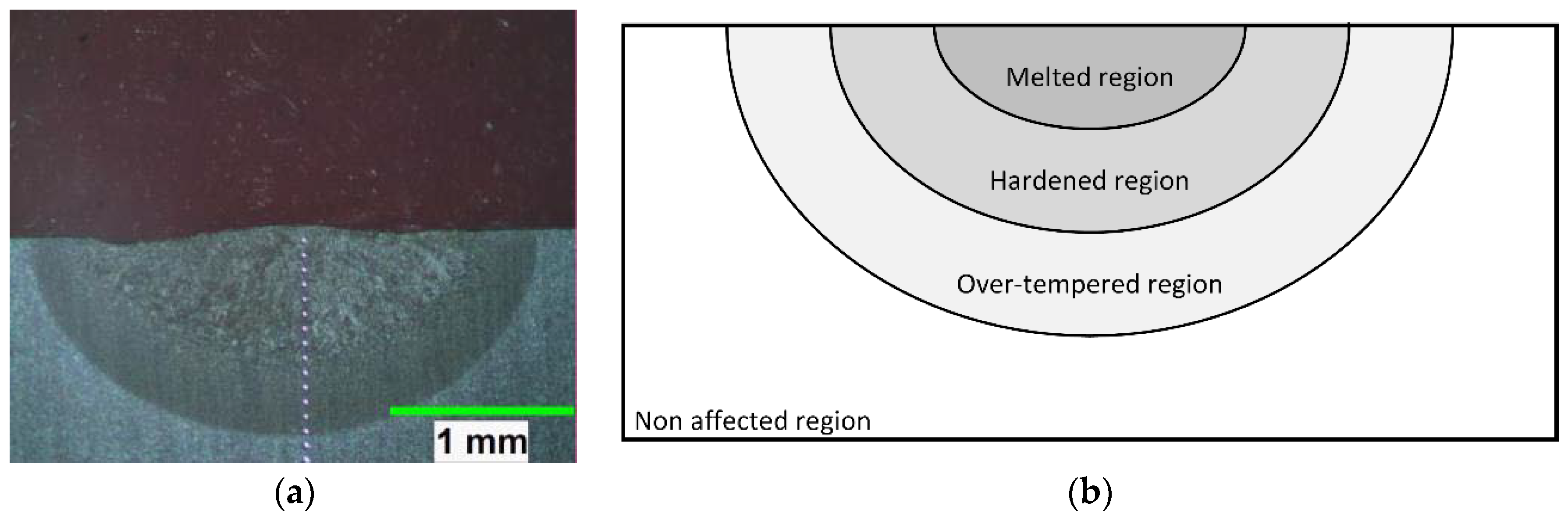
Surface hardening with a laser beam is a selective and a clean hardening technique widely employed on low and medium carbon steel, as is the induction heating process. The laser hardening process is characterized by its ability to provide specific treatment quality features, such as reduced distortion and cracking associated with through hardening of thick sections [3]. During the surface heat treatment, the surface layer of the hardened steel is exposed to a series of temperature variations due to the short process cycle time. As soon as the laser beam scans the mechanical part, the treated surface receives an amount of energy that can easily heat the surface layer beyond the austenitizing temperature Ac3. Figure 1a illustrates the metallographic cross-section image of an AISI 4340 steel plate hardened using a laser beam. In this example, the laser power was adjusted to 1 kW and the beam was scanned at 16 mm/s. The transformed region had an elliptical shape due to Gaussian distribution of the beam, which stipulates that the maximum energy be applied at the center of the spot. It is important to distinguish the both regions occurred in the transformed area that was affected greatly by the heat amount. As indicated in Figure 1b, the laser beam may melt the scanned surface, creating an area called the melted region; otherwise and in ordinary cases, steel’s self-quenching effect dramatically reduces the surface layer temperature from the austenitizing temperature Ac3 to the part’s interior temperature. This temperature gradient occurs in an extremely short period of time, forming a hardened region that contains hard, fine martensite and an over-tempered region between the hardened region and the material bulk that consists of tempered martensite with a small amount of retained austenite. The remaining region does not seem to be affected by the thermal flow during the laser hardening stage [4].
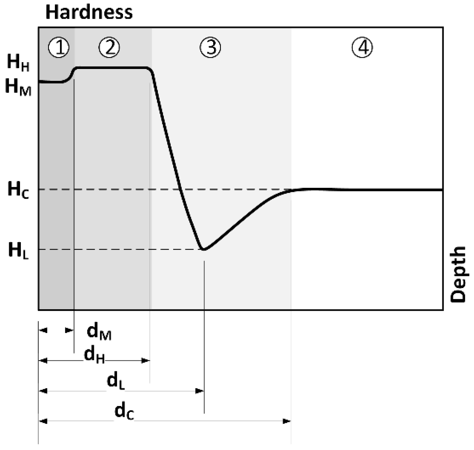
Many studies have featured the laser hardening process, the majority of which were experimental studies limited to examining the effect of process input parameters on the treated layer [5,6]. Other studies have focused on theoretical and analytical aspects, trying to understand and quantify the thermal and microstructural mechanism during the phenomenon [7]. These studies were often focused on the maximum hardness surface treated (HH), which constitutes an interesting response and does not reflect the full picture of treatment quality. A typical hardness curve obtained by laser hardening is illustrated in Figure 2. This curve is characterized by the melted layer (1). It also includes a hardened region (2) that records a high hardness value and is a homogeneous microstructure with nearly constant hardness and compressive residual stress levels. The over-tempered region (3) represents the hardness loss caused by a microstructural changes, and reaches minimum value. This region includes the hardness rise until it reaches the initial hardness value and is composed of a mixture of hard and over-tempered martensite since the temperature was between Ac1 and Ac3. The fourth region (4) records a constant hardness value that represents the tempered martensite constituting the initial microstructure in the part’s core before laser treatment. The LHQ is a feature that cannot be confined to a limited response, but rather a coherent set of response results depending strongly on process parameters. In addition to the hardness values HH, laser hardening quality can be also estimated through the depth of the four regions described previously, the melted region (dM), hardened region (dH), over-tempered region (dL) and total transformed region (dC). The hardness profile is a direct result of temperature distribution during and after heating and could greatly affect part distortion, martensite microstructure and compressive residual stresses resulting at the surface [8].
dM, dH, dC and HH can be controlled by input process parameters, so modeling these responses is a successful means of attaining the desired quality process while avoiding time and cost limitations. The modeling approach was the focus of several laser hardening or welding studies that were generally based on the artificial neural network (ANN) technique and the multi-regression method. Lambiase developed an expert model using the ANN technique to evaluate the temperature profile and temperature history of a laser-treated part under different processing conditions [9]. As a result, the measured hardness values showed relatively good correspondence with the predicted temperature profile. Woo used both multi-regression and artificial neural network techniques to develop models for assessing the hardened layer dimensions of SM45C steel, mainly the effect of coating thickness parameters [10]. Bappa highlighted the laser welding process by predicting welding quality [11]. His work aimed to establish a correlation between laser transmission welding parameters and output variables through a non-linear model based on artificial neural networks. After studying the effect of the process parameters on the responses of interest or LHQ, this study aims to develop models capable of predicting the hardness profile and controlling the LHQ according to input process parameters. The modeling technique is based mainly on the choice of modeled attributes. Hardness profile attribute characterization is a necessary step for modeling, so these attributes must provide a global representation of hardness profile behavior. Two different approaches were used during this study to characterize the hardness profile according to process parameters such as laser power and scanning speed. The extracted attributes were modeled using the artificial neural network based on multilayer perceptron (MLP). The generated models were analyzed using special evaluation criteria to determine the appropriate characterization approach for modeling the LHQ.
2. Experimental Aspect
2.1. Experimental Conditions
Steel heat treatment quality depends largely on the input factors. In the case of laser heat treatment, machine parameters such as laser beam power (PL) and scanning speed (VS) have the greatest effect and make the most significant contributions to the required results. All other parameters that were investigated in the relevant studies can be considered to have made fewer contributions when comparing laser beam power and scanning speed. The experimental aspect of this study was applying the laser heat treatment process to AISI 4340 steel to assess the parameters’ impact on the quality of the hardened layer. In addition to laser power and laser beam velocity, with four levels of each, the input parameters of the first experiment were restricted to initial steel hardness (HC) and surface roughness (Ra), with two levels of each. The power varied from 400 to 1300 W with a step of 300 W, while the speed varied from 10 to 40 mm/s with 10 mm/s incrementing. The initial hardness values were 40 and 50 HRC, and the surface roughness was tuned at 0.8 and 2.4 µm.
2.2. Experimental Design
A test plan that contains all possible combinations of all input factors is known as a fully crossed design and is considered the best approach for carrying out such experiments, based on its credible results. However, due to time and cost limitations, it is not widely used and only a few experiments have been carried out using a fully crossed design. Alternatively, the orthogonal arrays (OA) developed by Taguchi represent a judicious and robust fractional factorial design [12]. Used in most experimental studies similar to this paper, this strategy can achieve a high-quality level process while reducing the number of tests that are strictly necessary to collect all statistically significant data [13]. Based on the number of considered parameters and their levels, L16 orthogonal arrays were an adequate test strategy for this study, while L8 remained an appropriate choice for validation tests.
2.3. Experimental Set-Up
The steel used in this study was AISI 4340 parallelepiped plates (50 mm × 30 mm × 5 mm). The plates were subjected to several prior preparations, such as pre-heat treatment to achieve the desired initial hardness levels, as well as a plate surface texture preparation using CAMI-Grit-100 sandpaper with an average particle diameter of 140 µm to obtain a surface roughness (Ra) of approximately 2.4 µm and CAMI-Grit-200 sandpaper with an average particle diameter of 68 µm to obtain a surface roughness (Ra) of approximately 0.8 µm. The laser beam was provided by a Nd:YAG robotic cell, and the value range levels of machine parameters such as beam power and scanning speed were taken to ensure the complete austenitization of the steel layer during the heat treatment (Table 1). Once the treatment was performed, the hardness profile was characterized by using a Clemex microhardness measurement machine using 500 g load, which provided the hardness profile shape of each test. The hardness is evaluated first in HV and converted to HRC scale.
2.4. Experimental Results Analysis
Effective modeling relies overwhelmingly on the selection of parameters with the most influence on the phenomenon. For this reason, the statistical study of process results is required before modeling to determine the impact of the parameters and the contribution of each. Several statistical tools can be used, though the most frequently used is the analysis of variation (ANOVA). ANOVA analysis is a computational technique that reveals all the necessary information about the process parameters that can help determine the impact of each parameter and its contribution to the controlling response. Information provided by ANOVA analysis includes degrees of freedom, sum of squares, mean square, p-value and f-value; based on this information, the process parameters were ranked according to their importance in the experiment. The response surface methodology (RSM) model corresponding to the measured case depth (dH) was established according to the analytic methods depicted above. ANOVA analysis was performed with a stepwise mode, which automatically eliminate the insignificant terms. Table 2 presents the detailed statistical analysis confirming that f-value is important for almost all factors except the roughness surface and a p-value of less than 0.09. In this case, the laser power (PL), scanning speed (VS) and initial hardness (HC) were all significant model terms. Based on the ANOVA results, the parameters predominantly affecting the LHQ were laser beam power (52.76%) and beam scanning speed (32.92%). The contribution of initial hardness was less than 5%, and the factor related to surface roughness had no effect on the case depth in that situation. However, the contribution of the total error was about 8.73%. This result means that the process responses were somehow not controlled by the all-important input parameters. The coefficient of determination (R2) is mainly used to measure the relationship between experimental data and measured data. In this case, R2 was equal to 91.26%, proving a high correlation between experimental results and predicted results. The predicted R2 of 54.34% was in representative agreement with the adjusted R2 of 81.27%. Adequate precision measures the signal to noise ratio. The standard deviation related to the case depth prediction model was evaluated at 0.3201.
A similar experiment was performed with the same input parameters, except that the surface roughness parameter (Ra) was replaced by surface nature (SN). In this case, the first level correspond to the surface as initially treated and the second level is that obtained after machine tool finishing. Some similarities were noted regarding f-value and p-value concerning the analysis considering Ra. In fact, f-value was very important, exceeding 10 for the least significant factor (SN), and the p-value was less than 0.015 for SN again. It was also clear that PL has the largest effect on the response value, VS has less of an effect and HC has a little more effect. The three interaction terms affected the case depth less but were not ignored. This study allows for determination of the various effects and the ranking of each effect on the case depth (dH). Based on the data in Table 3, the variation in the three characteristics represents each parameter’s degree of influence on the response. It was confirmed by analyzing their contributions that PL affects dH by more than 58.66% and that VS contributes to the overall variation by more than 16%. The initial hardness influences the case depth by about 19% with an error of less than 2.5%. Most of the parameters were therefore taken into account during this study. It is important to note the non-presence of interactions between the four factors used in this study. The coefficient of determination (R2) was about 96.03%, proving a high correlation between experimental results and predicted results. The predicted R2 of 79.26% was in reasonable agreement with the adjusted R2 of 91.49%. Adequate precision measures the signal to noise ratio. The standard deviation related to the case depth prediction model was evaluated at 0.3240.
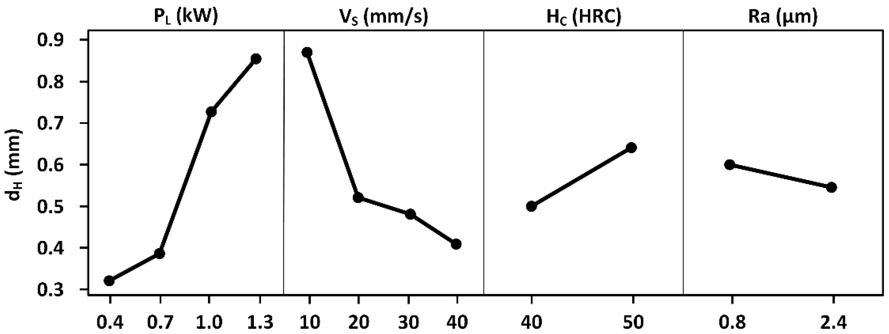
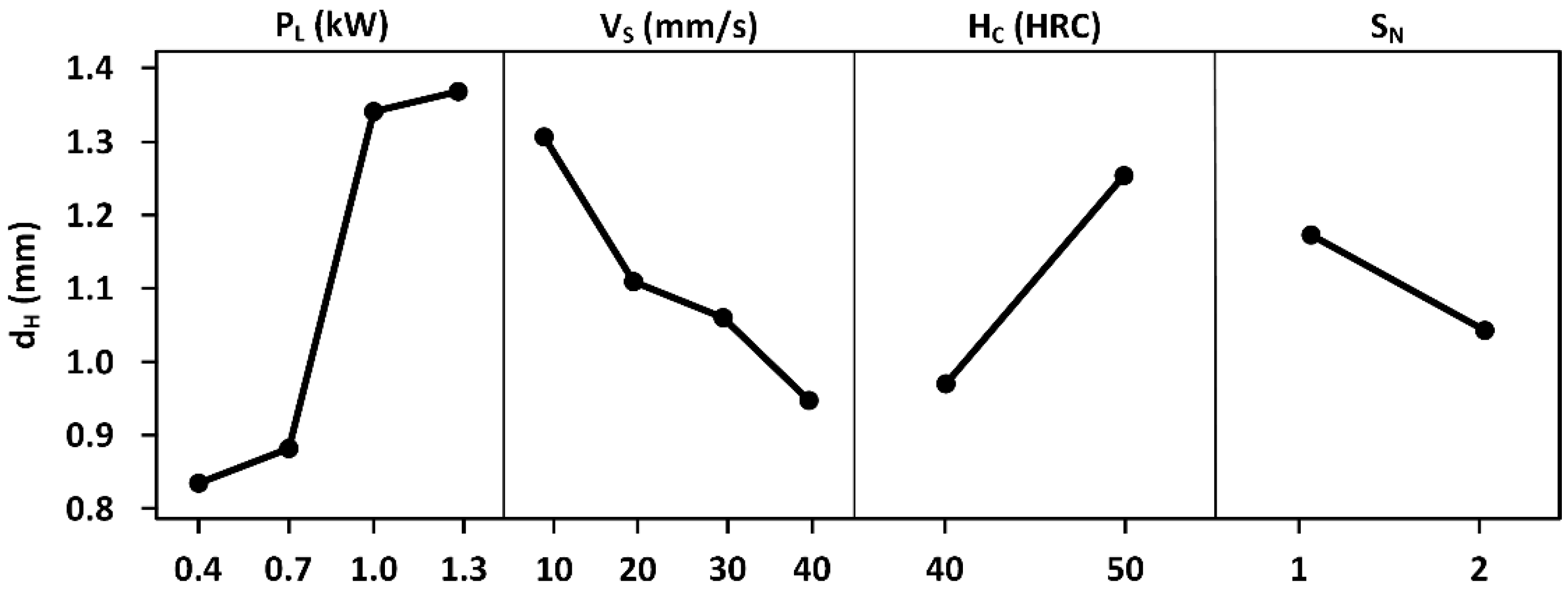
Figure 3 and Figure 4 present the average effect graphs certifying that the four parameters affected the case depth to different degrees. dH increased with power and initial hardness and decreased with speed and surface roughness. dH also increased with power and initial hardness and decreased with speed and surface nature. The drawn points match up to the averages of the observations for each factor level. These results confirm the relative importance of the contribution of different factors in the variation of dH. The effects of the four factors in both cases (Ra and SN) do not follow the same tendencies. Overall, the case depth recorded maximum values at 1.3 kW, 10 mm/s, 50 HRC and Ra of approximately 0.8 µm. However, the minimum value was recorded at 0.4 kW, 40 mm/s and 40 HRC when the surface roughness was adjusted to 0.8 µm. The case depth recorded maximum values at 1.3 kW, 10 mm/s and 50 HRC when the surface was treated. However, the minimum value was recorded at 0.4 kW, 40 mm/s and 40 HRC when the surface was polished.
The information above shows that the surface nature (SN) of the treated plate had a greater impact on dH and on the other output response than surface roughness (Ra). The error contribution of the second experiment, in which the surface nature was considered as a fourth input parameter, was relatively small compared to the first experiment. This proves that the second experiment considered the important parameters and that laser hardening quality is strongly controlled by these parameters compared to the first experiment. Since the error contribution was less when Ra was replaced by SN in the ANOVA analysis, the selection of PL, VS, HC and SN as input parameters is promising and constitutes an effective choice for LHQ element models. Consequently, elaboration process using the best selection of parameters based on its effect and contribution helps the modeling and the validation steps.
3. LHQ Assessment Model
Returning to the objective mentioned above, this study aims to develop potent laser hardening quality models allowing for accurate prediction of key quality elements such as dM, dH, dC and HH depending on the input variables using systematic and rigorous approaches. It is well known that the modeling process is based on two important pillars; the type and number of variables to include in the model and the technique used to develop the robust model. According to ANOVA results and as mentioned earlier, the error of modeling and validation due to process input variables is expected to be minimal in the present study, which guarantees the success of the first modeling pillar to some extent. Regarding development of the model approaches, which are generally divided into two categories, theoretical modeling is an undesirable modeling option because of the complexity of the phenomena and the lack of understanding of fundamental laser hardening process behavior. In this case, empirical modeling is an appropriate means of reaching the study’s objective. The advantage of using the empirical approach is its ability to develop robust models with easily available information on the variables to include in the model [14].
Two famous modeling techniques are used in the relevant studies. The first is the multivariate or multivariable regression method; the second, the artificial neural network technique, was used in this study. The artificial neural network technique was adopted because of its ability to model the identified elements according to large numbers of controlling variables, even if the relationship between the identified element and the variables is non-linear. ANN contains several types of networks, such as feedforward neural networks (FNN), radial basis function networks (RBF), Kohonen self-organizing networks (KSON), learning vector quantization (LVQ) and the most popular technique used, multilayer perceptron (MLP). The research performed by Arnaiz-Gonzalez et al. has allowed to test two types of artificial neural networks (multilayer perceptron and radial basis functions) applied to milling process using ball-end tool. The artificial neural networks (ANNs) are very useful due the complexity and the nature of the cutting task, and due to the high number of variables that affect greatly dimensional errors. The obtained results demonstrate that the radial basis functions have better prediction capacity and achieving a precision of 1.83 μm and a correlation coefficient of 0.897. The researchers have noted that ANNs can powerfully improve their performance with more experimental dataset and with various parameters [15].
In the present study, effective modeling is the result of a set of systematic and rigorous sequences that begin by carrying out the experimental tests according to a well-defined combination of variables (PL, VS, HC and SN). This combination of variables was proposed by Taguchi’s OAs (L16), which were included in the models. Once the tests were done, response result data collection for modeling began; the data collection was done using specific techniques that will be explained later in the paper. A statistical analysis procedure to determine the impact, contribution and relationship between the process input variables and the data collected was carried out while taking into account all the conditions that could influence the modeling. The crucial step in the modeling sequences was the choice of technique for modeling and performance criteria. Once this step has been completed, it will take time to train the generated models, followed by the performance evaluation [16]. Based on certain performance evaluation criteria such as mean square error (MSE), a comparative study was carried out to compare the model’s credibility and the accuracy of the modeled LHQ to that measured in this study.
Modeling Techniques
Two LHQ modeling techniques were used in this study. Both techniques have a relationship with the hardness profile curve and how it can be characterized. The first technique involves directly extracting certain points along which the hardness profile curve can be drawn. This technique is called the punctual approach (Figure 5); each point extracted from the curve contains an abscissa and ordinate (HM, dM), (HH, dH), (HL, dL) and (HC, dC). The coordinate values depend on the process input variables, and the variations in these points in relation to the process variables define hardened profile sensitivity. Modeling the hardness profile curve with this technique means that LHQ will also be modeled.
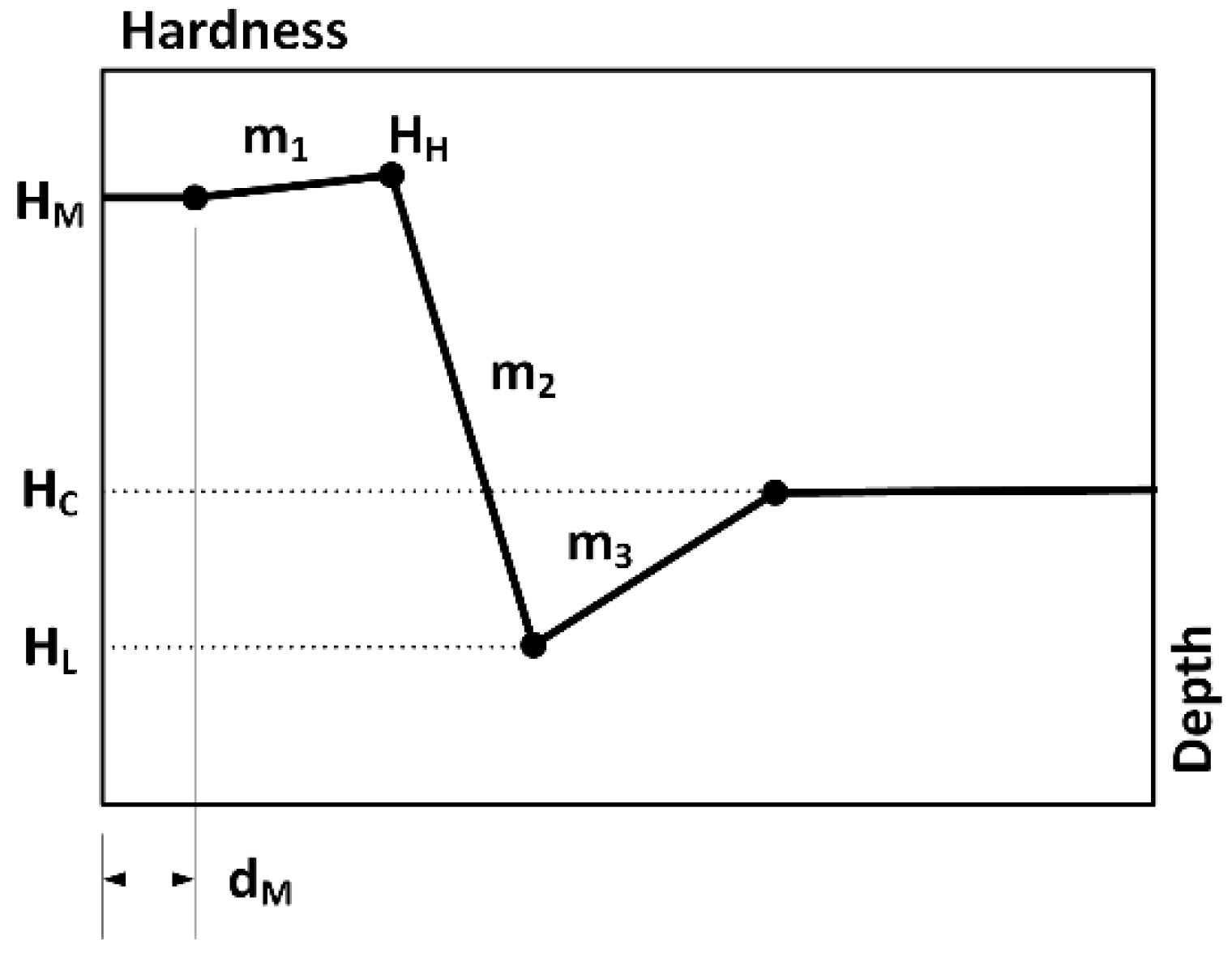
The second technique is called the geometrical approach. This technique extracts all amplitudes, slopes and peaks from the hardness profile curve that can provide an image of its shape, in which the mentioned attributes have a relationship with the LHQ. The ambiguous attributes considered in the geometrical approach are m1, m2 and m3, which represent the slopes, by means of which certain quality elements such as dH and dC can be calculated (Figure 6). m1 is the result of dividing the difference between HH and HM and the difference between dH and dM (Equation (1)). m2 is the result of dividing the difference between HL and HH and the difference between dH and dM (Equation (2)). m3 is the result of dividing the difference between HC and HL and the difference between dC and dL (Equation (3)). Note that the slopes m1 and m3 are positive and m2 is negative. Using these approaches to model the hardness profile is an effective way to model the LHQ. Otherwise, in this study, the LHQ modeling process is defined by dM, dH, dC and HH modeling.
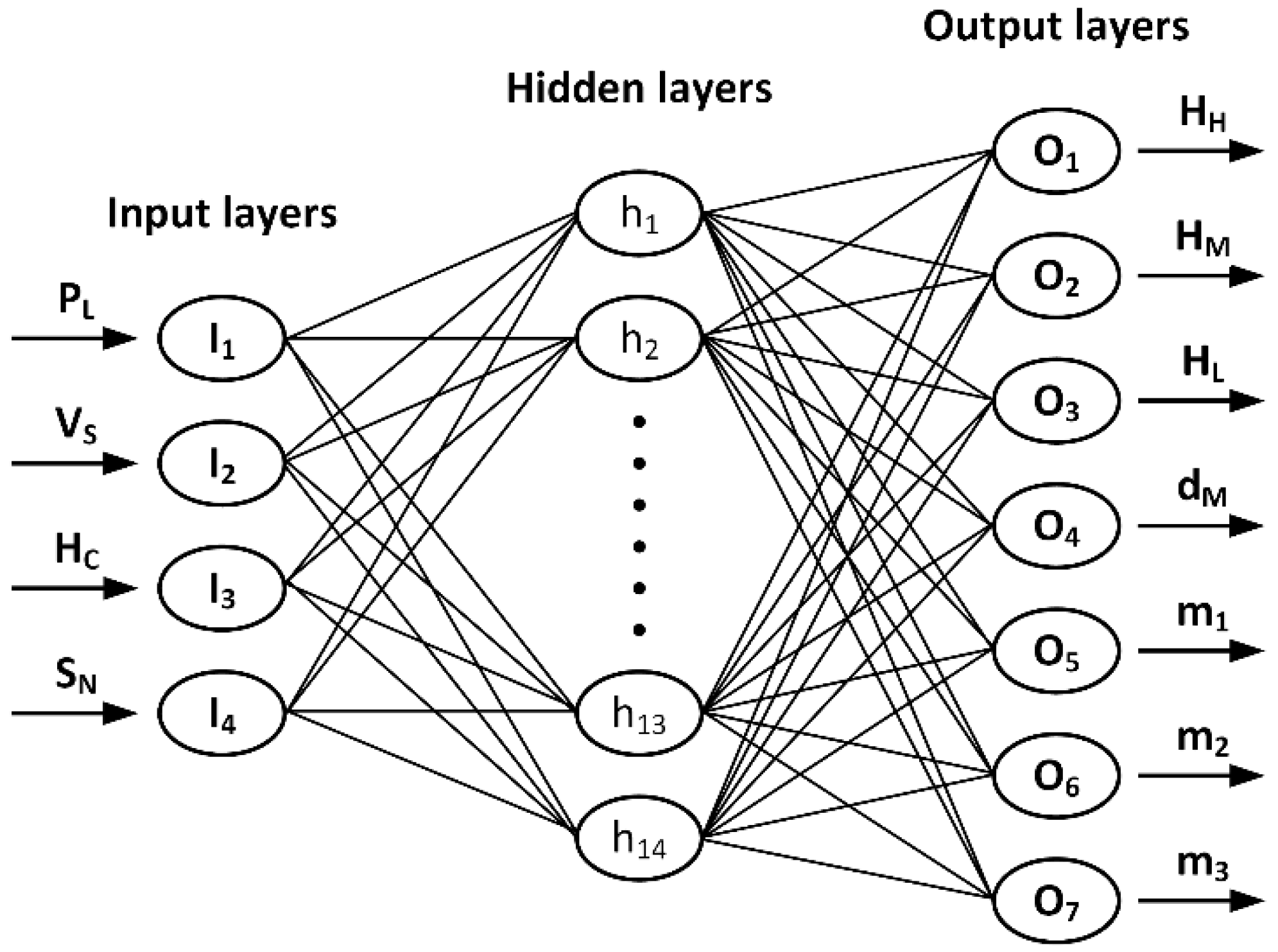
As was previously mentioned, the modeling process was performed using a multilayer perceptron (MLP) ANN technique that is known for its forecasting ability, simplicity and flexibility for modeling. MLP consists of three layers with each layer containing a certain number of neurons; the number of first- and third-layer neurons is equal to the input variables and number of modeling attributes, respectively. The second layer is the hidden layer. The modeling training performance depends on the size of this layer. To establish the size of the hidden layer, certain criteria must be taken into consideration, such as the number of input and output neurons and the complexity of the estimated parameters to evade the overfitting that can affect the model’s credibility and accuracy. After several training attempts, 12 neurons in the hidden layer met the best accuracy of generated models according to the assessment and performance criteria selected in the case of modeling punctual approach attributes (Figure 7). In the other case, and to generate geometrical attribute models with maximum accuracy, the best MLP architecture was with a hidden layer containing 14 neurons (Figure 8). While both the geometrical and punctual approaches based on MLP had the same number and nature of input variables, interpreting the difference in the number of neurons in the hidden layer may return to the complexity of the output variables so that adding two neurons to the hidden layer of the geometrical approach MLP when comparing it to the punctual geometric case MLP was the best solution for optimizing training performances.
4. Results and Discussion
The below tables present an assessment of the geometrical and punctual attribute models based on certain performance criteria. As is shown in the tables below, the mean absolute error (MAE), maximum relative error (XRE), mean square error (MSE) and total square error (TSE) were considered in this study. Table 4 and Table 5 show the results of the punctual and geometrical models by exhibiting MAE, XRE, MSE and TSE values. When using the geometrical approach, the convergence relationship between the modeled and eventual variables or MAE values were somewhat larger than when the punctual approach was used in both the training (T) and validation (V) tests cases.
The maximum relative errors or XRE of dM and HH models using the geometrical approach were less than the maximum relative errors of the punctual model, while the opposite is the case for HM and HL. Considerable values of XRE in m1 and m3, which represent the passage from (dM, HM) to (dH, HH) and from (dL, HL) to (dC, HC) respectively, can be explained by the HM and HL error effect while training models using ANN. Concerning m2, the XRE value was infinitely small due to the small size of the transition region compared to the corresponding hardness variation. The mean square error MSE and total square error TSE criteria provide the same information on model performances but with different values.
Table 6 summarizes all results concerning laser hardening modeling such as HH, dM, dH and dC. The mean absolute percentage error (MRE) is considered in order to evaluate the accuracy of the LHQ models and to compare the modeled attributes according to the characterization approach used to extract them. Using the geometrical approach, dH and dC were not included in the list of extracted attributes. dH and dC models were not generated directly, but were rather the result of modeling other attributes. Based on the MRE value, the results presented in Table 6 demonstrate that the laser hardening quality variable models present better accuracy when the geometrical approach was implemented; the difference is small.
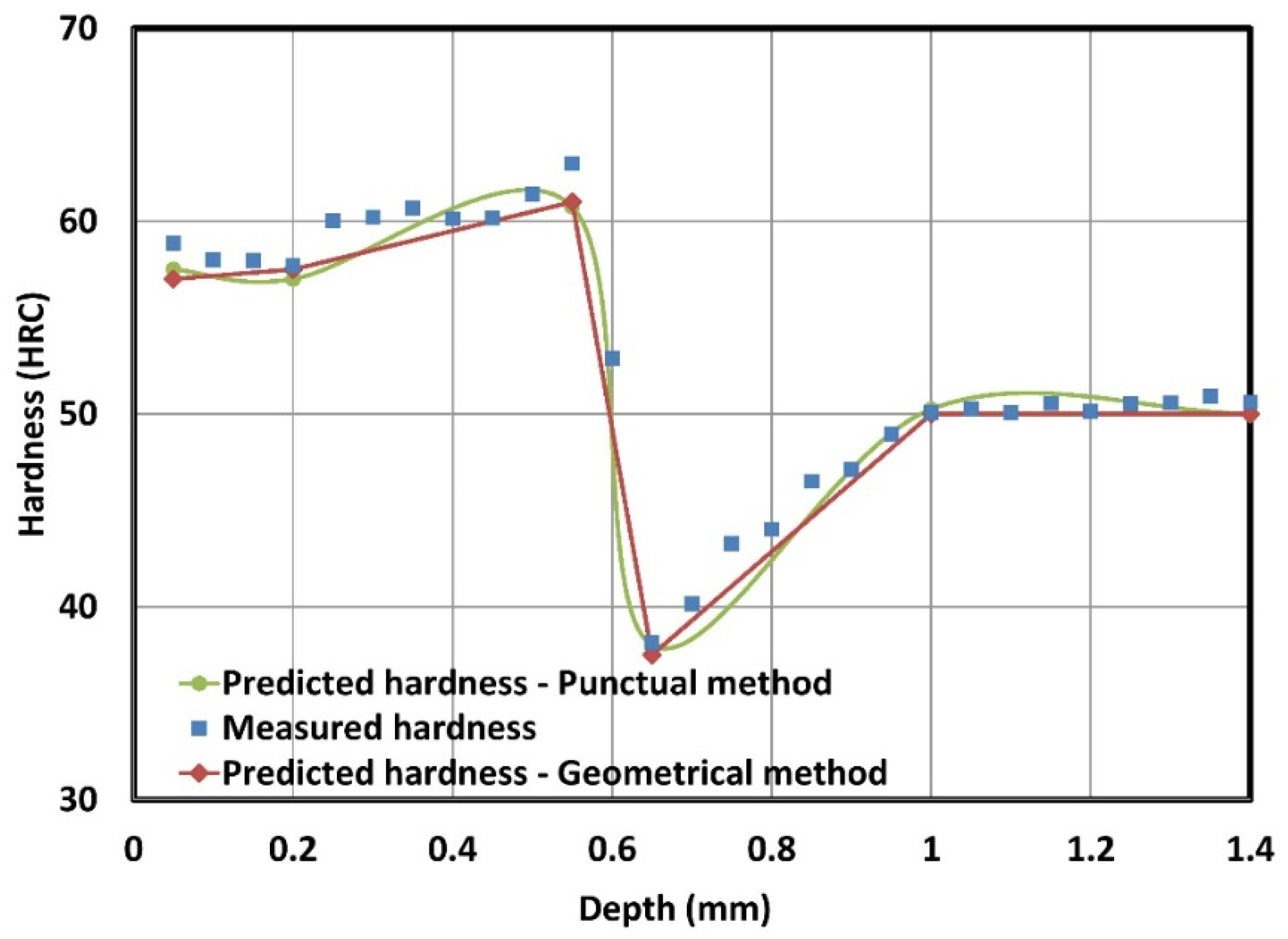
Figure 9 presents a comparison between the modeled LHQ elements through both approaches and the measured results. The figure contains three curves; the black curve represents the hardness profile (0.7 kW, 10 mm/s, 50 HRC and as-treated surface) while the other curves represent the modeled hardness profiles using the punctual approach and the geometrical approach. The peaks of the red curve match the corresponding point of the measured hardness profile. There is an extremely small difference between the measured hardness profile and the hardness profile provided by the punctual model. The results of these figures provide an idea for modeling the LHQ element using both the geometrical and the punctual approach and then deciding on the most appropriate modeling technique to obtain the best and most promising results. The hardness is measured initially in HV and converted to HRC.
5. Conclusions
- Laser hardening processing was performed on 4340 steel during which the parameters of laser power, beam scanning speed, initial hardness and surface roughness were considered and for which the testing strategy was designed according to the Taguchi method (OA). The analysis of variance indicated that the machine parameters (laser power and beam scanning speed, in order of importance) have the greatest impact on process quality, followed by initial hardness.
- The impact of surface roughness was quite low compared to the rest of the variables. By repeating the same experimental process and exchanging the surface roughness variable for surface nature, it was determined that for a certain defined interval, surface nature has more of an impact than surface roughness; the experiment’s total error contribution decreased when surface nature was used. The results of the experiment’s second process were considered for the modeling process in this study.
- Structured approaches were adopted to model the LHQ variables according to the second experiment parameters using a multilayer perceptron ANN calculation model. The generated models were evaluated through performance evaluation criteria, and the results allowed us to conclude the following. Modeling the extracted attributes from the hardness profile curve using both approaches is an ingenious way to model LHQ elements with excellent accuracy.
- According to the accuracy of the generated models, the geometrical attributes are the most appropriate variables for LHQ modeling, rather than the punctual attributes. However, both approaches proposed are effective techniques that provide promising LHQ models.
Author Contributions
Conceptualization, I.M., A.E.O and N.B.; Methodology, I.M., A.E.O and N.B.; Software, I.M.; Validation, I.M. and N.B.; Formal Analysis, I.M. and N.B.; Investigation, I.M., N.B. and A.E.O.; Resources, N.B. and A.E.O.; Data Curation, I.M.; Writing-Original Draft Preparation, I.M., N.B. and A.E.O.; Writing-Review & Editing, N.B. and A.E.O.; Visualization, I.M.; Supervision, A.E.O. and N.B.; Project Administration, I.M.; Funding Acquisition, N.B.
Funding
This research was funded by Natural Sciences and Engineering Research Council of Canada (Discovery Grants Program number RGPIN-2015-05978).
Conflicts of Interest
The authors declare no conflict of interest.
References
- Thomas, G.D.; Samuel, J.R.; Glenn, W.G. Heat Treatment and Properties of Iron and Steel; National Bureau of Standards Monograph 18, Supersedes Circular 495 and Monograph 18; National Bureau of Standards: Gaithersburg, MD, USA, 1966. [Google Scholar]
- Schneider, M.J.; The Timken Company; Chatterjee, M.S.; Bodycote. Introduction to Surface Hardening of Steels. In ASM Handbook, Volume 4A, Steel Heat Treating Fundamentals and Processes; Dossett, J., Totten, G.E., Eds.; ASM International: Almere, The Netherlands, 2013; pp. 389–398. [Google Scholar]
- Shang, H.M. On the width and depth of hardened zones during laser transformation hardening of tool steels. J. Mater. Proc. Technol. 1990, 23, 65–72. [Google Scholar] [CrossRef]
- Katsamas, A.; Zervaki, A.D.; Haidemenopoulos, G.N. Laser-beam surface transformation hardening of hypoeutectoid Ck-60 steel. Steel Res. Int. 1997, 68, 119–124. [Google Scholar] [CrossRef]
- Shiue, R.K.; Chen, C. Laser transformation hardening of tempered 4340 steel. Metall. Mater. Trans. A 1992, 23, 163–170. [Google Scholar] [CrossRef]
- Babu, P.D.; Buvanashekaran, G.; Balasubramanian, K.R. Experimental studies on the microstructure and hardness of laser transformation hardening of low alloy steel. Trans. Can. Soc. Mech. Eng. 2012, 36, 242–257. [Google Scholar] [CrossRef]
- Komanduri, R.; Hou, Z.B. Thermal analysis of the laser surface transformation hardening process. Int. J. Heat Mass Trans. 2011, 44, 2845–2862. [Google Scholar] [CrossRef]
- Grum, J.; Šturm, R. Laser surface melt-hardening of gray and nodular irons. Appl. Surf. Sci. 1997, 109, 128–132. [Google Scholar] [CrossRef]
- Lambiase, F.; Di Ilio, A.M.; Paoletti, A. Prediction of Laser Hardening by Means of Neural Network. In Proceedings of the 8th CIRP Conference on Intelligent Computation in Manufacturing Engineering, Ischia, Italy, 18–20 July 2012; pp. 181–186. [Google Scholar]
- Woo, H.G.; Cho, H.S. Estimation of hardened layer dimensions in laser surface hardening processes with variations of coating thickness. Surf. Coat. Technol. 1998, 102, 205–217. [Google Scholar] [CrossRef]
- Acherjee, B.; Mondal, S.; Tudu, B.; Misra, D. Application of artificial neural network for predicting weld quality in laser transmission welding of thermoplastics. Appl. Soft Comput. 2011, 11, 2548–2555. [Google Scholar] [CrossRef]
- Hitchens, D.M.W.N.; Clausen, J.; Fichter, K. Asian Productivity Organization. In International Environmental Management Benchmarks; Springer: Berlin/Heidelberg, Germany, 1999. [Google Scholar]
- Mason, R.L.; Gunst, R.F.; Hess, J.L. Statistical Design and Analysis of Experiments: With Applications to Engineering and Science; John Wiley & Sons: Hoboken, NJ, USA, 2003. [Google Scholar]
- Alberdi, A.; Rivero, A.; López de Lacalle, L.N.; Etxeberria, I.; Suárez, A. Effect of process parameter on the kerf geometry in abrasive water jet milling. Int. J. Adv. Manuf. Technol. 2010, 51, 467–480. [Google Scholar] [CrossRef]
- Arnaiz-González, Á.; Fernández-Valdivielso, A.; Bustillo; López de Lacalle, L.N. Using artificial neural networks for the prediction of dimensional error on inclined surfaces manufactured by ball-end milling. Int. J. Adv. Manuf. Technol. 2016, 83, 847–859. [Google Scholar] [CrossRef]
- El Ouafi, A.; Belanger, R.; Guillot, M. Dynamic resistance based model for on-line resistance spot welding quality assessment. Mater. Sci. Forum 2012, 709–709, 2925–2930. [Google Scholar] [CrossRef]
Figure 1.
Metallographic cross-section of the hardened region (a) and representation of a typical cross-section of a laser-hardened plate (b).
Figure 1.
Metallographic cross-section of the hardened region (a) and representation of a typical cross-section of a laser-hardened plate (b).

Figure 2.
Representation of LHQ elements through the hardness profile curve.

Figure 3.
Parameter effects (including surface roughness Ra) on dH.

Figure 4.
Parameter effects (including surface nature S) on dH.

Figure 5.
Punctual technique for extracting attributes.

Figure 6.
Geometrical technique for extracting attributes.

Figure 7.
Punctual ANN model architecture.

Figure 8.
Geometrical ANN model architecture.

Figure 9.
Measured and predicted hardness profile curves.


Table 1.
Scratching parameters of the process and their levels.
| Parameters | Levels |
|---|---|
| Power (kW) | 0.4, 0.7, 1.0 and 1.3 |
| Speed (mm/s) | 10, 20, 30 and 40 |
| Initial hardness (HRC) | 40, 50 |
| Surface roughness (µm) | 0.8, 2.4 |
Table 2.
ANOVA results for factors including Ra.
| Source | DF | Sum of Squares | Mean Square | f-Value | p-Value | Contributions (%) |
|---|---|---|---|---|---|---|
| PL (kW) | 3 | 0.81125 | 0.27042 | 14.09 | 0.002 | 52.76 |
| VS (mm/s) | 3 | 0.50625 | 0.16875 | 8.79 | 0.009 | 32.92 |
| HC (HRC) | 1 | 0.07562 | 0.07562 | 3.94 | 0.088 | 4.91 |
| Ra (µm) | 1 | 0.01000 | 0.01000 | 0.52 | 0.494 | 0.65 |
| Error | 7 | 0.13437 | 0.01920 | – | – | 8.73 |
| Total | 15 | 1.53750 | – | – | – | 100 |
Table 3.
ANOVA results for factors including SN.
| Characteristic | DoF | Sum of Squares | Mean Square | f-Value | p-Value | Contributions (%) |
|---|---|---|---|---|---|---|
| PL (kW) | 3 | 0.94092 | 0.31364 | 55.94 | 0 | 58.66 |
| VS (mm/s) | 3 | 0.25717 | 0.08572 | 15.29 | 0.002 | 16.03 |
| HC (HRC) | 1 | 0.30526 | 0.30525 | 54.45 | 0 | 19.03 |
| SN | 1 | 0.06126 | 0.06125 | 10.93 | 0.013 | 3.81 |
| Error | 7 | 0.03924 | 0.00560 | – | – | 2.47 |
| Total | 15 | 1.60384 | – | – | – | 100 |
Table 4.
Model performance criteria summary using the punctual approach.
| Variables | MAE | XRE | MSE | TSE | ||||
|---|---|---|---|---|---|---|---|---|
| T | V | T | V | T | V | T | V | |
| HH | 0.219 | 0.0640 | 1.149 | 0.497 | 0.0801 | 0.022154 | 1.2816 | 0.022154 |
| HM | 0.2656 | 0.1234 | 1.1 | 0.7709 | 0.099818 | 0.046141 | 1.5971 | 0.415267 |
| HL | 0.2219 | 0.0816 | 0.893 | 0.5932 | 0.0689 | 0.035358 | 1.1026 | 0.318228 |
| dM | 0.0131 | 0.0098 | 0.075 | 0.0493 | 0.000315 | 0.000187 | 0.00505 | 0.001688 |
| dH | 0.0295 | 0.012 | 0.141 | 0.0626 | 0.00138 | 0.000374 | 0.02208 | 0.003367 |
| dL | 0.0386 | 0.0117 | 0.173 | 0.0605 | 0.002342 | 0.000264 | 0.03747 | 0.002384 |
| dC | 0.0303 | 0.0065 | 0.137 | 0.0258 | 0.001444 | 0.000006 | 0.02311 | 0.000539 |
Table 5.
Model performance criteria summary using the geometrical approach.
| Variables | MAE | XRE | MSE | TSE | ||||
|---|---|---|---|---|---|---|---|---|
| T | V | T | V | T | V | T | V | |
| HH | 0.1529 | 0.05290 | 0.81 | 0.3248 | 0.040455 | 0.008447 | 0.647286 | 0.076024 |
| HM | 0.2465 | 0.09083 | 1.56 | 0.3969 | 0.148896 | 0.013468 | 2.382342 | 0.121213 |
| HL | 0.2068 | 0.24019 | 1.14 | 1.4457 | 0.081355 | 0.154602 | 1.301689 | 1.391424 |
| dM | 0.0094 | 0.00844 | 0.06 | 0.0463 | 0.000191 | 0.000179 | 0.003058 | 0.001618 |
| m1 | 0.5264 | 0.41324 | 2.35 | 1.7062 | 0.411062 | 0.321390 | 6.577006 | 2.892513 |
| m2 | 0.00034 | 0.00031 | 0 | 0.0020 | 1.95 × 10⁻⁷ | 2.57 × 10⁻⁷ | 3.12 × 10⁻⁶ | 2.83 × 10⁻⁷ |
| m3 | 0.49373 | 0.25813 | 2.31 | 1.0456 | 0.359161 | 0.106389 | 5.746584 | 0.957505 |
Table 6.
Geometrical and punctual model MRE comparison.
| Q-Element | Geometrical Approach | Punctual Approach | |
|---|---|---|---|
| T | HH | 0.2537 | 0.3626 |
| dM | 3.7599 | 5.1309 | |
| dH | 0.9377 | 4.7073 | |
| dC | 0.9425 | 3.0091 | |
| V | HH | 0.08836 | 0.1080 |
| dM | 2.77873 | 3.1369 | |
| dH | 0.73379 | 1.9079 | |
| dC | 1.29508 | 0.6520 | |
© 2018 by the authors. Licensee MDPI, Basel, Switzerland. This article is an open access article distributed under the terms and conditions of the Creative Commons Attribution (CC BY) license (http://creativecommons.org/licenses/by/4.0/).
Share and Cite
MDPI and ACS Style
Maamri, I.; Barka, N.; El Ouafi, A. ANN Laser Hardening Quality Modeling Using Geometrical and Punctual Characterizing Approaches. Coatings 2018, 8, 226. https://doi.org/10.3390/coatings8060226
AMA Style
Maamri I, Barka N, El Ouafi A. ANN Laser Hardening Quality Modeling Using Geometrical and Punctual Characterizing Approaches. Coatings. 2018; 8(6):226. https://doi.org/10.3390/coatings8060226
Chicago/Turabian StyleMaamri, Ilyes, Noureddine Barka, and Abderrazak El Ouafi. 2018. "ANN Laser Hardening Quality Modeling Using Geometrical and Punctual Characterizing Approaches" Coatings 8, no. 6: 226. https://doi.org/10.3390/coatings8060226
Note that from the first issue of 2016, this journal uses article numbers instead of page numbers. See further details here.