1. Introduction
Modeling and simulation of composites during an impact event is a huge challenge given the wide variety of composites and the associated complexity in characterization of the behavior of the constituent materials as well as the interaction between them. While composites have been in use for decades in a variety of industries such as civil structures, automotive and aerospace, building a predictive model is still daunting. Kaddour et al. [
1] list some of the challenges facing the industry. They include (a) shorter life cycles, (b) automated manufacture, (c) production of high volumes, (d) integrating 3D structures into 3D architectures, (e) development of alternative materials, and (f) meeting climate change targets. In the United States, several governmental agencies (including NASA and the FAA) have recognized the importance of building a framework for composites system by forming a public–private consortium. A press release [
2] states that “NASA formed the consortium in support of the Advanced Composites Project, which is part of the Advanced Air Vehicles Program in the agency’s Aeronautics Research Mission Directorate. The project’s goal is to reduce product development and certification timelines by 30 percent for composites infused into aeronautics applications.” A major reason for these challenges is the lack of mature material models that should be able to predict, with some degree of certainty, the deformation, damage and failure of composite systems.
Several approaches can be used to develop such numerical models. Vaziri et al. [
3] categorize the continuum mechanics approaches into four groups—(i) nonlinear elasticity theories; (ii) damage theories coupled with elasticity; (iii) classical incremental plasticity theory; and (iv) endochronic plasticity theory. Examples of these approaches and models can be found in [
4,
5,
6,
7,
8,
9]. From the viewpoint of engineering design, models should be driven with varying levels of input depending on the complexity of the composite so that the material model can be tailored for the required response. Currently, however, many material models are driven entirely by a few sets of material properties capturing orthotropic deformation and damage behavior. These include Young’s moduli, Poisson’s ratios, shear moduli, failure strain, and reduction factors for the strength of constituent parts (fibers) based on the failure of other constituent parts (matrix). Others require additional parameters to characterize failure using classical failure theories at the macroscopic level, e.g., Chang–Chang or Tsai–Wu, or a mixture of macroscopic level and local (fiber/matrix) driven failure, e.g., Hashin. This type of approach leads either to models with only a few parameters, which provide a crude approximation at best to the actual stress–strain curve, or to models with many parameters which require a large number of complex tests to characterize [
12]. Often, the lack of flexibility or sophistication in these models require that designers adjust the values of some of the model parameters using data from full-scale structural tests.
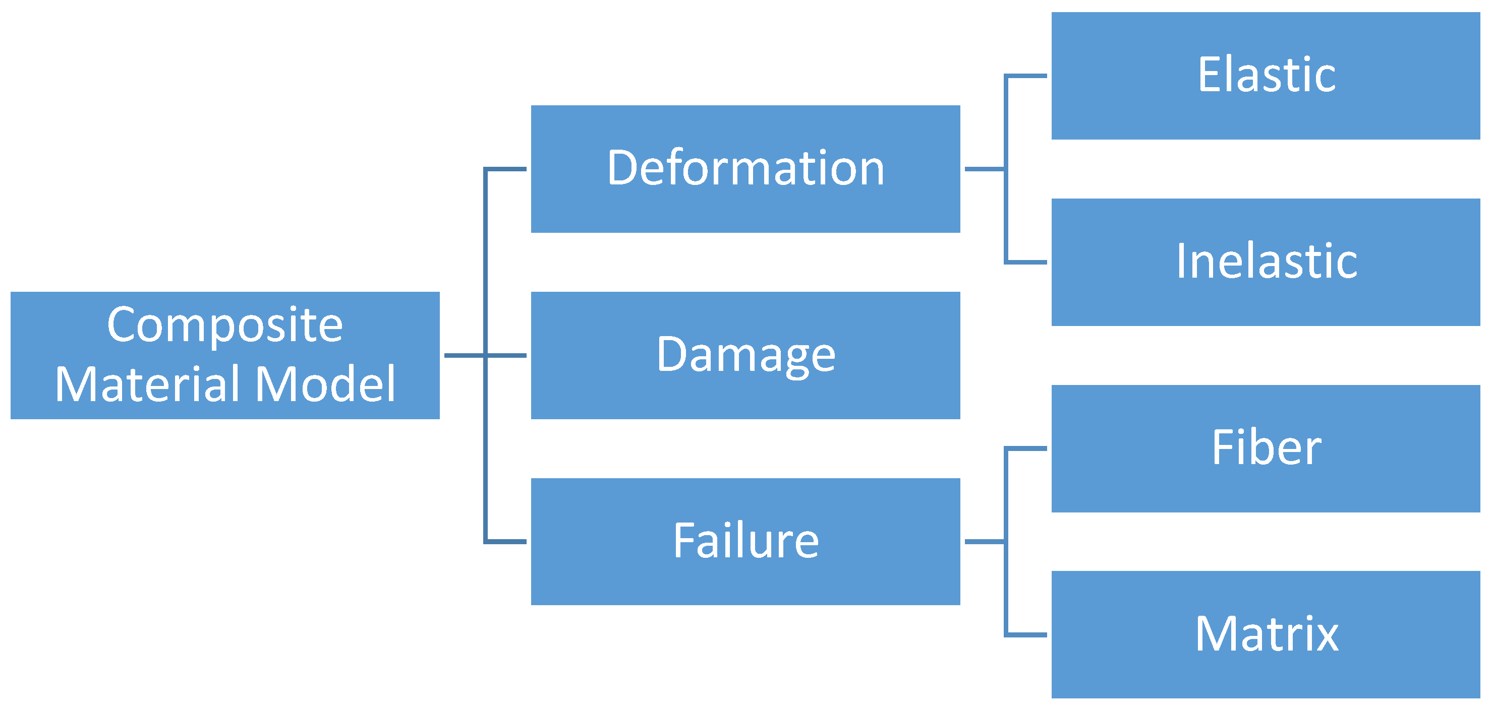
In the present approach, the composite impact model is divided into a deformation model, a damage model and a failure model (
Figure 1). Such a partitioning allows for the elastic and plastic deformations to be captured by the deformation model and the reduction in stiffness to be captured by the damage model. In other words, the deformation model simulates the nonlinear material response of the composite (due to either deformation or damage mechanisms), and the damage model simulates the nonlinear unloading due to stiffness reduction. The macroscopic tabulated failure model captures failure and does not rely on characterization of mechanisms leading to failure. The response of a system can then be monitored as the finite element calculations are processed through the deformation and damage models so that the failure model can be used to carry out failure predictions. The deformation model generalizes the Tsai–Wu failure criteria. A non-associative flow rule is used and the yield surface is based on strain-hardening orthotropic yield function. A strain equivalent formulation is utilized in the damage model that permits the plasticity and damage calculations to be uncoupled and captures the nonlinear unloading and local softening of the stress–strain response. A diagonal damage tensor is defined to account for the directional-dependent variation of damage. However, in composites, it has been found that loading in one direction can lead to damage in multiple coordinate directions [
19]. To account for this phenomenon, the terms in the damage matrix are semi-coupled as explained later. The overall framework is driven by experimentally obtained tabulated temperature- and rate-dependent stress–strain data as well as data that characterizes the damage matrix and failure [
13].
This paper discusses the details of the orthotropic elasto-plastic constitutive model. The current version supports solid finite elements with plans to extend the support to shell elements. The theoretical and implementation details are followed by numerical studies using a custom version of LS-DYNA where the constitutive model is implemented as MAT213. A commonly used unidirectional laminate, T800/F3900 graphite/epoxy composite, is used in the numerical studies.
2. Theoretical Details
The developed constitutive model is designed to model composites under impact loading. The input to the model consists of 12 tabulated stress–strain curves generated from actual experimental or virtual tests [
10]—1, 2 and 3-direction tension curves, 1, 2 and 3-direction compression curves, 1-2, 2-3 and 3-1 plane shear curves, and 45° off-axis tension/compression curves in the 1-2, 2-3 and 3-1 planes. A brief summary of the deformation model is presented here and further details can be found in our earlier publications [
11,
12,
13]. The yield function is a modified form of the commonly used Tsai–Wu composite failure model and is defined as
where
. The yield function coefficients,
, depend on the current yield stress values and are calculated as
where the superscripts
T,
C and 45 denote data obtained from tension, compression and 45-degree off-axis tests, respectively. A non-associative flow rule is used to compute the evolution of the components of plastic strain and the plastic potential function is defined as
where the
terms are a set of constant coefficients which are functions of the plastic Poisson ratios, with the coefficients defined as input parameters in the model.
2.1. Non-Associated Plastic Flow
Classical plasticity theory using associated plasticity assumes that the increment of plastic strain is normal to the yield surface, where the plastic potential function is defined as
based on Drucker’s stability postulate which works well for metals [
14] (where
is the plastic strain rate,
is the plastic multiplier,
is the yield function and
is the stress tensor in Voigt notation). However, associated plasticity is not ideal for most composites with various degrees of plastic anisotropy. For example, some composites exhibit linear elastic behavior in one or more directions, e.g., a unidirectional composite when loaded in the fiber direction. This would indicate that there is no plastic flow, or plastic strain accumulation with respect to the fiber direction. However, the yield function in Equation (1) cannot accommodate this. Thus, non-associated plasticity is required in creating a generalized composite material model as the flow law coefficients for the non-associated plastic potential function can be determined independently from the yield function terms. Mathematically, this situation (that associated plasticity cannot be used) can be described as follows. Consider an isotropic Tsai-Wu flow rule:
where
is the von Mises stress and
is the pressure. The condition for the uniaxial tension case can be derived as follows (
is the deviatoric stress):
Assuming that the linear term is zero, the plastic Poisson’s ratio can be derived as
Equation (13) shows that the plastic Poisson’s ratio can assume any value which is non-physical. Hence a non-associative flow rule is appropriate for the problem under consideration in this paper and is given by
where
is the plastic potential function.
2.2. Flow Rule and Determination of Flow Rule Coefficients
The deformation model uses a flow surface that is defined to determine the plastic flow direction (flow rule) as shown in Equation (14). In the plastic potential function (Equation (6)), the
terms are the flow rule coefficients, assumed to be constant, and
are the current stress values. To accurately represent the plastic flow of the material, the flow rule coefficients are calculated directly using the experimental data. Six of the coefficients are determined from unidirectional testing of the composite in the three principal material directions. In each case, the plastic potential function can be simplified resulting in set of functions from which the plastic Poisson’s ratios,
can be computed as
where
are the plastic strain rate components. It should be noted that since the plastic strains and their ratios are constantly changing, the average values are used in computing the coefficients. An examination of the ratios (the ratios compare the degree of plasticity in each material direction) in Equation (15) shows that the flow rule coefficients are not linearly independent. This requires that one of the flow rule coefficients be assumed. Usually the direction with the most plasticity is chosen and the flow rule coefficient value is assumed, e.g.,
. The stress–strain curve in that direction is tagged as the “master” curve. As an example, consider
. This results in the following simplified equations.
Similarly, assuming the 2-direction as the master curve,
, and
The first six flow rule coefficients are calculated with the experimentally obtained plastic Poisson’s ratios depending on the identified master curve. The final three terms –
,
and
must be calculated differently. These terms are calculated by fitting the shear curves with the master curve in the effective stress versus effective plastic strain space. This can be achieved by minimizing the difference between the master curve and shear curves, thus determining the optimal
H value. The optimal flow rule coefficient value,
, is obtained by computing the difference between the two curves and the problem is posed as a least-squares problem:
such that
where
n is the number of data points in the master curve,
is the
kth effective stress value from the master curve and
is the effective stress value from the shear curve. An alternative process for calculating these final three coefficients is available as fitting the off-axis curves to the master curve instead of the shear curves [
15].
2.3. Modeling Damage
Damage in composite material models is usually used to track the progression of micro-cracking. The continuum damage model developed by Matzenmiller et al. [
16] uses the initiation and accumulation of damage to model the nonlinear response of a composite by implementing damage parameters to reduce the effective stiffness of the material in a particular coordinate direction. The full damage tensor can be used to relate the true stress to the effective stress as
However, this full matrix is rarely employed. Typically, damage models use a diagonal damage tensor and assume that the components are a function of a single plastic strain, e.g.,
. However, in the current work, a semi-coupled, directional-dependent relationship, e.g.,
indicating that the components are functions of plastic strains in multiple directions, is used to construct the modified relationship as
The damage parameter
is defined as a function of the plastic strain and represents damage in
kl due to loading along
ij. By assuming that normal damage is due to all normal and shear terms, and shear damage is also due to all normal and shear terms, the damage model terms in Equation (21) can be expressed explicitly as
Since even the simplified form shown in Equations (21)–(22) is rather complex, one must carry out damage related testing to see how many of these terms are really necessary to characterize the damage of a specific composite. Determining the damage parameters requires the measurement of either the damaged modulus or plastic strain (by unloading the material to a state of zero stress) at several total strain values. One approach to using the experimental data is to compute the damaged modulus as shown in Equation (23) for the normal stress–strain relationship in the 11 direction.
where
is the damaged modulus of elasticity in the 1-direction, and
is the undamaged modulus of elasticity. This approach makes it possible to create a simple damage wrapper around the deformation model and details can be found in [
13,
19].
The theory as described in this section, is implemented in a special version of LS-DYNA as material model 213 (MAT213) and is used in the numerical studies.
3. Experimental and Numerical Modeling Studies
An impact test (LVG905) was conducted at National Aeronautics and Space Administration’s Glenn Research Center to validate the developed model [
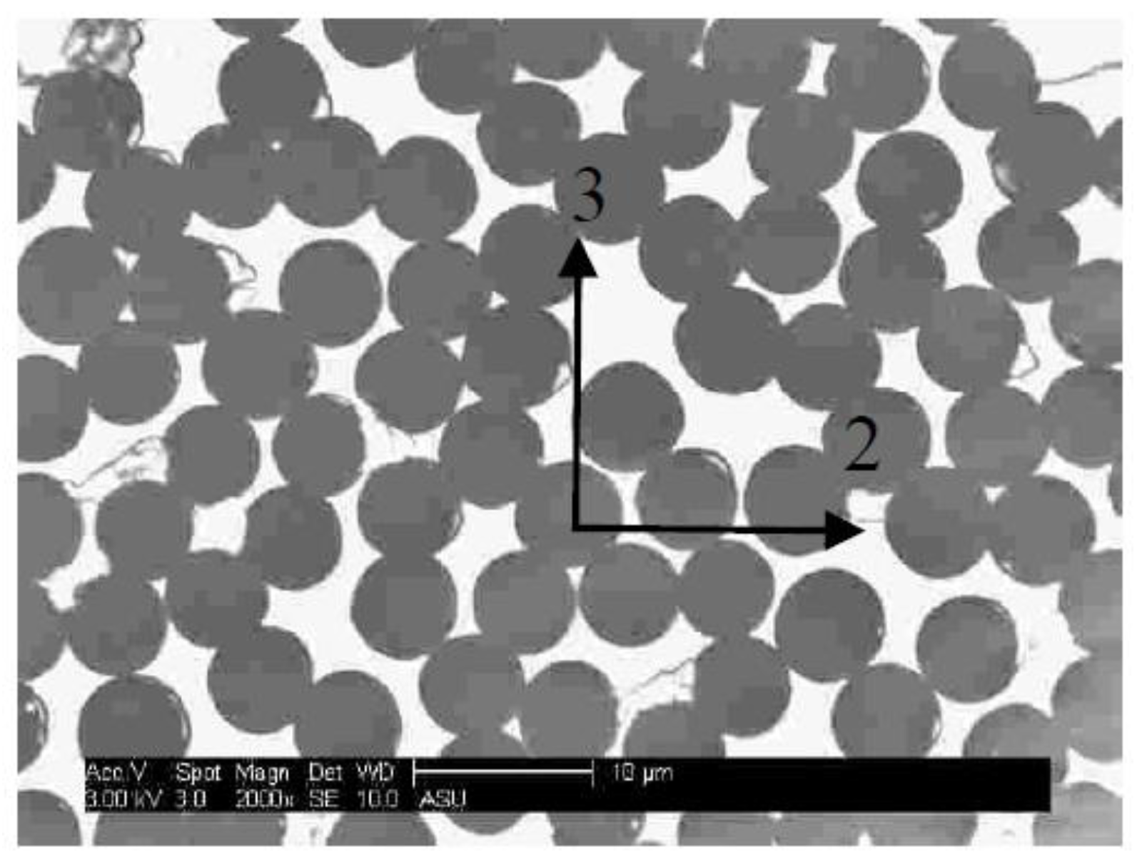
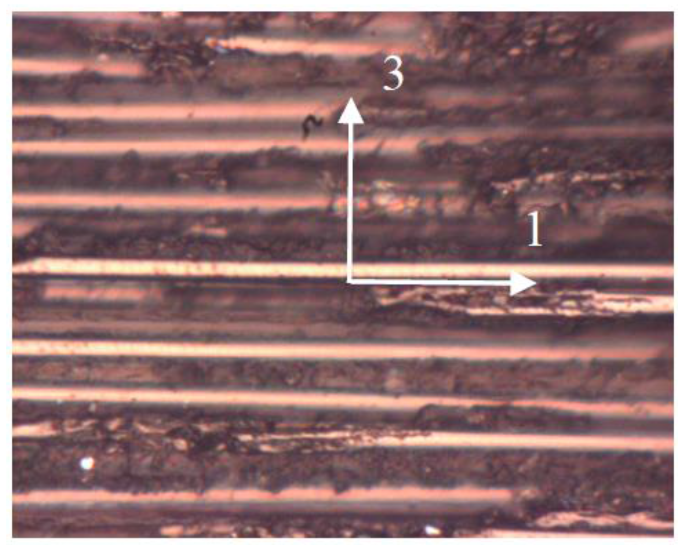
12]. The test involves a 30.48 cm × 30.48 cm × 0.3099 cm (12 in × 12 in × 0.122 in) thick composite flat panel subjected to a low velocity impact. The panel is made of T800S/3900-2B[P2352W-19] BMS8-276 Rev-H-Unitape fiber/resin unidirectional composite [
17]. Toray describes T800S as an intermediate modulus, high tensile strength graphite fiber. The epoxy resin system is labeled F3900 where a toughened epoxy is combined with small elastomeric particles to form a compliant interface or interleaf between fiber plies to resist impact damage and delamination [
17]. Magnified views of the composite are shown in
Figure 2 and
Figure 3.
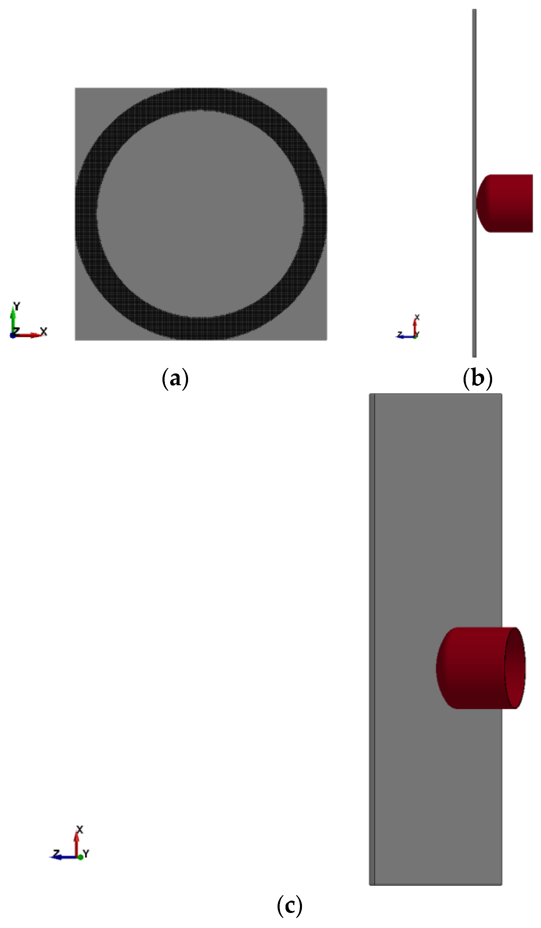
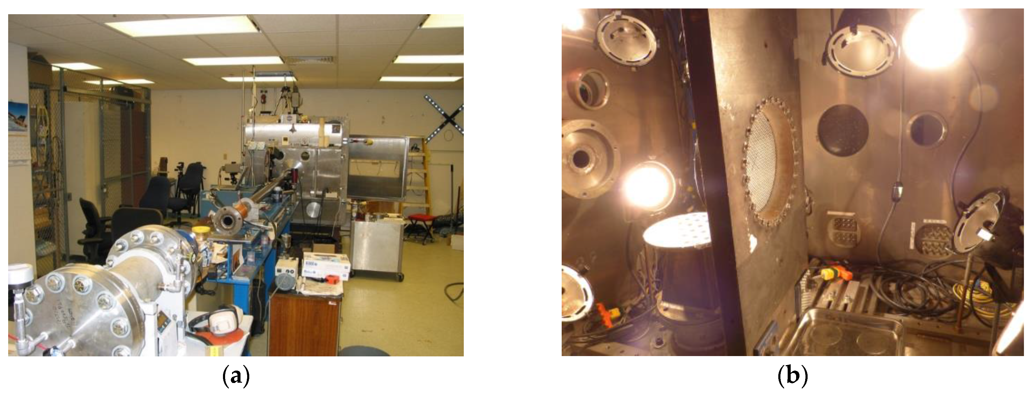
The schematics of the impact test are shown in
Figure 4a,b.
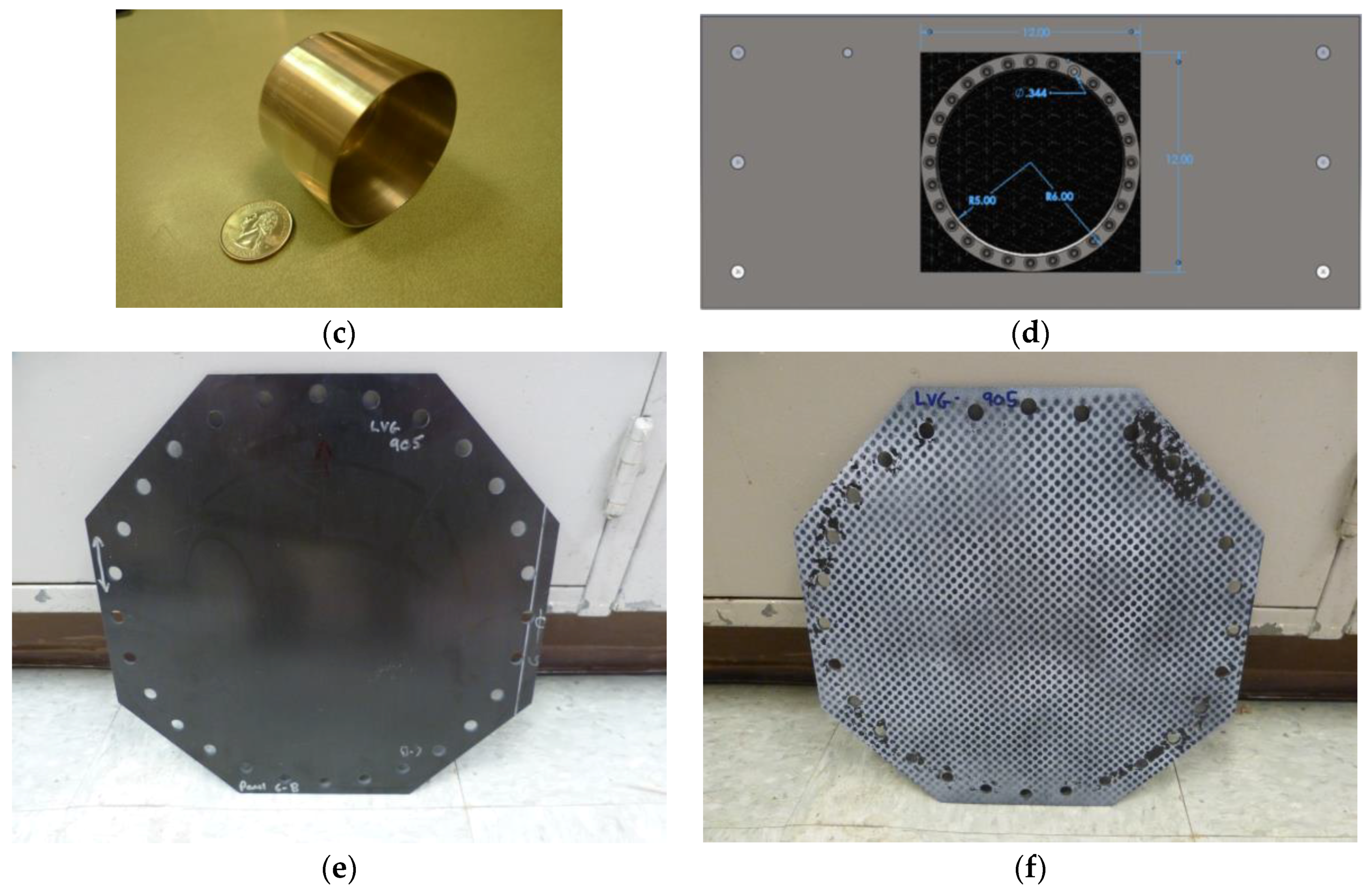
Figure 4c shows the 50.8 gm (0.112 lbm) hollow Al-2024 projectile with radiused front face.
Figure 4d shows the drawing of the panel and the support plate. The unidirectional panel was fabricated with 16 plies with the fibers in the panel oriented vertically corresponding to the Y-direction in
Figure 5a.
Figure 4e,f shows the panels before and after impact (no visible damage and cracks were observed). Each panel was tested before the impact test using ultrasound techniques (pulse echo scans with the sample immersed in water, a 5 MHz focused transducer was used using 1 mm scan and step increment) to determine if there were any initial damage or flaws. The tests revealed no flaws or damage. Digital Image Correlation (DIC) data was gathered from high-speed cameras and analyzed to yield full-field displacements and strains. It should be noted that the impact velocity was chosen to be low enough to cause deformation with little or no damage, and certainly no localized failure. After the tests, the panels were carefully investigated and the examinations showed no damage and failure.
In the current version of MAT213 implementation, (a) the deformation model requires 12 stress–strain curves for each set of temperatures and strain rates: 1, 2 and 3-direction tension curves, 1, 2 and 3-direction compression curves, 1-2, 2-3 and 3-1 plane shear curves, and 45° off-axis tension/compression curves in the 1-2, 2-3 and 3-1 planes [
10,
11,
12]; (b) the damage model requires
versus total strain curves [
18,
19]; and (c) a simple failure model (principal strain theory) is currently implemented with the intent to flag models where one or more strain components has exceeded limiting values, rather than to actually predict failure. For the impact test under consideration, quasi-static, room temperature data was used.
The 50.8 gm (0.112 lbm) projectile (
Figure 4c) was fired at the panel at a velocity of 710.184 cm/s (23.3 ft/s). The low velocity impact was designed to cause elastic and inelastic deformations with little or no damage. Examination of the panel before (
Figure 4e) and after impact (
Figure 4f) showed no visible damage or cracks. Full-field displacements and strain data on the back face of the composite panel were obtained using digital image correlation (DIC) analysis of high-speed images.
The special version of LS-DYNA containing the material model (MAT213) was used for an explicit finite element (FE) analysis. To compare MAT123 with an existing composite material model in LS-DYNA, MAT22 was used (see
Table 1).
Figure 5 shows various views and details of the finite element (FE) model. The boundary conditions were applied to the plate in a way that mimicked the manner the plate was supported in the test frame. The bolted assembly shown in
Figure 4d was modeled by fixing the
X,
Y,
Z translational displacements of the nodes in the gripping region of the panel. A detailed FE model convergence analysis was carried out to find the most efficient and accurate model—the optimal mesh. This optimal mesh contained 288,000 8-noded hexahedral elements with one-integration point and hourglass control type 6. A typical element is 0.127 cm × 0.127 cm × 0.0635 cm (0.05 in × 0.05 in × 0.025 in) with five elements through the thickness of the panel (the thickness of each element is roughly equal to the thickness of three plies). The aluminum impactor was modeled with 27,200 8-noded hexahedral elements. The aluminum impactor was modeled using a piecewise linear plasticity model (MAT24) with the material properties given in [
12]. No damping parameters were used in the FE models.
The runs were made on a 4-node cluster—4 Dell Precision Workstations (2 are Dell T3600 with Intel E5-1607 Xeon 3 GHz with 20 GB RAM, 2 are Dell T3610 with Intel E5-1607 Xeon v2 3 GHz with 20 GB RAM) (Dell Corporation, Round Rock, TX, USA). All CPUs are quad-core. The four nodes are connected to each other using a Dell Gigabit switch. The operating system is Red Hat 6.7 and the LS-DYNA version uses HP-MPI library.
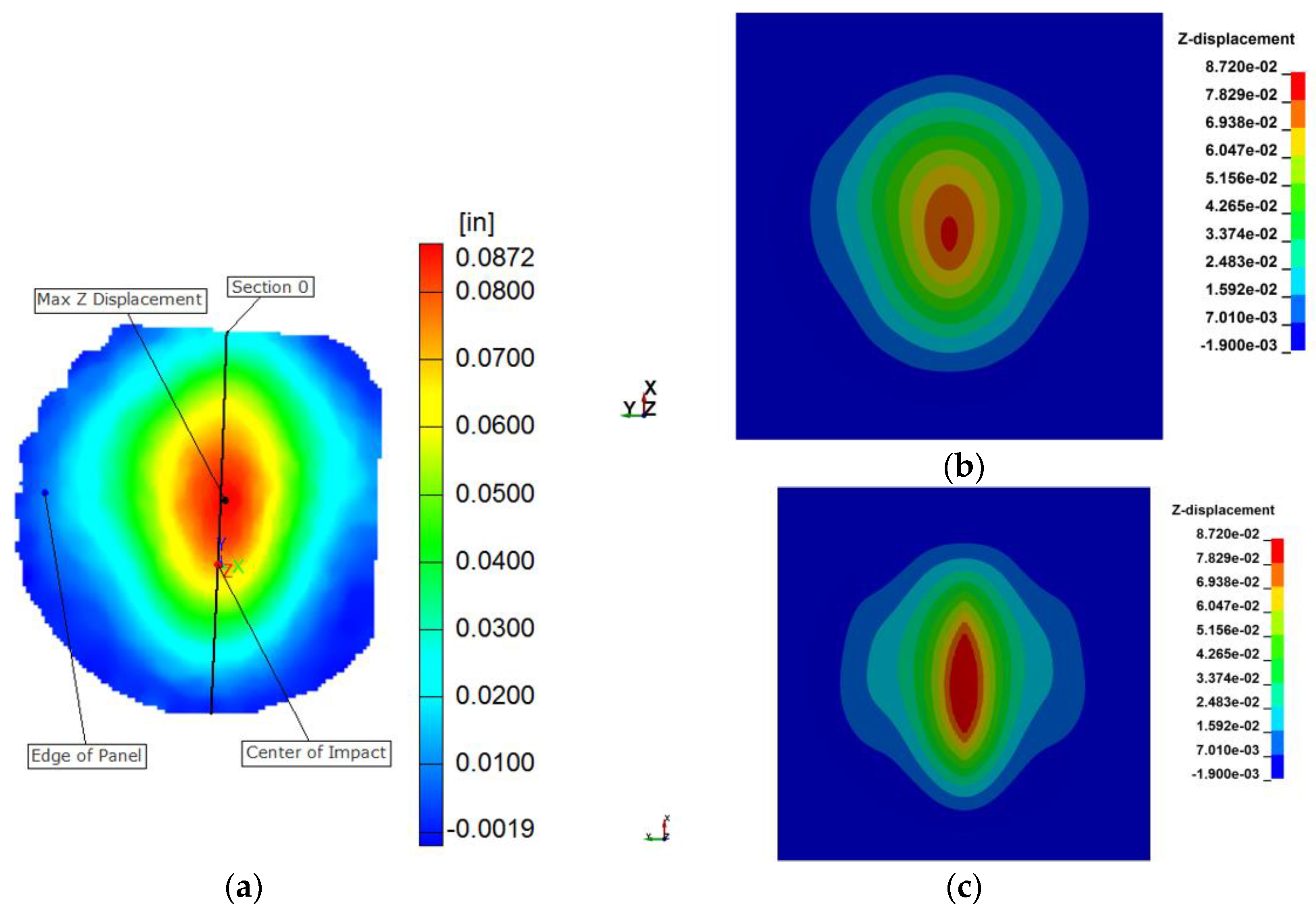
Two comparison metrics were used—the maximum out-of-plane (
Z-direction) displacement and the contour of the out-of-plane displacements, both on the back face of the plate. The contour plots are shown in
Figure 6 for
t = 0.0007 s. The MAT213 results (
Figure 6b) are very similar to that of impact test (
Figure 6a), with a rounded shape that is slightly elongated in the fiber direction especially below the center of impact (COI).
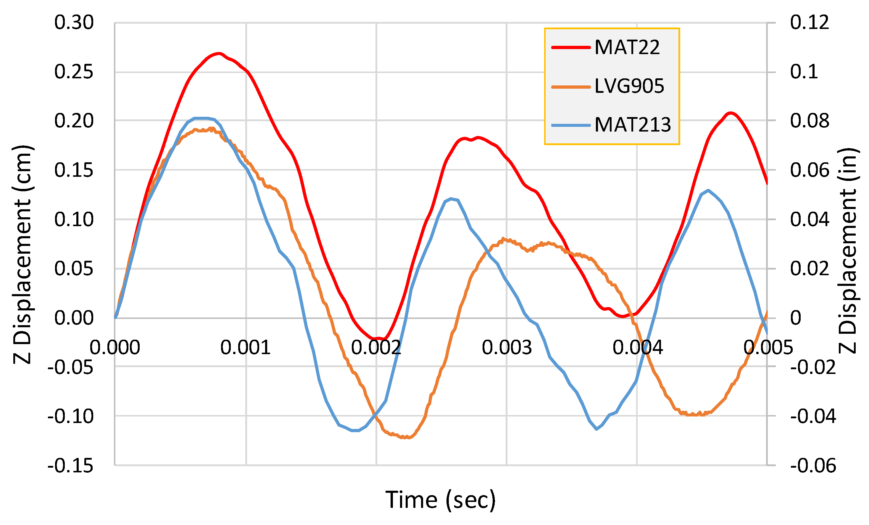
Figure 7 shows the out-of-plane displacement versus time results for the test and the simulations. The results are discussed in the next section.
4. Discussion
MAT213 results show that both the positive peak and the negative peak displacement values are close to the test values for the first cycle (
Figure 7). Thereafter, the peak displacements are overestimated. In addition, there is a difference in the period. Nevertheless, the maximum positive and negative displacements are within a few percent of the experimental values. MAT22, on the other hand, over-predicts the maximum positive displacement (by about 35%) and under-predicts the maximum negative displacement (by about 80%). The displacement contours for MAT213 (
Figure 6b) are very similar to that of the experiment (
Figure 6a)—an ellipsoidal shape with the major axis in the fiber direction. MAT22 (
Figure 6c) shows a more pronounced elongated distribution of displacements in the fiber direction. It should be noted that MAT22 has been developed for use with composites that essentially exhibit linear behavior with sudden, brittle failure.
Finally, it should be noted that there are a few differences between the impact test and finite element models. First, in the impact test, the projectile impact was not a direct hit, i.e., the roll, pitch and yaw angles were not all zero. However, zero roll, pitch and yaw angles were assumed in the finite element models. While the desired center of impact was the center of the panel, due to the low velocity, the center of impact was below the center of the panel (
Figure 6a); second, it is likely that the period differences in the test and FE models are partly due to no damping parameters being used in the FE models.
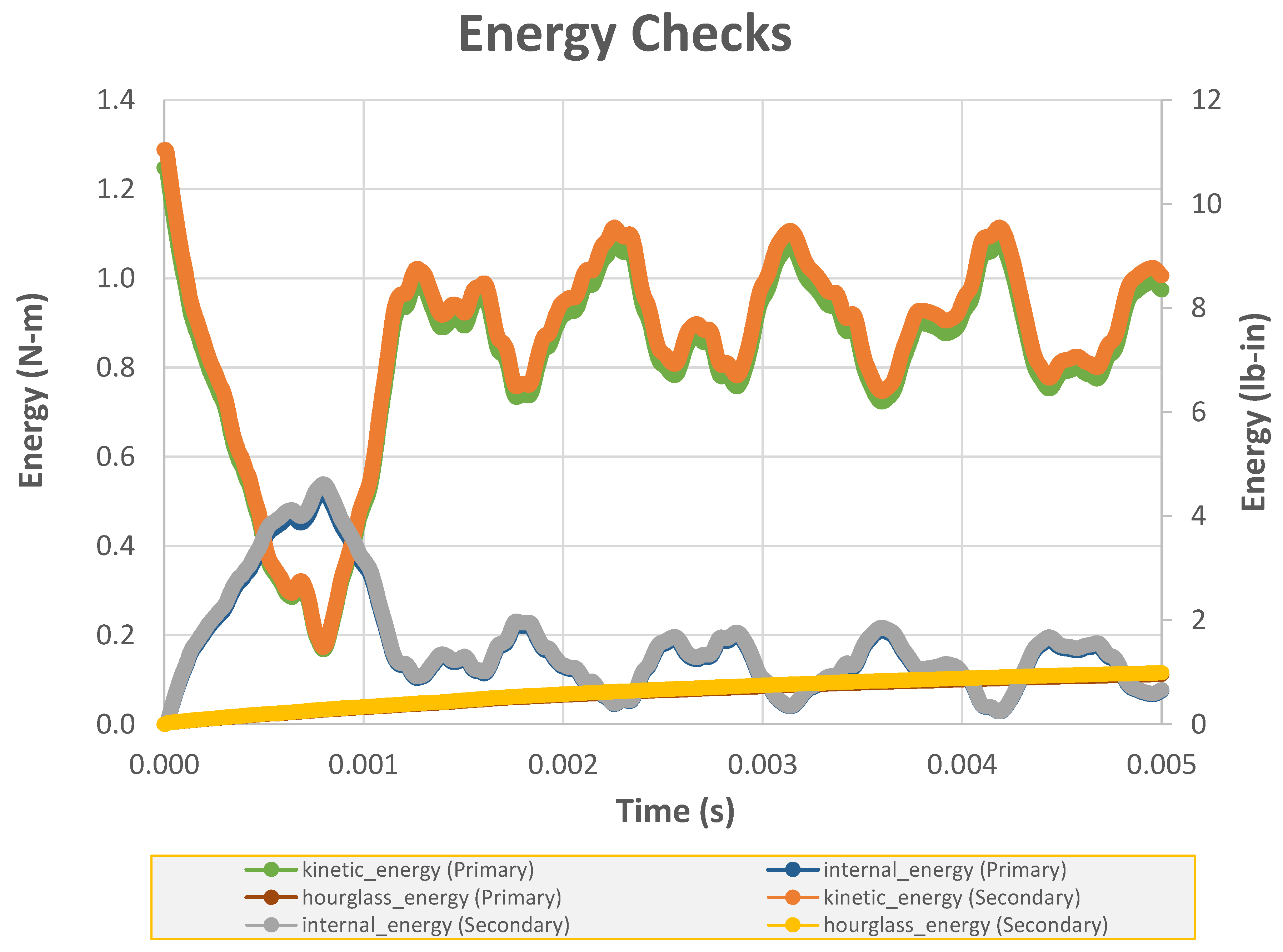
Figure 8 shows the energy checks are used to gage the quality of the finite element solution. The total kinetic energy and the total internal energy appear to vary reasonable well with time. The hourglass energy values are relatively small (less than 10% of the total energy).
The total wall clock time for the MAT213 run was about 13 h and 38 min and for the MAT22 run 2 h and 3 min.
5. Conclusions
A new material model and computational framework have been developed for modeling orthotropic composites subject to impact loads. The algorithm has been implemented in a special version of LS-DYNA as MAT213 material model. The deformation model is driven by a set of 12 tabular data representing stress–strain curves for one temperature and strain rate combination. A semi-coupled, directional-dependent damage tensor is used to capture the effects of damage. The failure model is under development. The behavior of a unidirectional composite, T800/F3900, is used to verify and validate the developed material model. Preliminary results from modeling an impact problem indicate that the implementation is robust and accurate.
Several efforts are underway to improve the material model. First, a failure model is being developed so that element failure can be predicted and if necessary, the element can be eroded from the FE model. This will allow for modeling of a wider array of actual impact tests where deformation, damage and failure take place. Second, the code implementation has not been optimized for speed. It is expected that significant increase in speed would be possible with code optimization (vectorization, loop unrolling etc.). Third, the code has not been validated against impact tests with sufficiently high velocity where rate, and possibly temperature-dependent material behavior, is an important part of the FE behavioral model. While MAT213 has the capabilities to model these scenarios, experimental data is not currently available and the research team is exploring ways to conduct material characterization and impact tests to yield the data.


