A Method for Simplification of Complex Group Causal Loop Diagrams Based on Endogenisation, Encapsulation and Order-Oriented Reduction


Faculty of Informatics and Management, University of Hradec Králové, Rokitanského 62, 50003 Hradec Králové, Czech Republic
Systems 2017, 5(3), 46; https://doi.org/10.3390/systems5030046
Submission received: 12 May 2017
/
Revised: 10 July 2017
/
Accepted: 12 July 2017
/
Published: 14 July 2017
(This article belongs to the Special Issue Systems Approaches and Tools for Managing Complexity)
Abstract
:Growing complexity represents an issue that can be identified in various disciplines. In system dynamics, causal loop diagrams are used for capturing dynamic nature of modelled systems. Increasing complexity of developed diagrams is associated with the tendency to include more variables into a model and thus make it more realistic and improve its value. This is even multiplied during group modelling workshops where several perspectives are articulated, shared and complex diagrams developed. This process easily generates complex diagrams that are difficult or even impossible to be comprehended by individuals. As there is a lack of available methods that would help users to cope with growing complexity, this manuscript suggests an original method. The proposed method systematically helps to simplify the complex causal loop diagrams. It is based on three activities iteratively applied during particular steps: endogenisation, encapsulation and order-oriented reduction. Two case studies are used to explain method details, prove its applicability and highlight added value. Case studies include the simplification of both original group causal loop diagram, and group diagram adapted from a study already published in a prestigious journal. Although the presented method has its own limitations, meaningfulness of its application in practice is verified. The method can help to cope with the complexity in any domain, in which causal loop diagrams are used.
1. Introduction
“Simplicity is complexity resolved.”—Constantin Brancusi
Miller [1] postulated that there is an upper limit of human capacity to process information on simultaneously interacting elements with reliable accuracy and with validity. Other studies from various disciplines [2,3] in which the overall idea and limit of the capacity was scrutinised, investigated or tested have been published since this idea was introduced [4,5]. Saaty [6] (p. 234) states that “the number 7 is perhaps a measure of short term memory capacity for processing cognition and is a different limit than the number 4, perhaps a measure of attentional capacity”. General limitations of human performance are often classed together. These are called as cognitive spans. Such limits are widely known as attention span, memory span, perceptual span, apprehension span, central computing space, channel capacity, or span of absolute judgment. They all represent limits on the amount of sensations, impressions, or distinctions. These that can be held in mind briefly and grasped at once, or used as a foundation for making judgments. The main purpose of this introductory note is to highlight that the limit beyond which human cognition fails, is closer than one could expect. It also means that complex phenomena emerge suddenly and we have to cope with the complexity on daily basis.
At the general level, capturing the concept of complexity is not an easy task as it is multi-perspective in its nature [7,8]. Moreover, there is a plethora of definitions or descriptions available. For instance, one of the existing approaches to complexity in biology is grounded in an idea that physical complexity, as a measure based on automata theory and information theory, is a simple and intuitive measure of the amount of information that an organism stores in its genome, about the environment in which it evolves. It is argued that physical complexity must grow in molecular evolution of asexual organisms in a single niche if the environment does not change, due to natural selection [9]. A technical definition of complexity involves the quantity called algorithmic information content. The description of an entity is converted to a bit string and a standard universal computer is programmed to print out that string and then halt. The length of the shortest programme (or, respectively, the shortest that executes within a given time) is the algorithmic information content [7]. Furthermore, sub-concepts can be found in the literature, where structural complexity or time complexity are studied and applied in research. For instance, time complexity, expressed typically in the “big O notation”, is a concept used in computer science. It deals with the quantification of the amount of time taken by a set of code or algorithm to process or run as a function of the amount of an input. Similar to the complexity definition, it is quite difficult to identify a general approach for reduction of system complexity. It is due to the strong dependency of complexity reduction and the discipline, in which this process is conducted. Methods or techniques differ significantly in particular areas, for instance in computer science [10], hydrology [11] or health care [12]. Due to this issue, general point of view on complexity as a function of amount of system elements and their mutual interrelationships is applied in this study.
Systems thinking can help stakeholders better understand how complex interconnections of multi-level factors influence various phenomena in a plethora of disciplines such as evaluation [13], prevention science [14], public health [15], urban planning [16], or business administration [17]. Systems thinking helps practitioners understand system complexity and bear it in mind, which is necessary to overcome natural human tendency to apply mechanistic approach built on cause-and-effect and linearization principles [18] and thus miss “unintended” consequences of actions (e.g., intervention and policy change) that undermine the effort over time [19]. The application of systems thinking leads to the development of comprehensive models. Furthermore, complex problems produce complex models that are difficult to be understood. If dynamics is included, the comprehensibility even decreases [20]. The problem is that dynamic systems surround us, and can be identified everywhere. As time goes by, static systems represent only snapshots of dynamic behaviours of systems-of-interest. The complexity of dynamic systems is rooted in many system attributes ranging from nonlinearity to relationships between multiple causes and their effects [21].
Endeavours to cope with the dynamics and complexity in a systemic way are based on various tools, methods or techniques. Among the numerous approaches available to understand complexity [22], systems science methods appear the most promising [23]. Bayesian networks, agent- or knowledge-based models, and system dynamics tools can serve as examples [24]. Each of these systems thinking methods provides unique strengths and helps stakeholders to explore systemic problems in different but complementary ways. Bayesian networks are grounded on the probabilistic approach to description of the connections among system variables [25]. Agent-based models deal with agents of different types that are characterised by certain behaviour. In fact, agent-based modelling complexity represent the main advantage as models of systems with thousands specialised agents are developed and system behaviour is simulated. Agents represent system’s building blocks and their combination brings synergic effects and emergent properties [26]. Systems science simulation modelling approaches, such as Agent-Based Modelling, have been used to quantify diagrammed relationships, inform about evaluation targets, or compare intervention effects [27]. In knowledge-based systems knowledge is stored in a knowledge base and then an inference mechanism is applied to infer conclusions. In this way, the complexity embedded in a problem is resolved by a machine. Additionally, the cognitive limitations of people are overcome [28].
The remainder of the paper is structured as follows. After the short introduction to complexity in this section, the main research problem is formulated in Section 2. Section 3 provides the explanation of the proposed method and explains its assumptions and particular steps. Section 4 comprises two case studies that are used for the demonstration. Consequently, study limitations and further research directions are outlined. The final section concludes the paper.
2. Problem Definition
The last discipline not exemplified in the Introduction Section represents the main field of study and context in which this paper is created. System dynamics deals with understanding how the system behaviour changes over time and is gaining popularity due to its flexibility and structural focus [29]. It has already been applied with the intention to support decision-making in many disciplines ranging from chronic disease risks [30] to urban coastal systems [31]. The underlying premise of the approach is that the dynamic behaviour of complex systems is a consequence of system structure [24]. Building models helps to understand the feedback loops, delays, nonlinearities, or accumulation of variables that all together express the relationships among system components [32]. There are two sides to the modelling process in system dynamics which support each other [29]. First, the process deals with the mental models of users, stakeholders or experts and elicits the causal assumptions about the system. Consequently, created models test the validity of these assumptions. Second, all users are considered as an essential part of the modelling process which supports openness, diversity and self-reflection. The outcome of the modelling process can have a form of diagrams, mostly stock-and-flow diagrams, or causal loop diagrams. As the former diagram type enables quantitative simulation, the latter offers visual grounded logic models and represents the main topic of this study. The causal loop diagrams provide a method to map the complexity of a system of interest that comprises variables, causal relationships and polarities of both links, and feedback cycles [33].
It is reported [34] that spread of causal loop diagrams as a tool for modelling system dynamics was strongly supported by Goodman’s study [35], in which diagramming process is explained together with details such as loop polarity determination.
There are various issues associated with the syntax and practical application of the causal loop diagrams. For instance, to depict problems with softness and inconsistency, Richardson [36] suggests the following experiment: “take the causal-loop diagram of the family feud and ask a random sample of system dynamics modellers or students how it will behave. In my experience, one will not only receive a wide range of answers but most of these will be incorrect”. He focuses also on other problems and summarises them in his seminal work. There he deals with definitions of positive and negative feedbacks that represent building blocks of causal loop diagrams and associated problems with common definitions, rate-to-level links, hidden loops, or net rates. He for example provides modified link definition that helps to cope with problems of influence directions indicated by arrows (links) in diagrams. Another guru of system dynamics modelling, John D.W. Morecroft, critically reviews diagramming tools used for conceptualising feedback system model. He lists causal loop diagram-related weak points such as little correspondence between mental model and loop structure, low reliability of loop structure as a guide to behaviour, possible ambiguity in loop polarity definition, no discrimination of the elements of structure, or that published diagrams belie the original conceptualisation process [34]. Thus, various problems have already been pointed out and solved in the past. However, all described issues call for more research into how causal loop diagrams can be created, interpreted and used in practice.
The main issue that represents the subject of interest of this manuscript is based on many years of system dynamics practice. In order to avoid the common “the model is unrealistically simple” type of criticism, modellers are tempted to build large and too detailed models, which often makes the situation even worse since the final product is large and too complicated but still unrealistic [37]. It is related to natural tendency of users to develop more complex models in order to capture all relevant variables and explain more phenomena included in the problem situation. Here the main problem arises. Modelling of causal loop diagrams mostly focuses on development of more complex diagrams in order to acquire more robust perspective on particular phenomenon. The development of group-based diagram described in the next section can serve as a good example of this practice. The growing complexity is considered as natural trait that individuals have to reconcile with. The related reduced comprehensibility of the acquired models remains mostly unsolved. As a result, complicated outcomes which individuals with limited cognitive skills cannot understand are presented. Then, due to estimate cognitive limits [6], only model fragments are taken into consideration and the value of the acquired complexity in the causal loop diagram diminishes. Richardson [36] states that “there is a natural human tendency, it seems, to be more consistent than accurate when one can’t be both”. Unfortunately, with complex models at hand, it seems that their users cannot be both. Sterman [38] discusses the appropriate model boundary and level of aggregation in system dynamics models to demonstrate that larger or more disaggregated models are appropriate in some circumstances. However, for many problems a small model is sufficient to explain problem dynamics and build intuition regarding appropriate responses [39]. The complexity of a causal loop diagram can be expressed in many ways. For instance, McGlashan et al. [21] apply indicators used in the network analysis domain. They describe their diagrams by metrics such as the average path length in the network (in how many causal paths variables are able to reach each other on average); the most distant variables (identification of the shortest path between variable), which determines the CLD’s diameter; or the network modularity that indicates the presence of structural clusters of variables in the network.
Barlas suggests that there must be an additional final step in system dynamics modelling, namely model simplification, which completes the modelling cycle with a much simpler, fundamental version of the working model [37]. While various disciplines deal with investigating possible ways how to improve readability of visual system representations, e.g., edges bundling [40] or network folding [41], the complexity simplification does not belong to the mainstream extensive research areas in system dynamics and it is mostly out of scope of practitioners. System dynamists mostly focus on quantitative analysis of existing models (eigenvalue, elasticity, feedback dominance, etc.), which is however associated with quantitative modelling only. In fact, only few studies published in prestigious resources focused on various aspects of system dynamics has been identified from 9850 records in the System Dynamics Bibliography. Consequent search in Scopus and Web of Science databases did not provide any other relevant record. Only three of them are exemplified in this section, where representatives of formal mathematical, qualitative and quantitative modelling are stated. At the end of the 1980s, Eberlein [42] presented a formal theory of model simplification as a means of increasing model understanding, which identifies important feedback loops in linearized models with respect to a selected dynamic behaviour. Frannek et al. [43] introduce the simplification method based on node importance and centrality as inputs into the process of nodes consolidation. Authors demonstrate method’s usability on the case of department store visitor prediction. Saysel and Barlas [37] present their approach to simplification which is based on performance of five main steps: identification of the reference behaviour, selection of sectors with weak feedback relations, selection of parameters candidates for aggregation, flow simplification, stock-flow simplification and iteration of the procedure unless the established criterion is broken. In addition to introduced methods, other trivial techniques such as colouring [44] or burdening thematically oriented substructures [45] are applied occasionally. However, in really complex diagrams, these help only to split the content with the complexity almost unsolved. This represents the main research gap that this manuscript aims at. The main objective of this study is to present a novel method for systematic simplification of causal loop diagrams complexity.
3. Method Description
There are several assumptions associated with the method. First, as system dynamics is based on system-as-a-cause thinking [18], the system structure ought to fully explain system behaviour. Second, the method expects no discussions about the suitability of reduction the model by any variable. During the model building, the complexity together with the information value is increasing. We have to bear in minds that the opposite process brings the opposite result—a loss of the information value with decreased complexity as a benefit. The model is a simplified version of reality; hence, something is always missing. This is exactly why the simplification process takes place. Third, the whole picture is more important than the detail. The opposite interpretation of the “the devil is in the detail” phrase known for system analysis [46] can be applied here. Although important, details make things more complicated and provide limited contribution to the insight into the problem and a big picture needs to be preferred. Last, multi-input and multi-output (MIMO) variables are those which shape the system structure and significantly influence system behaviour. Thus, the reduction needs to be performed from the simplest model elements (pure inputs, sometimes denoted as out-degrees, and outputs, sometimes detonated as in-degrees [21]) to more complicated single-input single-output (SISO) variables, single-input double-output and double-input single-output (SIDO and DISO, respectively) variables, double-input double-output (DIDO) variables, etc. Apparently, as the complexity grows, proportionally the order of variables included in the model does. Thus, although it may seem that removal of for instance DIDO variables can have a drastic impact on the model value, the opposite is true. The level of relative reduction (whole system complexity vs. the highest order of removed variables) is quite similar at all levels of the complexity.
The introduced method is grounded in three main activities: endogenisation, encapsulation, and order-oriented reduction. In fact, the method as a whole is centrality-oriented as it primarily supports MIMO variables while in-degree, out-degree, and betweenness (mediator) variables are suppressed [21]. Three activities presented above are ordered here according to extent of their damage on systemic nature of described model caused by the simplification. Therefore, the sequence in which they are conducted should respect this trait. If endogenisation can be done, it needs to be preferred to encapsulation. If encapsulation can be performed, it has to be applied instead of reduction. The following sequence of steps ensures proper implementation of the method. As the complexity can be tamed mostly in an iterative way [47] the method is iterative in its nature and several repetitions have to be done with respect to the complexity/simplicity ratio of the causal loop diagram.
Sequence
- (1)
- Construct a diagram and use duplicate variables (ghosts) only as inputs to other variables—as the complex diagram contains tens of even more variables, it is not possible to draw it without crossing single links. The readability of the diagram is usually improved by usage of duplicates or so called “ghosts”. If these are applied, they should be used merely as inputs. It improves the orientation in the complexity at the beginning of the process. As variables are replaced or removed, the amount of ghosts is reduced as well.
- (2)
- Define required complexity of the model—the complexity can be defined in various ways. The casual loop diagrams are mostly developed in the graphical form and are complex. Therefore, it is almost impossible to find all paths in the model. Moreover, this does not represent the most appropriate criterion for final complexity setting. Pragmatically, one can use number of variables or better an interval in which the final number of variables will occur.
- (3)
- List all exogenous variables, i.e., model inputs and outputs—exogenous variables usually represent quite significant portion of model variables (see case studies below). They need to be listed due to valuable information that will be lost during the simplification procedure. It can be used later for better understanding of the simplified model.
- (4)
- Mark inputs and outputs and associated blind branches—all exogenous variables have to be marked before their exclusion. It is recommended to remove all variables in one step to avoid disorientation caused by the occurrence of new exogenous variable that may be created as a result of this step. Blind branches help to speed up this step as well. Blind branches are represented by cause-and-effect relationship among exogenous variables (leaf of the branch) and other consequent variables without feedbacks. Every blind branch end in a variable which is a part of any feedback loop.
- (5)
- Erase selected variables (endogenisation).
- (6)
- Mark SISO variables—when exogenous variables are removed, the system behaviour is completely explained by its structure. SISO variables represent only transformation elements that help to get the system dynamics from one point to another without any contribution, or better to say with contribution that can be substituted by a structural change. Again, it is recommended to mark all SISO variables and remove them simultaneously.
- 7)
- Bridge SISO variables (encapsulation)—during this step, there are two issues that need to be considered. First, it is necessary to define polarity of a new link. For these purposes, the same principle used for definition of the feedback loop polarity can be used [38]. The new polarity can be determined based on number of links with negative polarities. The SIGNUM function is used for this purpose, as it returns two values only—0 or 1—which clearly define the link polarity. Second, this procedure results in elimination of simple local feedback in which only two variables are included. However, this is in concordance with the assumption about preference of the global picture to details.
- (8)
- Perform Steps 2–5 unless the model is fully endogenous again—in the following Steps 8–10, the main aforementioned principle is applied. After the removal of local feedbacks, new exogenous variables may appear.
- (9)
- Perform Steps 6–7 unless the model has no SISO variables again.
- (10)
- Repeat Steps 8–9 unless all exogenous variables and SISO variables disappear.
- (11)
- Mark all SIDO and DISO variables
- (12)
- Erase SIDO and DISO variables (order-oriented reduction)
- (13)
- Perform Steps 2–5 unless the model is fully endogenous again.
- (14)
- Perform Steps 6–7 unless the model is fully endogenous again.
- (15)
- Repeat Steps 8–9 unless all exogenous variables and SISO variables disappear.
- (16)
- Repeat Steps 11–15 with DIDO variables, triple variables (SITO, TISO, and TITO), etc., unless the required complexity is obtained.
The procedure may seem to be very long for the application in practice. It is caused by the embedded iterations. Nevertheless, the simplification of the majority of the diagrams reviewed in the scientific literature can be finished quite soon (see reference in the Introduction Section and case studies below).
4. Results
The method presented in the previous section can be employed for simplification of any complex causal loop diagram. This section demonstrates the method applicability and verifies it with the help of two case studies. Group (or collective) causal loop diagrams created in order to overcome limited cognitive abilities of individuals and to get more complex view on the phenomenon are used in this section. The development of group causal loop diagrams has become widely applied in many domains [48] and has been investigated since the mid 1990s [49,50]. The business administration domain can serve as an example, in which the need for group decision making arises due to the limited perspective, knowledge, or information processing capacity of individuals [51]. This process is quite challenging, but there is a plethora of model-based group approaches developed within the single systems disciplines [52]. Group modelling has its own limitations that have been presented in many studies (e.g., [53,54,55]). However, it represents a good source of complex diagrams that can be used for the purpose of this study. Mostly, the final product of the group diagram development is a complex model with many variables and even more links included (see [56,57]). The main reason for this is grounded in methods applied for grouping together single diagrams [58].
The first case study depicts application of the introduced method in the whole process of group causal loop diagram development in order to demonstrate increase of complexity and its consequent simplification. The intention is to verify if the outcomes from the method are acceptable for those, who developed their own diagrams based on their own mental models. The case study has a form of qualitative research, in which usability is tested with the help of selected subjects. Therefore, rather than quantitative data, insights together with opinions and specific perspectives were gathered. After the application of the method all subject expressed their point of view on the acquired result. The second case study applies the method on the existing outcome available in the prestigious scientific journal. Due to complexity of diagrams and necessity to ensure their legibility, polarity of links is depicted not only by the +/− notation, but also by solid line for the negative polarity (−), and dashed line for the positive polarity (+) in both case studies.
It is important to note that, due to the demonstration purpose, the complexity is not determined in both case studies and both causal loop diagrams are simplified by execution of first 15 steps outlined in the previous section. The rationale is to enable the comparison of final version of simplified diagrams in two distinctive instances rather than to obtain the required complexity. This approach enables to depict which level of simplification can be considered as sufficient or whether too much simplification was conducted. The required complexity is always purpose-specific and depends on tasks that are supposed to be done with the simplified diagram.
4.1. Case Study 1
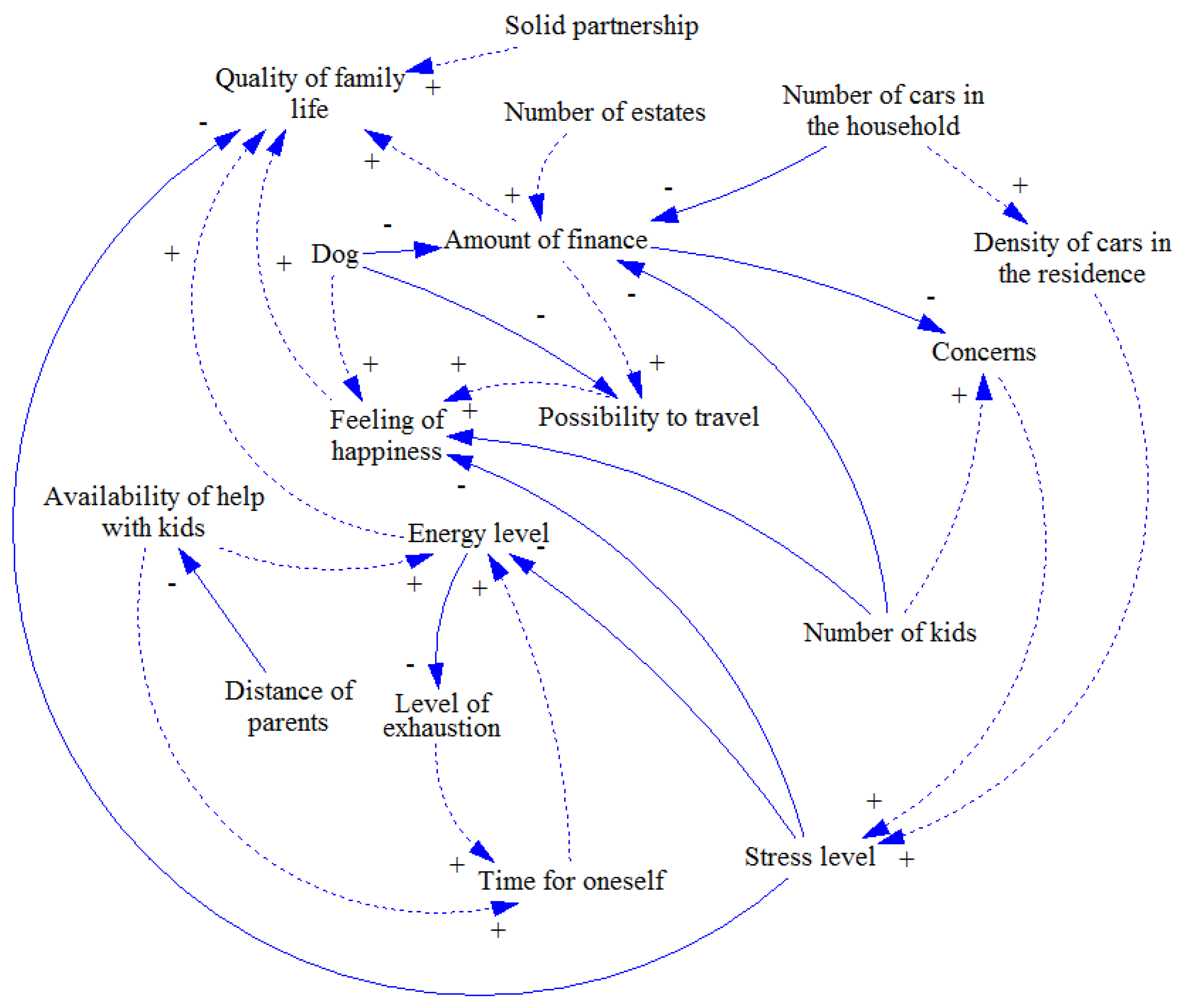
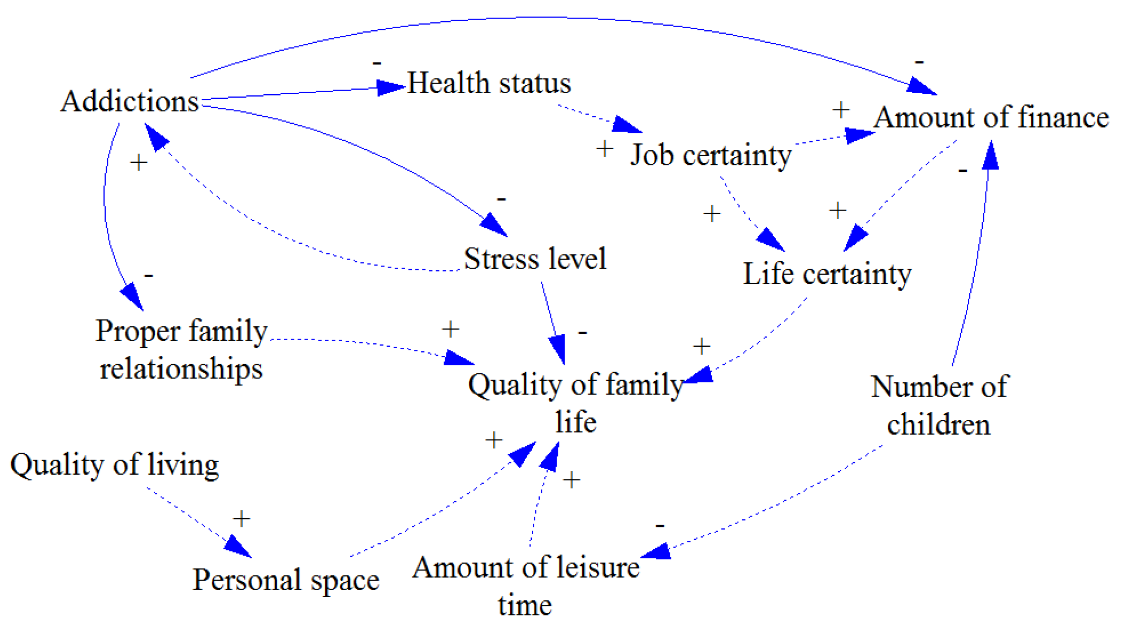
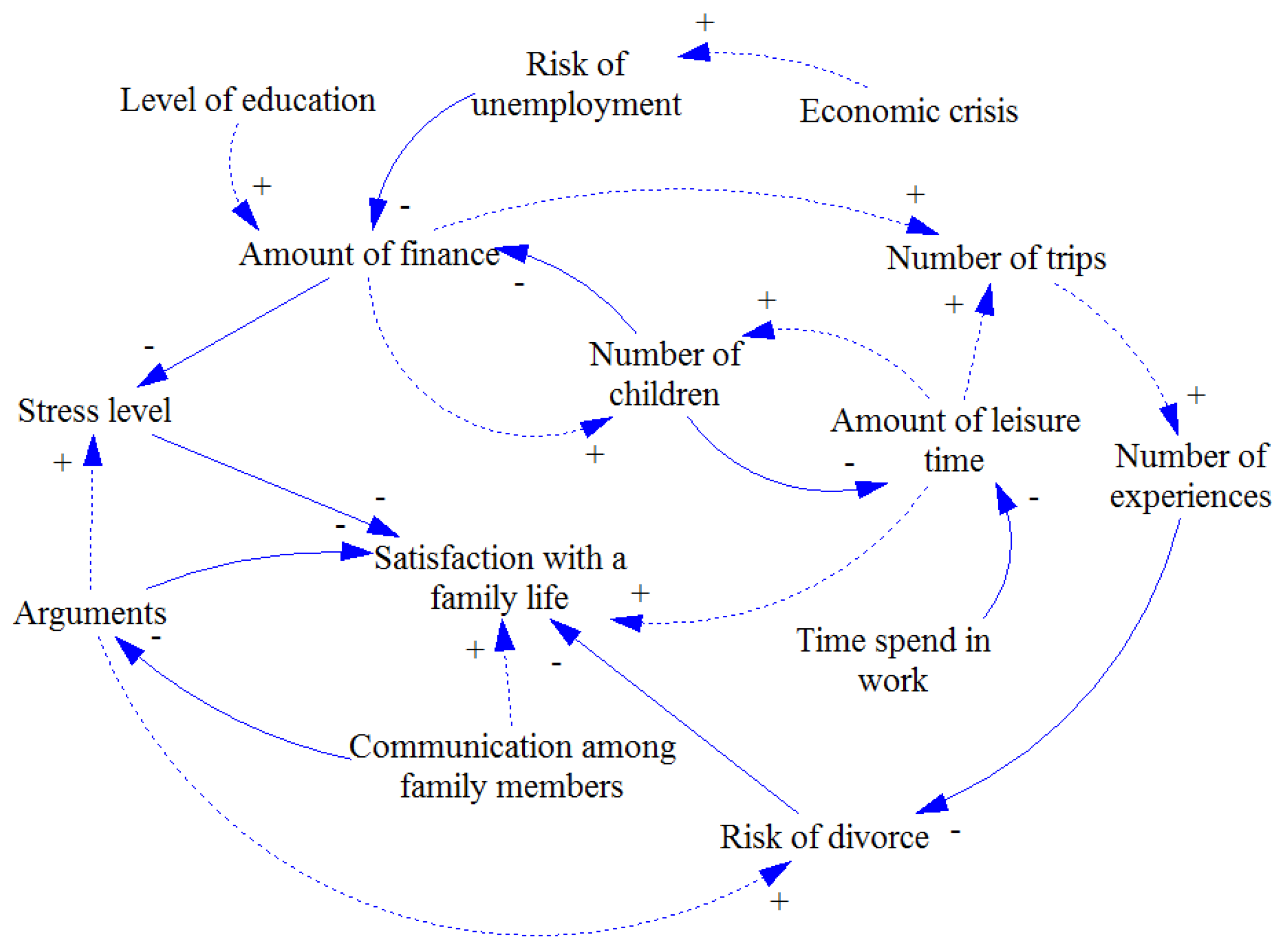
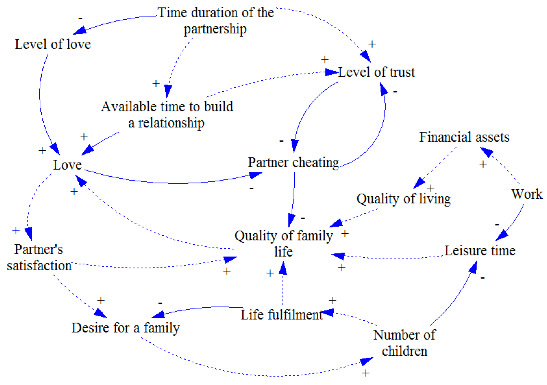
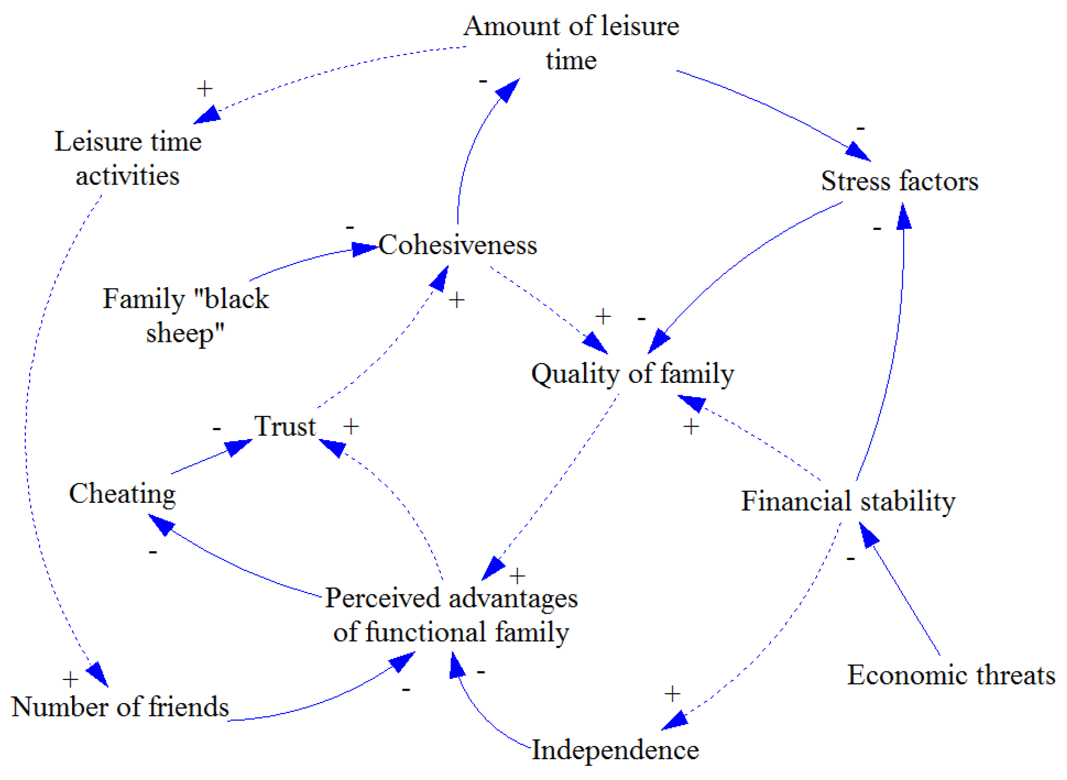
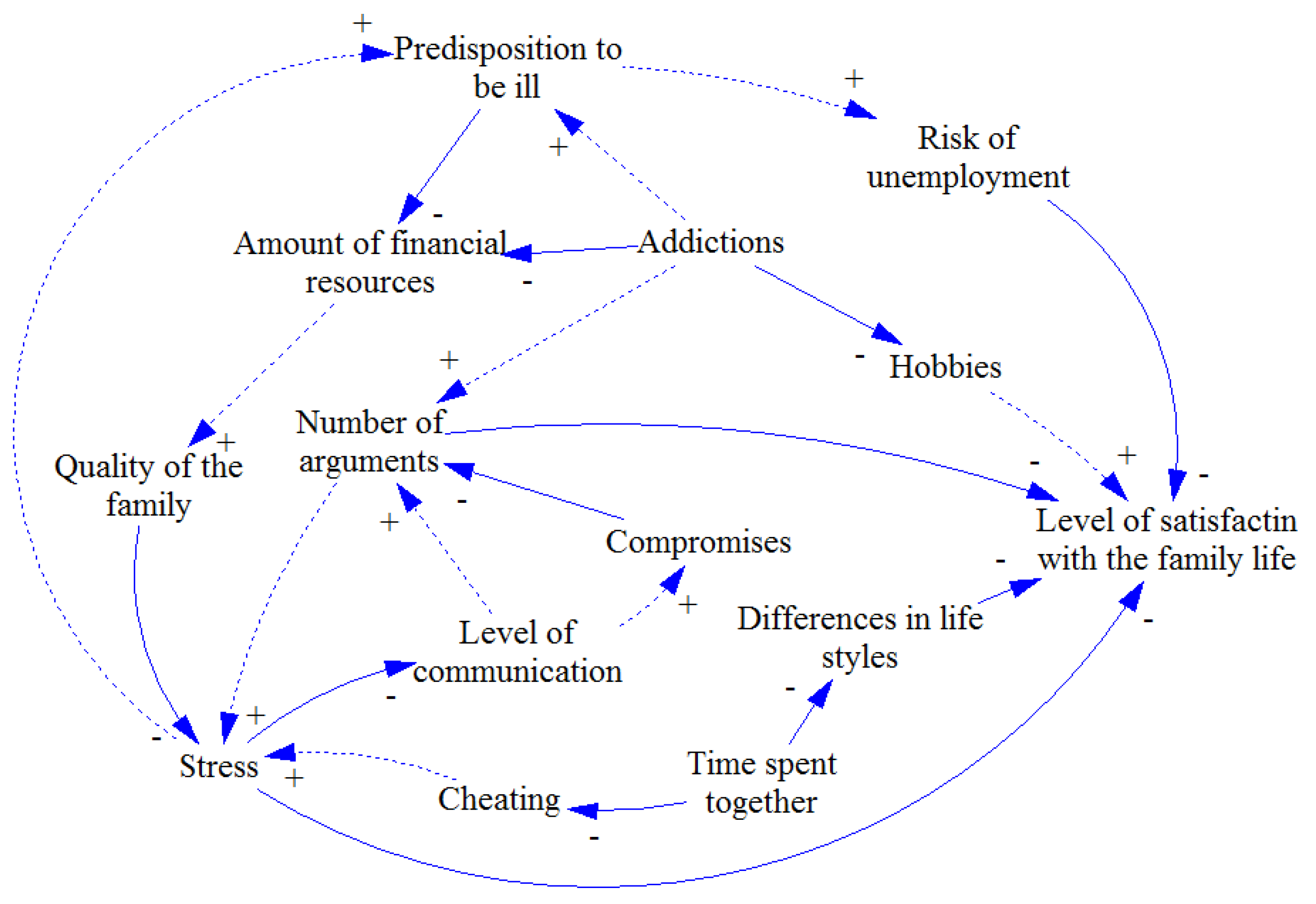
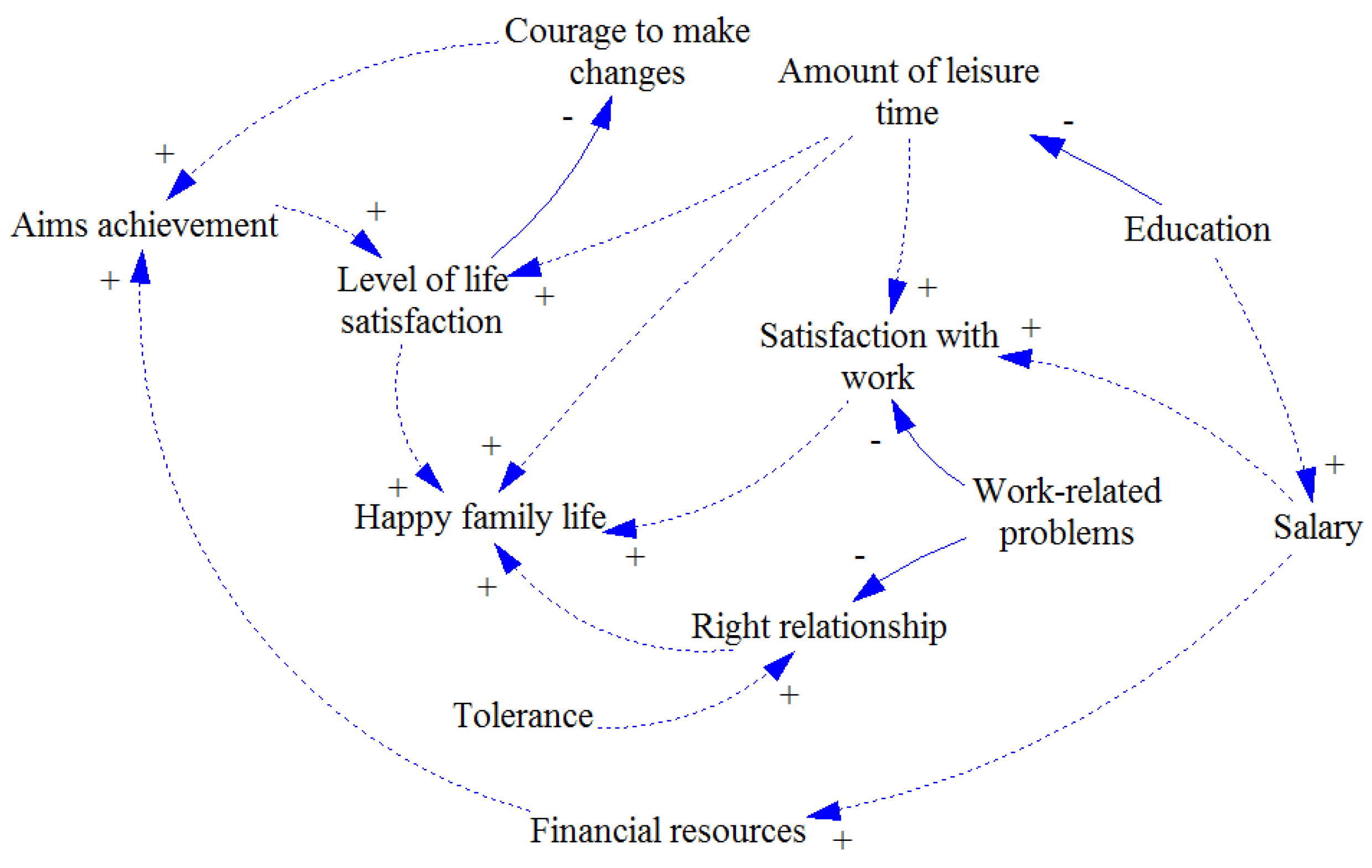
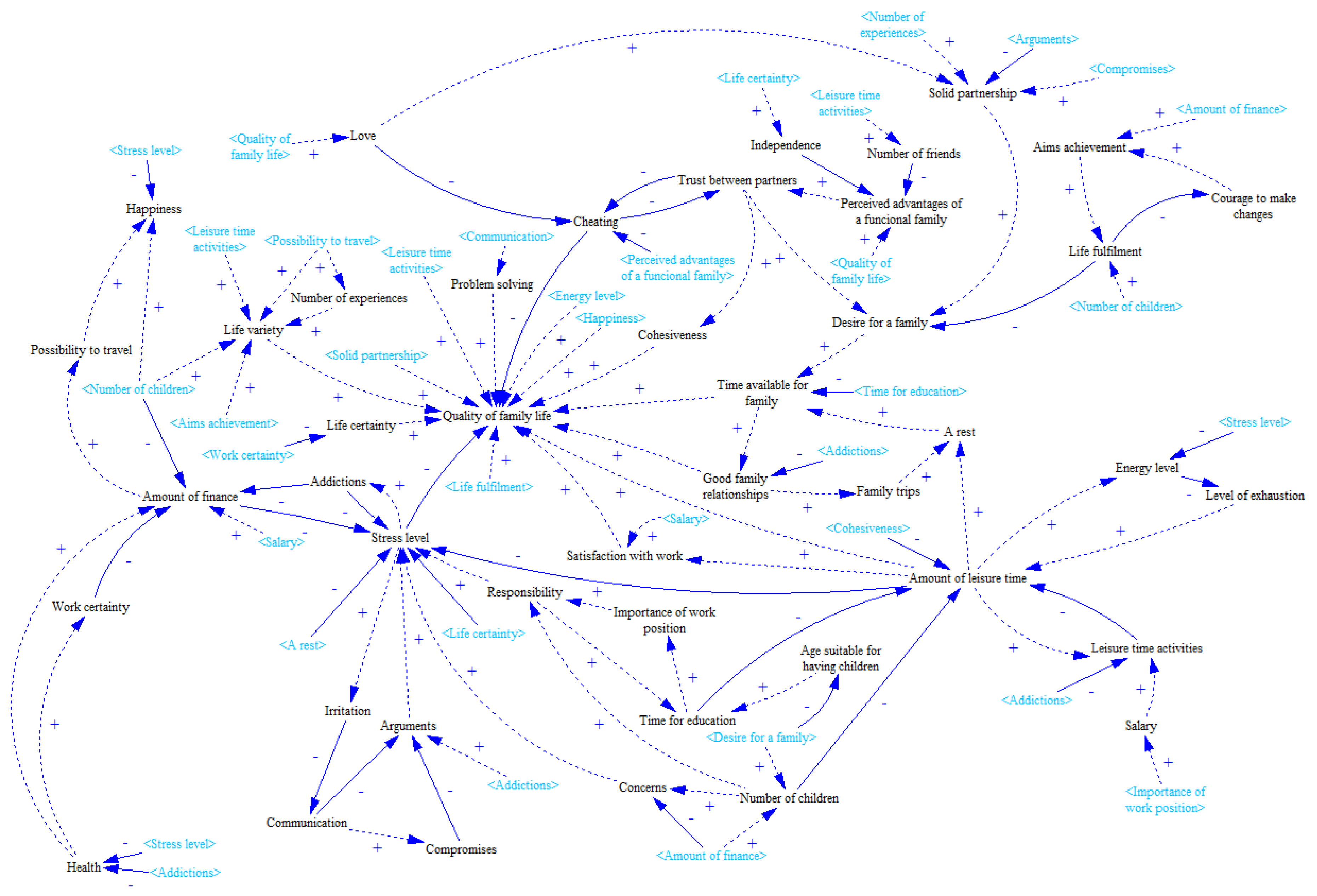
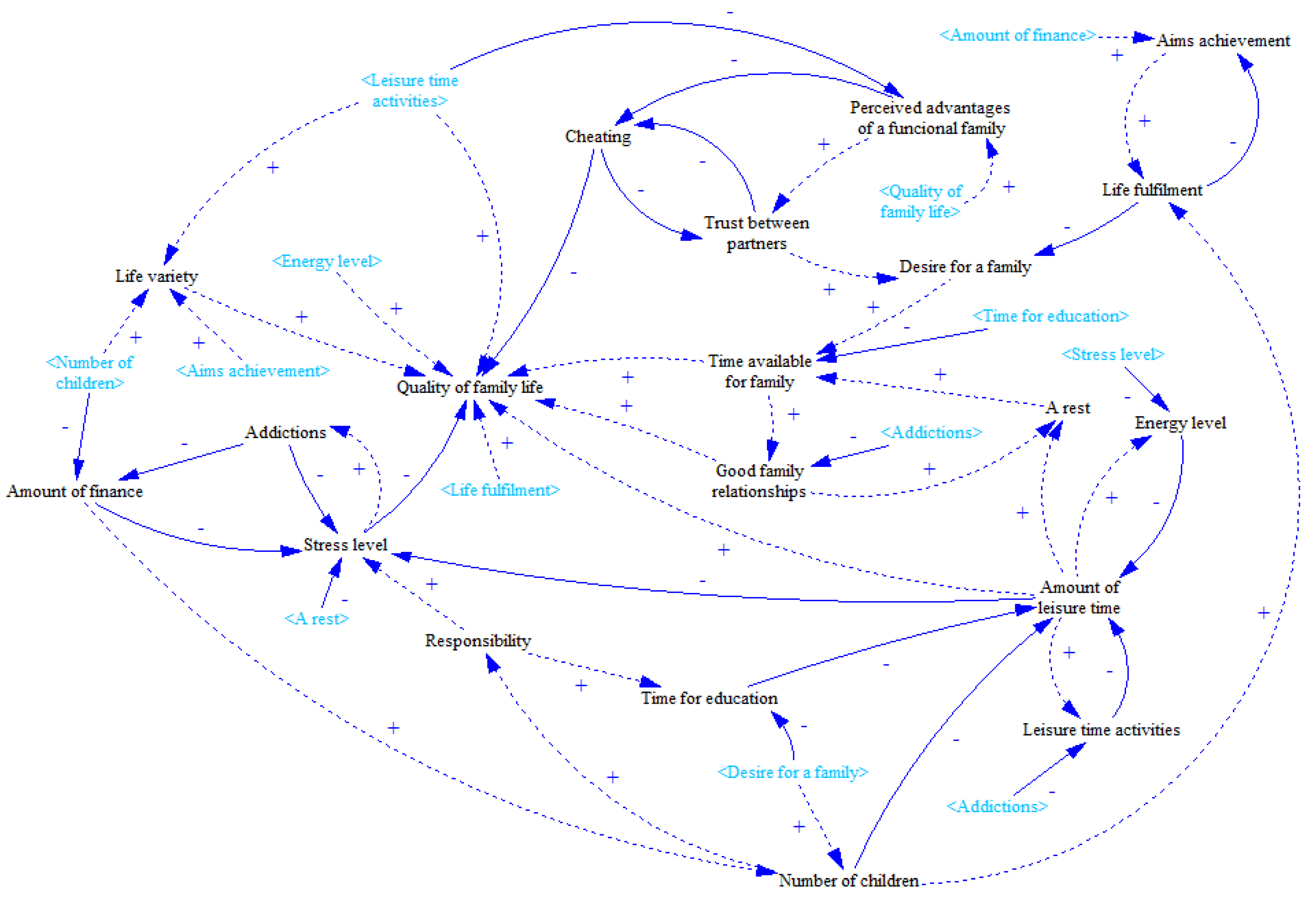
Inspired by the Richardson’s suggested experiment described in Section 2, the first study focuses on family life and related sources of problems or happiness. A sample of ten individuals was acquired by the criteria-based technique. They were not familiar with causal loop diagrams and related syntax. All of them underwent 15 min long introduction after which all agreed to be able to develop simple diagram. There were no limitations to development procedure or diagram size to get true point of view on the topic. The obtained diagrams (see Figure 1, Figure 2, Figure 3, Figure 4, Figure 5, Figure 6, Figure 7, Figure 8, Figure 9 and Figure 10) were consequently redrawn in the Vensim software package, version PLE, which is used for modelling and simulation of system dynamics. Although there were no limits set, the individual diagrams are quite comprehensible due to their low complexity. Apparently, the cognitive limitations of all individuals prevented developing a diagram that would be out of the cognitive span of each creator. In order to take a more complex view, individual diagrams were merged with the help of available methods described in [58]. This procedure resulted in the complex group causal loop diagram presented in Figure 11. As the merging procedure does not represent a subject of interest of this study, the related details such as the compliance of the group diagram with individual diagrams or the identification of shared topics are not analysed.
With the group causal loop diagram at hand, the simplification procedure can begin. The first step is already conducted as the diagram has applied ghosts. Nevertheless, the readability of the diagram due to link crossing is not significantly decreased. As stated in the second paragraph of this section, the Step 2 is skipped. Following the method procedure, all inputs and outputs should be listed. Although this list represents one of two method’s outcomes, it is not necessary to provide it at this place. The simplification method is demonstrated in this study and there is no need to analyse the topic depicted in the causal loop diagram. After marking all exogenous variables (Step 4), they are all erased to make the diagram fully endogenous (Step 5). The outcome acquired from the first five steps is depicted in Figure 12. Consequently, several iterations of first steps need to be done to move further from the endogenisation to encapsulation activity. The examples of partial outcomes are presented in Figure 13 and Figure 14.
Even though it is not possible to determine which extent of the diagram is the most appropriate (diagram can be always extended by other variables or simplified to increase its comprehensibility), the diagram presented in Figure 15 is considered as the final version for Case Study 1, although further simplification is apparently possible. The Quality of Family Life represents the main in-degree variable. Other significant variables are Stress Level, Perception of Advantages of Functional Family, or Amount of Leisure Time. Several both local and more complex feedback loops can be identified. Stress level-related or leisure time-oriented balancing feedbacks represent the local loops. Furthermore, complex reinforcing feedback depicting how Quality of life, Perceived advantages of a functional family, Trust between partners, Desire for a family, and Time available for family influence the overall quality of life can be exemplified. It can be seen that its content is quite similar to content of individual diagrams with slightly higher complexity. It is still the product of group thinking based on single perspectives of ten people. The final version of the simplified diagram was introduced to all ten modellers and they were asked to determine a level of satisfaction or concordance with their point of view. All ten individuals found the simplified diagram as an appropriate representation of the system acceptable from their perspective. The remaining MIMO variables represent the key concepts that have to be, together with list of initial inputs and outputs, considered when thinking about family life-related issues. This verification supports applicability and usability of the method in practice.
4.2. Case Study 2
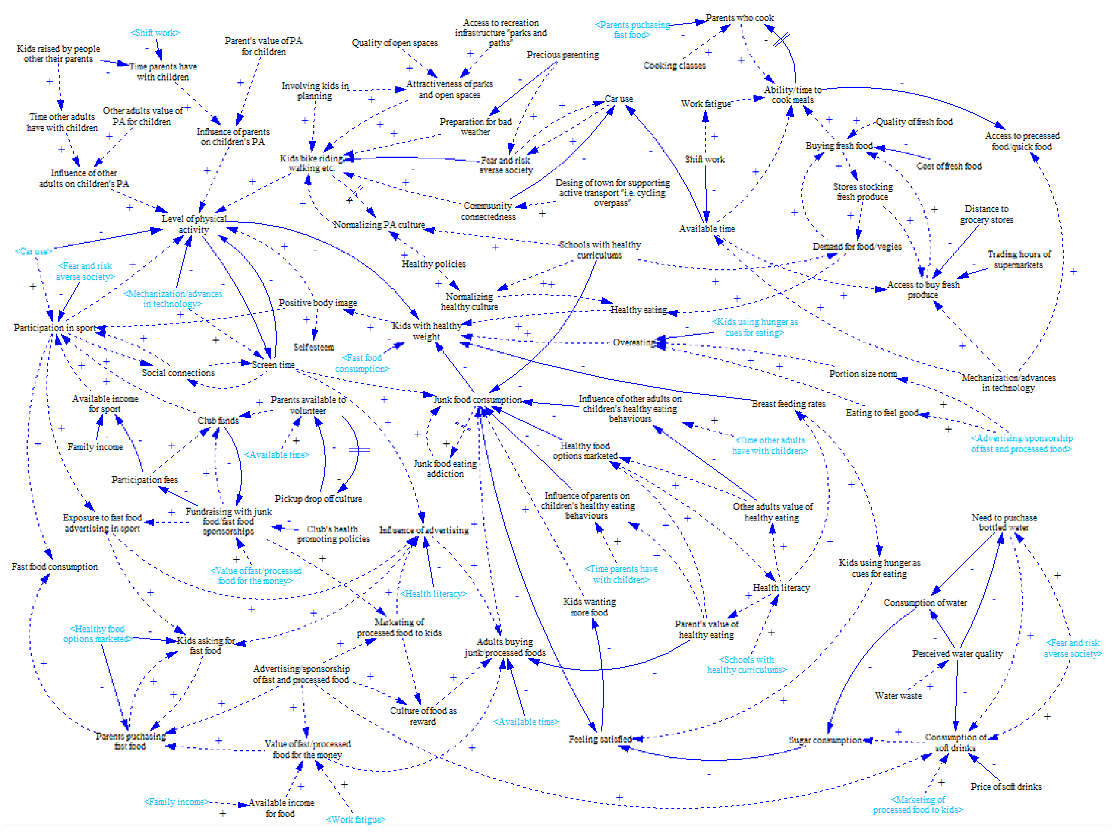
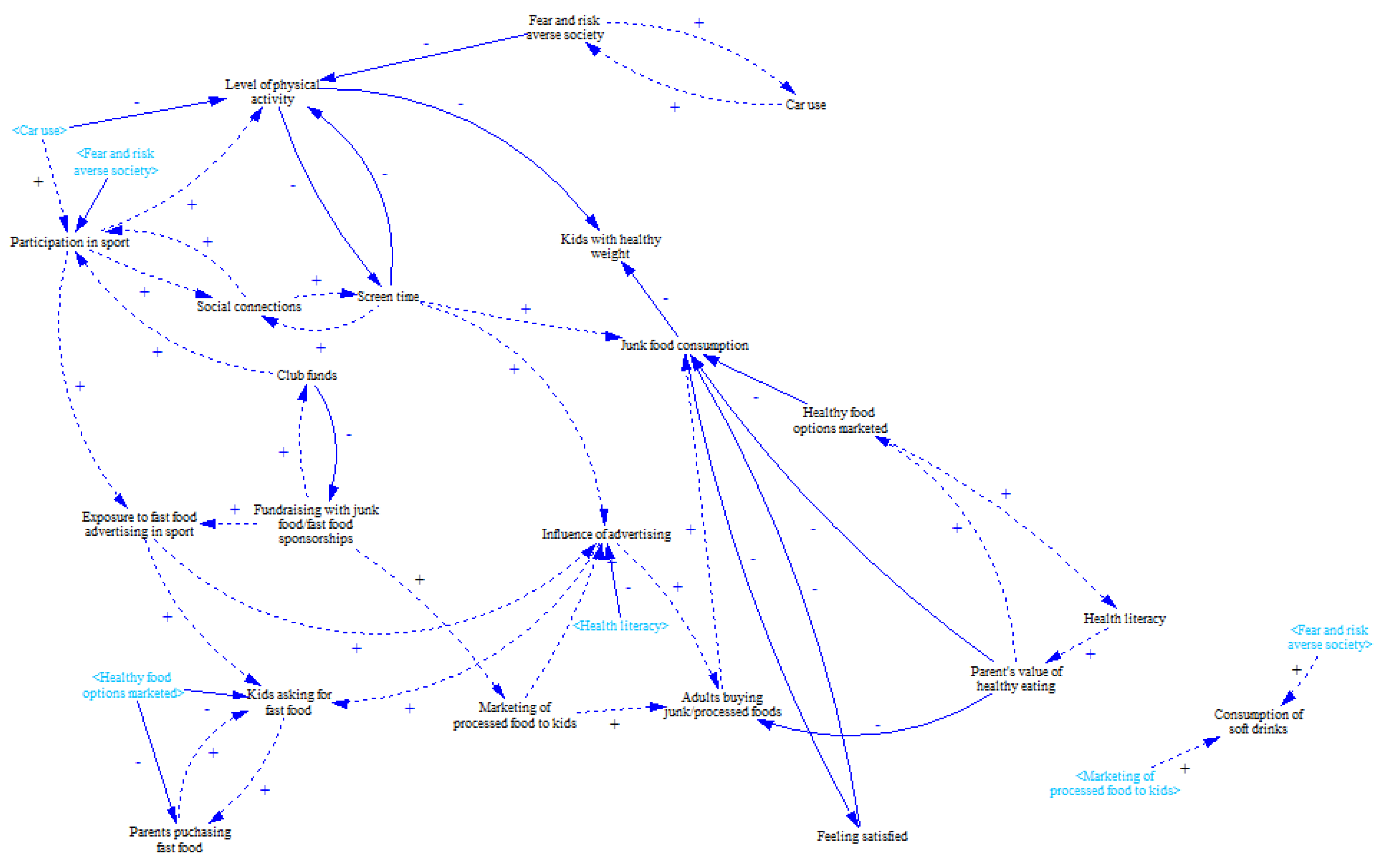
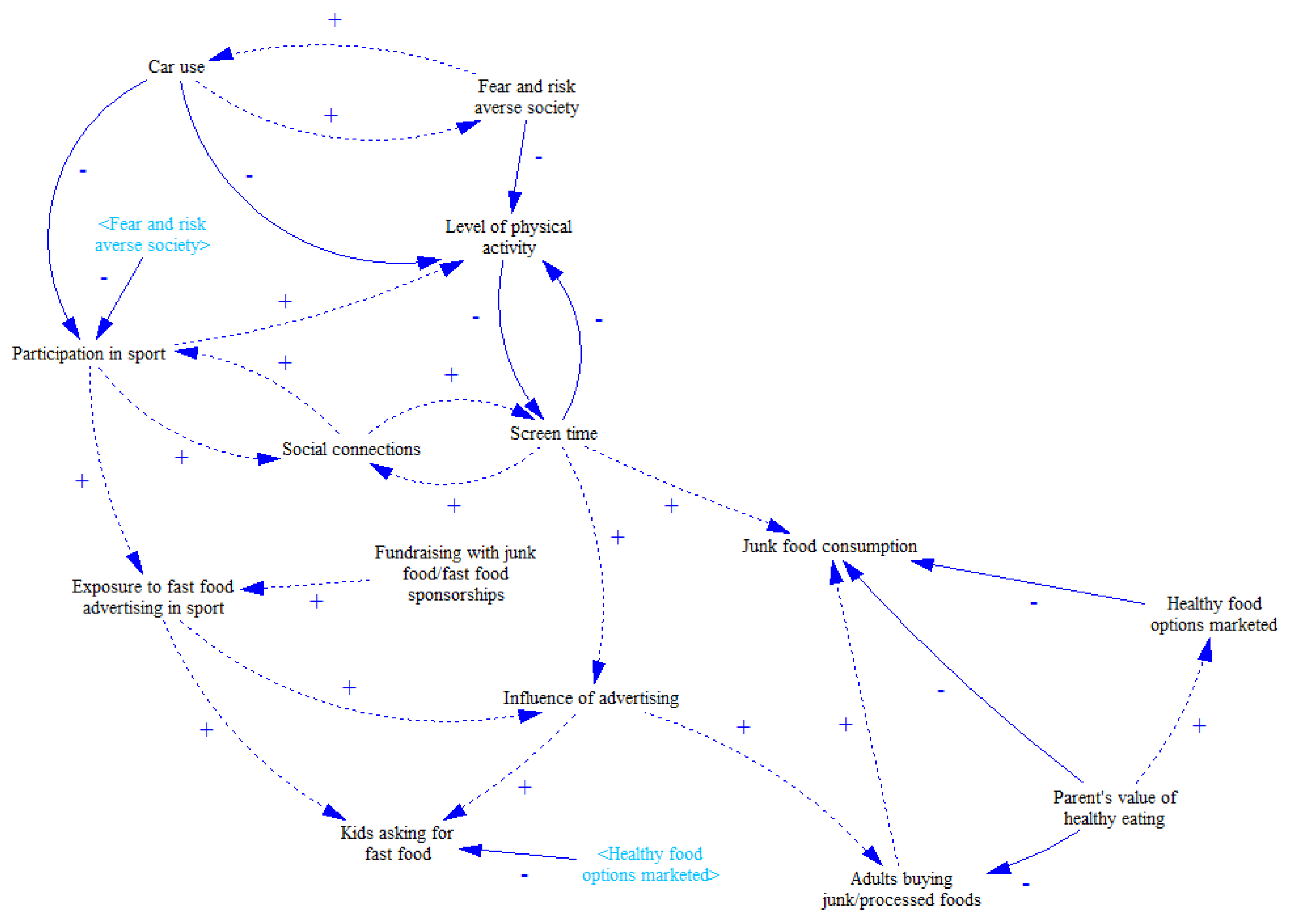
Allender et al. [44] investigated what kind of consensus and insight can a community gain about the problem of childhood obesity using group model building. The final causal loop diagram acquired is presented in Figure 16. Due to the diagram complexity and specific research goals, authors distinguished four main sections of the diagram with colours—these represent social influences, general physical activities, participation in sport, and fast food and junk food. Although this can split the diagram to four mutually interconnected less complex sub-diagrams, this decomposition has its own week points (e.g., quite inappropriate number of blind branches that are difficult to be identified—compare Figure 16 and Figure 17). The colour-based decomposition applied in the original manuscript is not used in reproduction of the diagram as this does not add value to the method application and verification in this study.
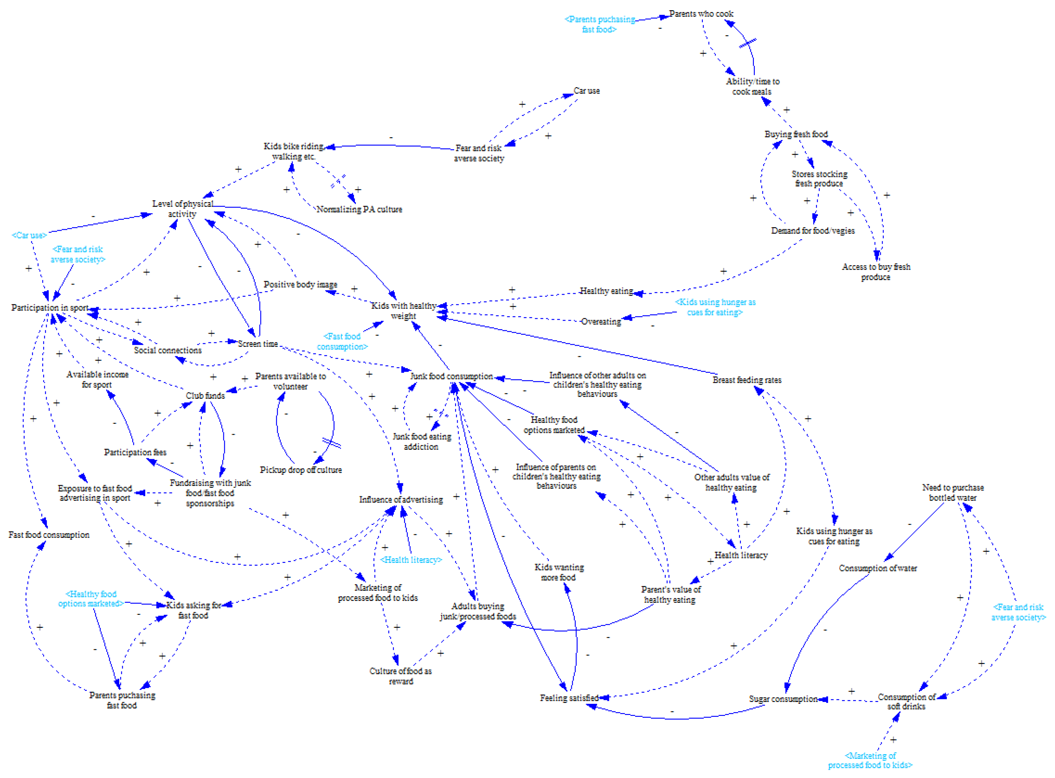
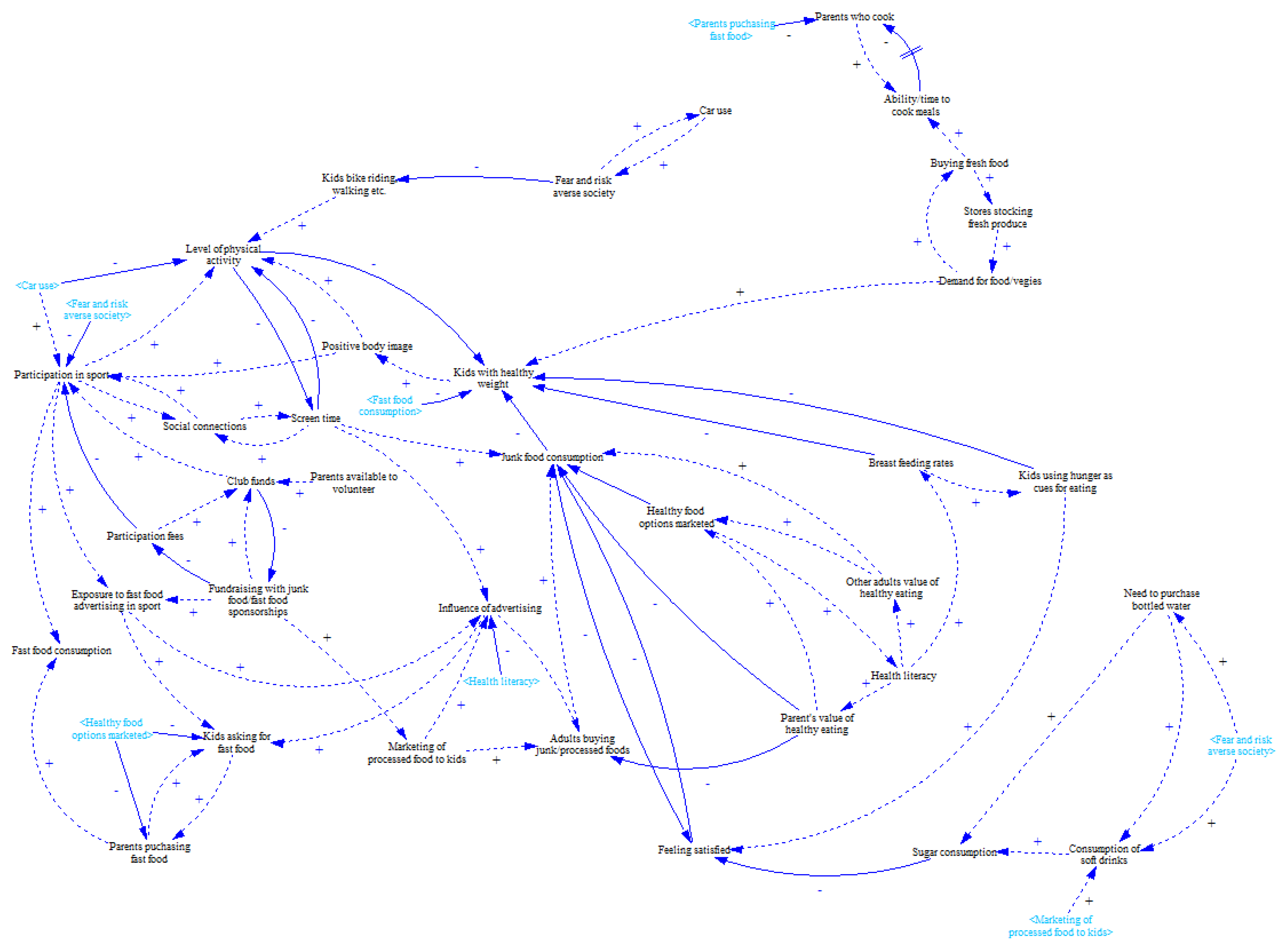
Figure 18, Figure 19 and Figure 20 illustrate the simplification process conducted in the same way as in Case Study 1. Figure 20 represents the final version of the diagram including the most significant MIMO variables as well as inputs and outputs. Local reinforcing feedbacks focused for instance on social life can be identified. Contrary to Case Study 1, the simplification process could have been stopped a little bit earlier here. Although feedbacks are not highlighted there, local feedback loops associated with Participation in sport or Screen time variables are visible. The final version of the causal loop diagram in Figure 20 might be perceived as too simple, which is very likely correct (e.g., causal loop diagram in Figure 19 seems to be more suitable for practical use). Although the simplification process could have been terminated earlier, the intention was to perform exactly the same number of steps in both case studies.
5. Discussion and Limitations
In system dynamics, models that address a large number of “issues of importance in few equations”, or, in other words, models that maximise the number of “insights per equation” are preferred [39]. Although this statement is suitable for quantitative modelling with the help of stock-and-flow diagrams, this idea is applicable to qualitative modelling with causal loop diagrams as well. If the objective of a study is sufficiently clear, a rather powerful small model can be created, and the insights sharply focused [59]. Despite the benefits, small models also have limitations [39]. For instance, customers often demand an exclusive model that considers all possible causal links, either observed or contemplated. In such a situation, trust can be lost if their hypothesized link or variable is not included in the model.
Let us consider small models proven to be valuable. Then, the question about situations in which usability of the presented method can be maximised can arise. In general, qualitative modelling is applied during early stages of the modelling process. It is followed by quantitative modelling, which enables inclusion of mathematical formalism, quantification of parameters and consequent simulation of the model. This sequence is not supported by all system dynamists. For instance, when going back to the pioneering times, Goodman stated that causal loop diagrams should have been used during the stage of conceptualisation [35]. Conceptualisation usually takes place at the beginning of the modelling process. Contrary to this, Morecroft asserted that causal loop diagrams had been argued to be a weak tool of conceptualisation [34]. He claimed that their main strength was in providing an overview of loop structure, which was most useful in behaviour analysis, not conceptualisation. In fact, the role of causal loop diagrams changed over time. Looking back to seminal works published by Jay Forrester, there is no causal loop diagram used in Industrial Dynamics [60]. At the end of the 1960s, it appeared in a form that helped with summarising and explaining the behaviour of fully specified simulation models. Thus, causal loop diagrams were used towards the end of a study to represent and communicate the structure of the dominant loops that had been determined using simulation. However, this approach changed significantly. Diagrams started to be used at the beginning of studies as a conceptualisation tool. The method developed in this manuscript is in concordance with this evolution and considers causal loop diagrams as a tool associated with the conceptualisation stage of the modelling process. Therefore, its application is solely related to qualitative modelling without taking quantitative aspects of a study into consideration. Focus on qualitative aspects is based on Coyle’s conviction that while quantification may indeed offer potential value in many cases, the risks associated with attempting to quantify multiple and poorly understood soft relationships are likely to outweigh whatever potential benefit there might be [61]. Hence, presented simplification method aims at helping with better understanding of a studied system.
In the current form, the method provides outcome that can be used as a valuable mean of introduction and presentation of the modelled system to specific target groups such as modelling workshop newcomers, new team members or decision- or policy-makers that need some kind of initial insight. System modellers can use it in order to simplify the story itself. Moreover, the final version of diagram does not have to represent the only valuable outcome. The whole simplification process can be eventually reversed and applied in the backward direction. This procedure enables to recreated initial complexity, however, in several steps. In this way, continuous growth complexity is presented to the same target group, which enables to tame complexity as well. Hence, the more appropriate and precise system comprehension can be anticipated.
In comparison to already existing simplification methods outlined at the beginning of this manuscript, the new presented method possesses various advantages or similarities. For instance, the main limitation of the method developed by Franek et al. [43] is its exclusive association with diagrams created digitally. The method is not able to help with diagrams produced with the help of pen and paper, which represents common practice during modelling workshops [43]. However, both methods are based on preference of significant system elements as centrality and MIMOs have very close meaning. Saysel and Barlas present their approach to simplification which is however associated with quantitative modelling as the main criterion of simplification is based on comparison whether an elimination of a model structure results in a loss of any of the reference behaviours, validation or policy/scenario runs [37]. Although their method can be considered as a valuable contribution, the verification technique disqualifies it from application in qualitative modelling. Moreover, authors do not explicitly state the main value on which the method is built. Nevertheless, its iterative feature grounded in repetition of selected steps unless the model does not meet the selected criterion is shared by both methods. Moreover, its first and second steps are based on similar principles as endogenisation and encapsulation procedures. Finally, it is quite complicated to compare the new method with approach introduced by Eberlein as it is focused on stock and flow diagrams, its application is restricted to linearized models, and grounded in mathematical formalism and reasoning without available case study [42].
There are various limitations associated with the method application. First, successfulness of the simplification process was verified by ten individuals attending Case Study 1 only. Rigorous experimental evaluation of suitability based on a larger sample of users’ needs to be conducted. The experiment should follow the traditional pre- and post-application assessment of coherence and conformity with users’ perspectives.
Second, although the complexity of diagrams used in case studies is relatively high, further verification of different complexity scales of a diagram should be performed.
Third, it is demonstrated in this study that the simplification method is appropriate for group diagrams. The appropriateness is grounded in multiple perspectives of all modellers who are aware of necessity to reach consensus [62]. Even if greater accuracy or an expanded boundary is ultimately necessary, the success of such efforts will often depend on the consensus that is first built through a smaller model [39]. In the case of complex individual diagrams, this procedure will not be very likely accepted, as any modeller can simplify his/her own diagram just by removal of variables that have the least importance from his/her point of view. There is no need to achieve the consensus. Last, although causal loop diagrams are mostly used for modelling of soft systems, its limited possibility for implementation in the hard system domain should be mentioned. In the case of hard systems (e.g., technical devices), all variables and links are quite strictly and rigorously defined. Any simplification can lead to a vague description that can be helpful only in limited number of occasions (e.g., explanation of the system behaviour to a user beginner). In this realm, e.g., in systems engineering, the simplification of diagrams is a subject of critique by practitioners [63]. Nevertheless, as already stated, the application of causal loop diagrams in the realm of hard disciplines is rare. The diagrams are mostly used for modelling of complex soft systems in which simplifications are acceptable due to less rigorous definition and determination of variables and their links.
6. Further Research Directions
Coping with aforementioned limitations opens new research pathways. Once the usability is rigorously verified, it should be reasonable to automate the process and apply it in practice with the help of a proprietary software application. This would enable the further development of the method itself. For instance, a software application can be capable of monitoring feedback loops and giving them a preference during the method execution. Moreover, required complexity could be determined by number of feedbacks, not only by number of variables and links. This indicator can be considered as more appropriated for system dynamics models. It is practically impossible to achieve this manually due to the overwhelming complexity that the method has an ambition to deal with. Because causal loop diagrams are created with help of many tools (white board, pen and paper, graphical software packages, etc.) which are only graphical in their nature, the biggest challenge here would be both transformation of the diagram structure in the more formal representation, e.g., incidence matrix, and bridging SISO variables. Furthermore, the method can be extended by more sophisticated techniques such as dominant assessment of feedback loops [64] which is focused on dominant loop analysis. Identification of the most dominant feedbacks that contribute most to a particular behaviour or behaviour change would enable removal of feedbacks that are less important.
7. Conclusions
Complexity represents an issue in many research disciplines. System dynamics is not an exception. It does not deal only with the complex phenomena, but it also incorporates dynamics, which brings more difficulty into our ability to understand the modelled systems. Two types of diagrams prevail in system dynamics, where causal loop diagrams represent the main research construct of this study. Increasingly complex causal diagrams are being to include all relevant variables. Although the complexity can be described by several indicators, the number of variables and links included in the diagram are used as the main complexity measure in this study. Making diagram more complex has negative consequences ranging from time demands during the development process to reduced comprehensibility during diagram interpretation and analysis. Forrester argues that small models are powerful [59]. Heeding Forrester’s argument, this manuscript introduces the original systematic method of the simplification that can be successfully applied in practice. It is iterative in its nature and is grounded in three specific activities: endogenisation, encapsulation, and order-oriented reduction. All three activities focus on preference of multi-input and multi-output variables. List of initial inputs and outputs and the simplified version of causal loop diagrams represent two main method outcomes. Two presented case studies verify method’s usability and applicability. This opens new research directions that can be realised in the future. Although there are some limitations associated with the method, they can be successfully resolved in the near future. In this way, a valuable tool for those who cope with complexity of causal loop diagrams in practice is offered.
Acknowledgments
The financial support of the Specific Research Project “Autonomous Socio-Economic Systems” of FIM UHK is gratefully acknowledged. The author would like to thank Tomáš Nacházel for his responsiveness and help.
Conflicts of Interest
The author declares no conflict of interest. The founding sponsors had no role in the design of the study; in the collection, analyses, or interpretation of data; in the writing of the manuscript, and in the decision to publish the results.
References
- Miller, G.A. The magical number seven, plus or minus two: Some limits on our capacity for processing information. Psychol. Rev. 1956, 63, 81–97. [Google Scholar] [CrossRef] [PubMed]
- Corbett, E.A.; Smith, P.L. The Magical Number One-on-Square-Root-Two: The Double-Target Detection Deficit in Brief Visual Displays. J. Exp. Psychol. Hum. Percept. Perform. 2017, 47, 1376–1396. [Google Scholar] [CrossRef] [PubMed]
- Konstantinou, N.; Constantinidou, F.; Kanai, R. Discrete capacity limits and neuroanatomical correlates of visual short-term memory for objects and spatial locations. Hum. Brain Mapp. 2017, 38, 767–778. [Google Scholar] [CrossRef] [PubMed]
- Cowan, N. The magical number 4 in short-term memory: A reconsideration of mental storage capacity. Behav. Brain Sci. 2001, 24, 87–185. [Google Scholar] [CrossRef] [PubMed]
- Keogh, R.; Pearson, J. The perceptual and phenomenal capacity of mental imagery. Cognition 2017, 162, 124–132. [Google Scholar] [CrossRef] [PubMed]
- Saaty, T.L. Why the magic number seven plus or minus two. Math. Comput. Model. 2003, 38, 233–244. [Google Scholar] [CrossRef]
- Gell-Mann, M. What Is Complexity? In Complexity and Industrial Clusters: Dynamics and Models in Theory and Practice; Curzio, A.Q., Fortis, M., Eds.; Physica-Verlag: Heidelberg, Germany, 2002; pp. 13–24. ISBN 978-3-7908-1471-2. [Google Scholar]
- Viana, A. Vico, Peirce, and the issue of complexity in human sciences. Cogn. Semiot. 2017, 10, 1–18. [Google Scholar] [CrossRef]
- Adami, C. What is complexity? BioEssays 2002, 24, 1085–1094. [Google Scholar] [CrossRef] [PubMed]
- Łapa, K.; Zalasiński, M.; Cpałka, K. A new method for designing and complexity reduction of neuro-fuzzy systems for nonlinear modelling International. In Lecture Notes in Artificial Intelligence; Rutkowski, L., Korytkowski, M., Scherer, R., Tadeusiewicz, R., Zadeh, L.A., Zurada, J.M., Eds.; Springer: Heidelber, Germany, 2013; pp. 329–344. ISBN 978-3-642-38657-2. [Google Scholar]
- Diodato, N.; Brocca, L.; Bellocchi, G.; Fiorillo, F.; Guadagno, F.M. Complexity-reduction modelling for assessing the macro-scale patterns of historical soil moisture in the Euro-Mediterranean region. Hydrol. Process. 2014, 28, 3752–3760. [Google Scholar] [CrossRef]
- Mesmin, C.; van Oostrum, J.; Domon, B. Complexity reduction of clinical samples for routine mass spectrometric analysis. Proteom. Clin. Appl. 2016, 10, 315–322. [Google Scholar] [CrossRef] [PubMed]
- Patton, M.Q. Developmental Evaluation: Applying Complexity Concepts to Enhance Innovation and Use; Guilford Press: New York, NY, USA, 2011; ISBN 978-1-606-23872-1. [Google Scholar]
- Hassmiller Lich, K.; Ginexi, E.M.; Osgood, N.D.; Mabry, P.L. A call to address complexity in prevention science research. Prev. Sci. 2013, 14, 279–289. [Google Scholar] [CrossRef] [PubMed]
- Luke, D.A.; Stamatakis, K.A. Systems science methods in public health: Dynamics, networks, and agents. Annu. Rev. Public Health 2012, 33, 357–376. [Google Scholar] [CrossRef] [PubMed]
- Tozan, Y.; Ompad, D.C. Complexity and dynamism from an urban health perspective: A rationale for a system dynamics approach. J. Urban Health 2015, 92, 490–501. [Google Scholar] [CrossRef] [PubMed]
- Senge, P.M. The Fifth Discipline: The Art and Practice of the Learning Organization; Doubleday/Currency: New York, NY, USA, 2006; ISBN 0-385-51725-4. [Google Scholar]
- Richmond, B.; Peterson, S. An Introduction to Systems Thinking; High Performance Systems, Inc.: Lebanon, NH, USA, 2001; ISBN 0-9704921-1-1. [Google Scholar]
- Sterman, J.D. Learning from evidence in a complex world. Am. J. Public Health 2006, 96, 505–514. [Google Scholar] [CrossRef] [PubMed]
- Lakeh, A.B.; Ghaffarzadegan, N. Does analytical thinking improve understanding of accumulation? Syst. Dyn. Rev. 2015, 31, 46–65. [Google Scholar] [CrossRef]
- McGlashan, J.; Johnstone, M.; Creighton, D.; de la Haye, K.; Allender, S. Quantifying a Systems Map: Network Analysis of a Childhood Obesity Causal Loop Diagram. PLoS ONE 2016, 11, e0165459. [Google Scholar] [CrossRef] [PubMed]
- Ison, R. Systems Practice: How to Act in a Climate-Change World; Springer: London, UK, 2010; ISBN 978-1-84996-124-0. [Google Scholar]
- Mabry, P.L.; Kaplan, R.M. Systems Science: A Good Investment for the Public’s Health. Health Educ. Behav. 2013, 40, 9S–12S. [Google Scholar] [CrossRef] [PubMed]
- Vugteveen, P.; Rouwette, E.; Stouten, H.; van Katwijk, M.M.; Hanssen, L. Developing social-ecological system indicators using group model building. Ocean Coast. Manag. 2015, 109, 29–39. [Google Scholar] [CrossRef]
- Jun, H.-B.; Kim, D. A Bayesian network-based approach for fault analysis. Expert Syst. Appl. 2017, 81, 332–348. [Google Scholar] [CrossRef]
- Bureš, V.; Tučník, P. Complex Agent-Based Models: Application of a Constructivism in the Economic Research. E+M Ekon. Manag. 2014, 17, 152–168. [Google Scholar] [CrossRef]
- Hassmiller Lich, K.; Urban, J.B.; Frerichs, L.; Dave, G. Extending systems thinking in planning and evaluation using group concept mapping and system dynamics to tackle complex problems. Evaluation Program Plan. 2017, 60, 254–264. [Google Scholar] [CrossRef] [PubMed]
- Hajek, P.; Michalak, K. Feature selection in corporate credit rating prediction. Knowl. Based Syst. 2013, 51, 72–84. [Google Scholar] [CrossRef]
- Kelly, R.A.; Jakeman, A.J.; Barreteau, O.; Borsuk, M.E.; ElSawah, S.; Hamilton, S.H.; Henriksen, H.J.; Kuikka, S.; Maier, H.R.; Rizzoli, A.E.; et al. Selecting among five common modelling approaches for integrated environmental assessment and management. Environ. Model. Softw. 2013, 47, 159–181. [Google Scholar] [CrossRef]
- Loyo, H.K.; Batcher, C.; Wile, K.; Huang, P.; Orenstein, D.; Milstein, B. From model to action: Using a system dynamics model of chronic disease risks to align community action. Health Promot. Pract. 2013, 14, 53–61. [Google Scholar] [CrossRef] [PubMed]
- Mavrommati, G.; Bithas, K.; Panayiotidis, P. Operationalizing sustainability in urban coastal systems: A system dynamics analysis. Water Res. 2013, 47, 7235–7250. [Google Scholar] [CrossRef] [PubMed]
- Groesser, S.N.; Schaffernicht, M. Mental models of dynamic systems: Taking stock and looking ahead. Syst. Dyn. Rev. 2012, 28, 46–68. [Google Scholar] [CrossRef]
- Hovmand, P. Community Based System Dynamics; Springer: New York, NY, USA, 2013; ISBN 978-1-4939-4386-9. [Google Scholar]
- Morecroft, J.D.W. A critical review of diagraming tools for conceptualizing feedback system model. Dynamica 1982, 8, 20–29. [Google Scholar]
- Goodman, M.R. Study Notes in System Dynamics; MIT Press: Cambridge, MA, USA, 1974; ISBN 0-914700-00-6. [Google Scholar]
- Richardson, G.P. Problems with causal-loop diagrams. Syst. Dyn. Rev. 1986, 2, 158–170. [Google Scholar] [CrossRef]
- Saysel, A.K.; Barlas, Y. Model simplification and validation with indirect structure validity tests. Syst. Dyn. Rev. 2006, 22, 241–262. [Google Scholar] [CrossRef]
- Sterman, J.D. Business Dynamics: Systems Thinking and Modeling for a Complex World; Irwin/McGraw-Hill: Boston, MA, USA, 2000. [Google Scholar]
- Ghaffarzadegan, N.; Lyneis, J.; Richardson, G.P. How small system dynamics models can help the public policy process. Syst. Dyn. Rev. 2011, 27, 22–44. [Google Scholar] [CrossRef]
- Yao, Z.; Wu, L.; Song, H. Problems of network simplification by edge bundling. J. Beijing Univ. Aeronaut. Astronaut. 2015, 41, 871–878. [Google Scholar]
- Du, F.; Xuan, Q.; Wu, T.J. Simplification of complex networks by folding. In Proceedings of the 29th Chinese Control Conference, Beijing, China, 29–31 July 2010; pp. 4667–4670. [Google Scholar]
- Eberlein, R.L. Simplification and understanding of models. Syst. Dyn. Rev. 1989, 5, 51–68. [Google Scholar] [CrossRef]
- Frannek, L.; Nagaoka, H.; Nakagawa, T. Network simplification and visualization through System Dynamics-based network centrality. In Proceedings of the 34th International Conference of the System Dynamics Society, Delft, The Netherlands, 17–21 July 2016; pp. 1–19. [Google Scholar]
- Allender, S.; Owen, B.; Kuhlberg, J.; Lowe, J.; Nagorcka-Smith, P.; Whelan, J.; Bell, C. A Community Based Systems Diagram of Obesity Causes. PLoS ONE 2015, 10, e0129683. [Google Scholar] [CrossRef] [PubMed]
- Inam, A.; Adamowski, J.; Halbe, J.; Prasher, S. Using causal loop diagrams for the initialization of stakeholder engagement in soil salinity management in agricultural watersheds in developing countries: A case study in the Rechna Doab watershed, Pakistan. J. Environ. Manag. 2015, 152, 251–267. [Google Scholar] [CrossRef] [PubMed]
- Conroy, S.A.; Gupta, N. Team Pay-For-Performance: The Devil is in the Details. Group Organ. Manag. 2016, 41, 32–65. [Google Scholar] [CrossRef]
- Roubos, H.; Setnes, M. Compact and transparent fuzzy models and classifiers through iterative complexity reduction. IEEE Trans. Fuzzy Syst. 2001, 9, 516–524. [Google Scholar] [CrossRef]
- Scott, R.J.; Cavana, R.Y.; Cameron, D. Recent evidence on the effectiveness of group model building. Eur. J. Oper. Res. 2016, 249, 908–918. [Google Scholar] [CrossRef]
- Vennix, J.A.M. Group Model Building: Facilitating Team Learning Using System Dynamics; Wiley: Chichester, UK, 1996; ISBN 978-0-471-95355-5. [Google Scholar]
- Andersen, D.; Richardson, G. Scripts for group model building. Syst. Dyn. Rev. 1997, 13, 107–129. [Google Scholar] [CrossRef]
- Bureš, V.; Racz, F. Application of system archetypes in practice: An underutilised pathway to better managerial performance. J. Bus. Econ. Manag. 2016, 17, 1081–1096. [Google Scholar] [CrossRef]
- Morton, A.; Ackermann, F.; Belton, V. Technology-driven and model-driven approaches to group decision support: Focus, research philosophy and key concepts. Eur. J. Inf. Syst. 2003, 12, 110–126. [Google Scholar] [CrossRef]
- Andersen, D.F.; Vennix, J.A.M.; Richardson, G.P.; Rouwette, E.A.J.A. Group model building: Problem structuring, policy simulation and decision support. J. Oper. Res. Soc. 2007, 58, 691–694. [Google Scholar] [CrossRef]
- Richardson, G.P. Concept models in group model building. Syst. Dyn. Rev. 2013, 29, 42–55. [Google Scholar] [CrossRef]
- Rouwette, E.A.J.A.; Bastings, I.; Blokker, H. A comparison of group model building and strategic options development and analysis. Group Decis. Negot. 2011, 20, 781–803. [Google Scholar] [CrossRef]
- Nguyen, T.; Cook, S.; Ireland, V. Application of System Dynamics to Evaluate the Social and Economic Benefits of Infrastructure Projects. Systems 2017, 5, 29. [Google Scholar] [CrossRef]
- Chen, H.; Chang, Y.C.; Chen, K.C. Integrated wetland management: An analysis with group model building based on system dynamics model. J. Environ. Manag. 2014, 146, 309–319. [Google Scholar] [CrossRef] [PubMed]
- Narayanan, V.K.; Armstrong, D.J. Causal Mapping for Research in Information Technology; Idea Publishing Group: Hershey, PA, USA, 2005; ISBN 978-1-591-40396-8. [Google Scholar]
- Forrester, J.W. System dynamics: The next fifty years. Syst. Dyn. Rev. 2007, 23, 359–370. [Google Scholar] [CrossRef]
- Lane, D.C. Diagramming conventions in System Dynamics. J. Oper. Res. Soc. 2000, 51, 241–246. [Google Scholar] [CrossRef]
- Coyle, G. Rejoinder to Homer and Oliva. Syst. Dyn. Rev. 2001, 17, 357–363. [Google Scholar] [CrossRef]
- Franco, L.A.; Rouwette, E.A.J.A.; Korzilius, H. Different paths to consensus? The impact of need for closure on model-supported group conflict management. J. Oper. Res. 2014, 249, 878–889. [Google Scholar] [CrossRef]
- Douglass, B.P. Agile Systems Engineering; Morgan Kaufman: Waltham, MA, USA, 2016; ISBN 978-0-12-802120-0. [Google Scholar]
- Oliva, R.; Mojtahedzadeh, M.T. Keep it simple: A dominance assessment of feedback loops. In Proceedings of the 22nd International Conference of the System Dynamics Society, Oxford, UK, 25–29 July 2004; p. 148. [Google Scholar]
Figure 1.
Individual causal loop diagrams (1).
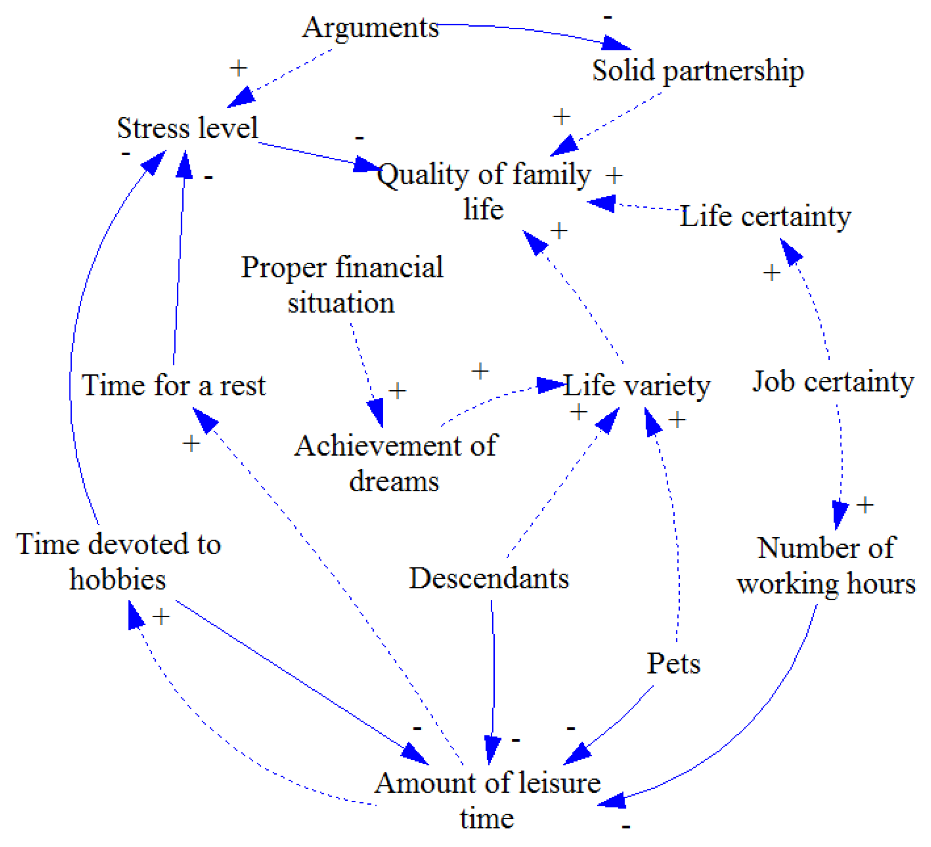
Figure 2.
Individual causal loop diagrams (2).

Figure 3.
Individual causal loop diagrams (3).
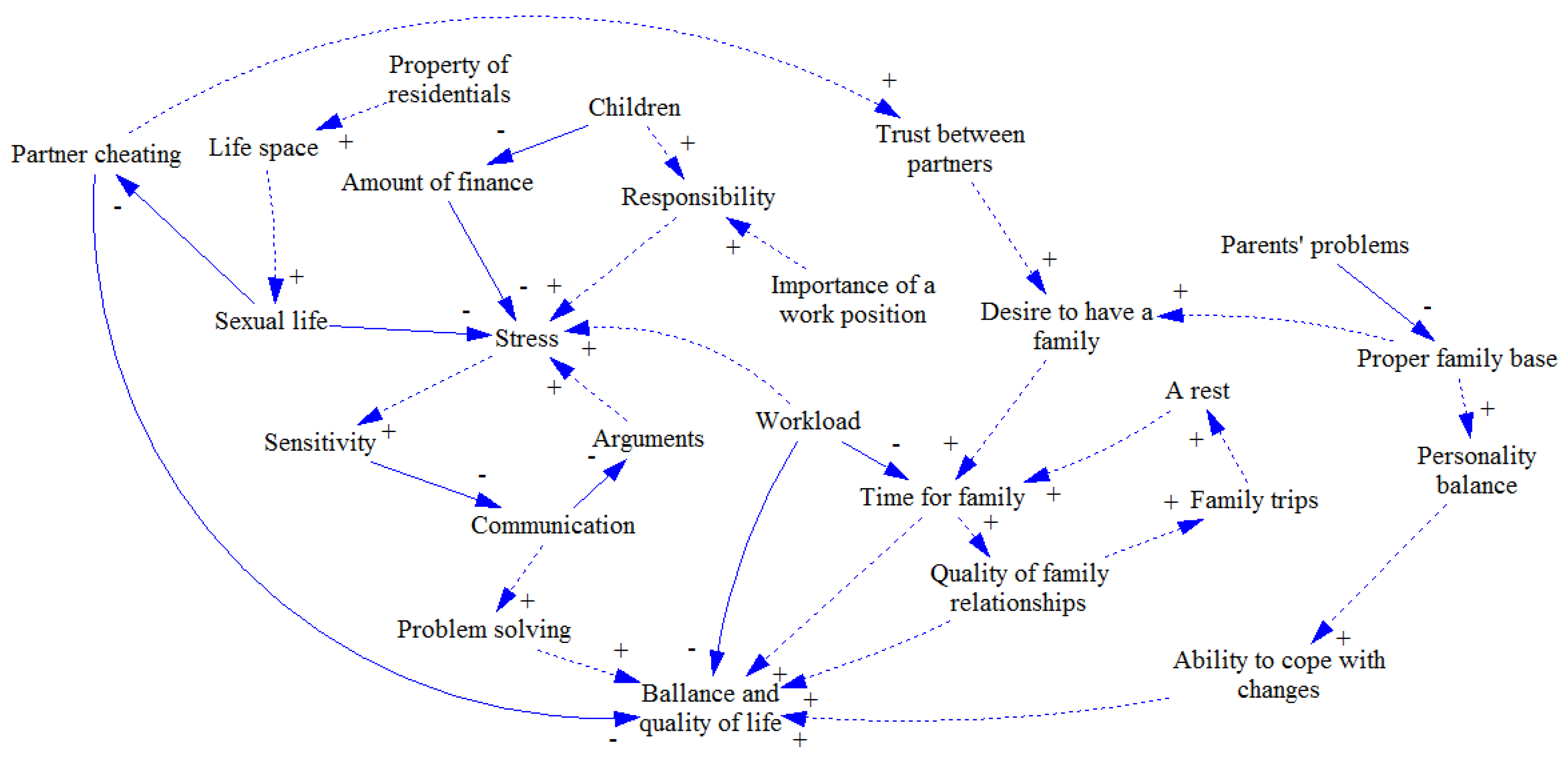
Figure 4.
Individual causal loop diagrams (4).

Figure 5.
Individual causal loop diagrams (5).
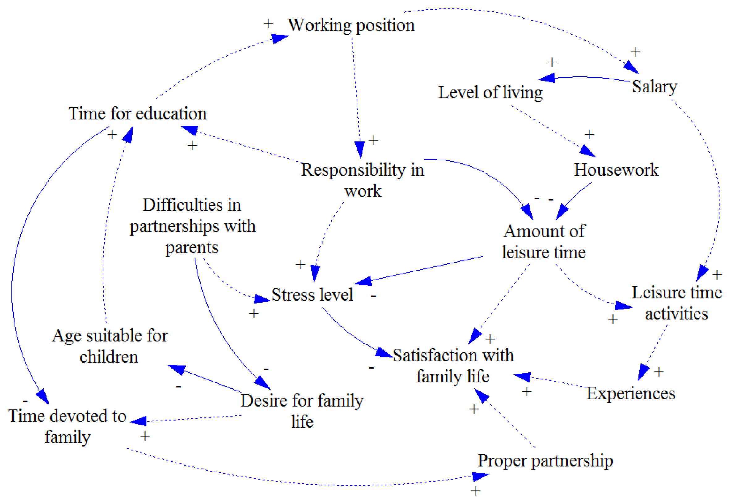
Figure 6.
Individual causal loop diagrams (6).

Figure 7.
Individual causal loop diagrams (7).

Figure 8.
Individual causal loop diagrams (8).

Figure 9.
Individual causal loop diagrams (9).

Figure 10.
Individual causal loop diagrams (10).

Figure 11.
Group causal loop diagram.
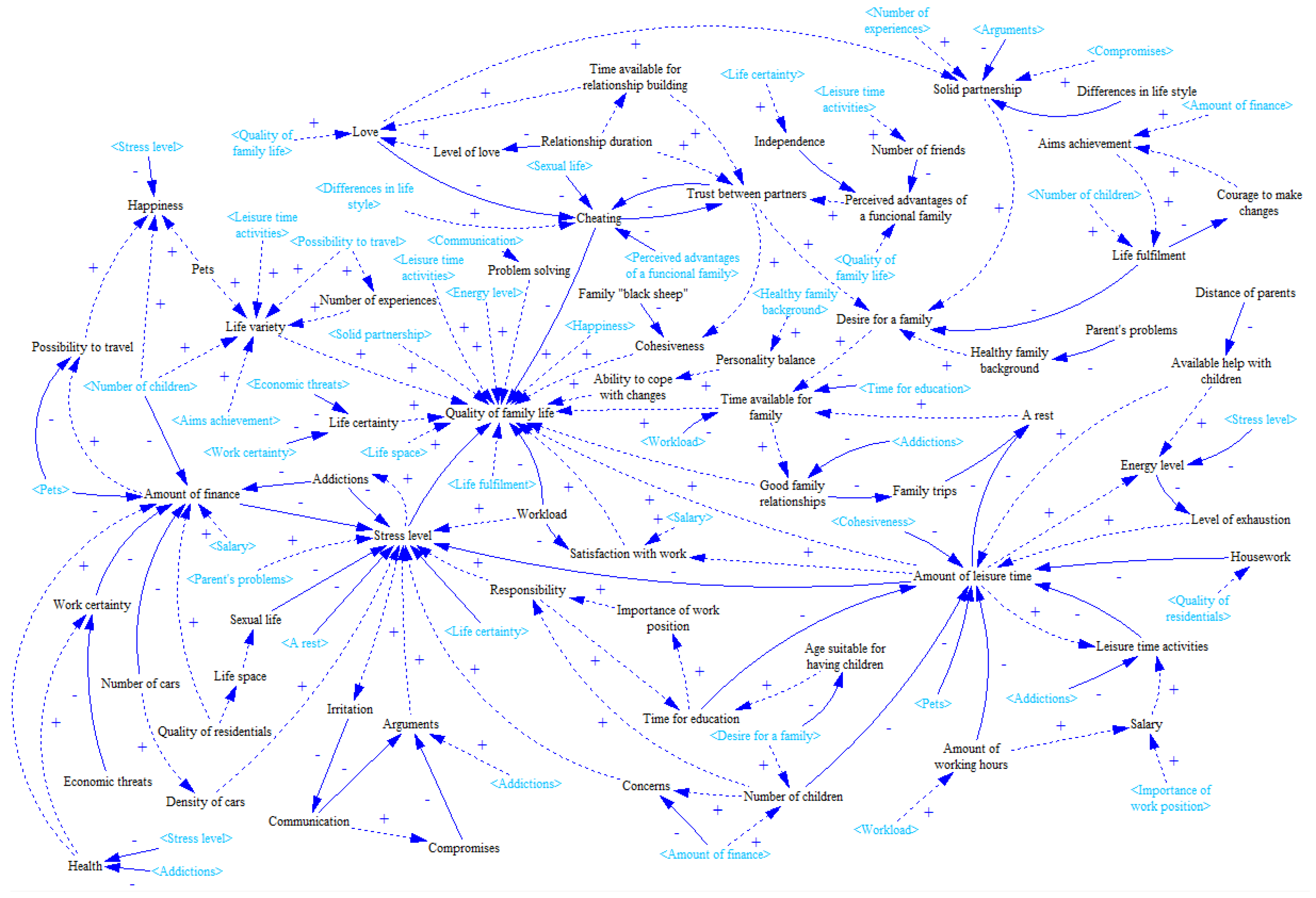
Figure 12.
Result of Step 5.

Figure 13.
Result of Step 7.

Figure 14.
Result of Step 12.
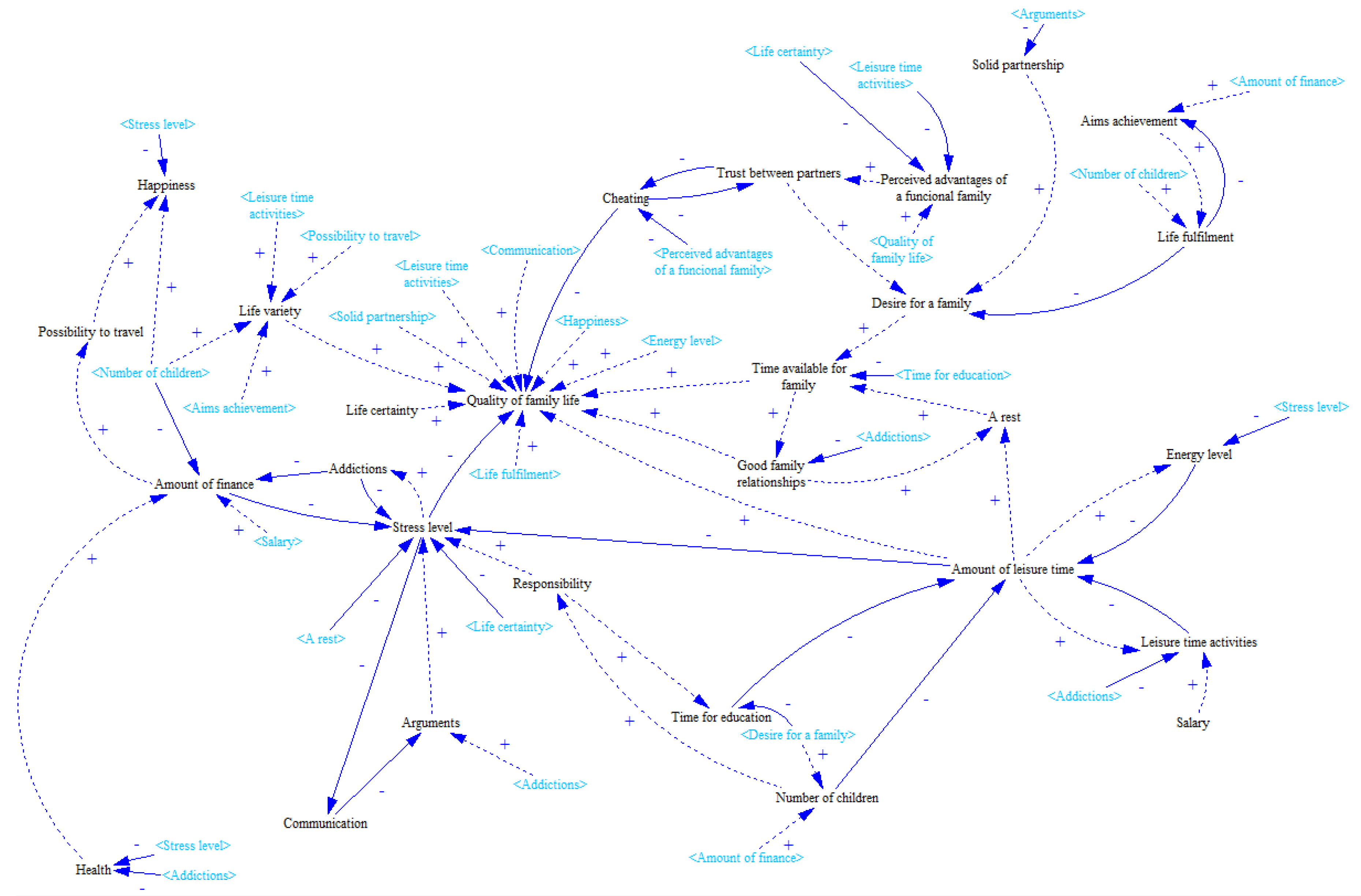
Figure 15.
Final version of the causal loop diagram.

Figure 16.
Full version the causal loop diagram (redrawn based on the diagram presented in [44]).
Figure 16.
Full version the causal loop diagram (redrawn based on the diagram presented in [44]).

Figure 17.
Result of Step 5.

Figure 18.
Result of Step 7.

Figure 19.
Result of Step 12.

Figure 20.
Final version of the causal loop diagram.
© 2017 by the author. Licensee MDPI, Basel, Switzerland. This article is an open access article distributed under the terms and conditions of the Creative Commons Attribution (CC BY) license (http://creativecommons.org/licenses/by/4.0/).
Share and Cite
MDPI and ACS Style
Bureš, V. A Method for Simplification of Complex Group Causal Loop Diagrams Based on Endogenisation, Encapsulation and Order-Oriented Reduction. Systems 2017, 5, 46. https://doi.org/10.3390/systems5030046
AMA Style
Bureš V. A Method for Simplification of Complex Group Causal Loop Diagrams Based on Endogenisation, Encapsulation and Order-Oriented Reduction. Systems. 2017; 5(3):46. https://doi.org/10.3390/systems5030046
Chicago/Turabian StyleBureš, Vladimír. 2017. "A Method for Simplification of Complex Group Causal Loop Diagrams Based on Endogenisation, Encapsulation and Order-Oriented Reduction" Systems 5, no. 3: 46. https://doi.org/10.3390/systems5030046
Note that from the first issue of 2016, this journal uses article numbers instead of page numbers. See further details here.