THz/Infrared Double Resonance Two-Photon Spectroscopy of HD+ for Determination of Fundamental Constants

Laboratoire PhLAM, CNRS UMR 8523, 59655 Villeneuve d’Ascq, France
Atoms 2017, 5(4), 38; https://doi.org/10.3390/atoms5040038
Submission received: 1 September 2017
/
Revised: 1 October 2017
/
Accepted: 6 October 2017
/
Published: 12 October 2017
(This article belongs to the Special Issue High Precision Measurements of Fundamental Constants)
Abstract
:A double resonance two-photon spectroscopy scheme is discussed to probe jointly rotational and rovibrational transitions of ensembles of trapped HD+ ions. The two-photon transition rates and lightshifts are calculated with the two-photon tensor operator formalism. The rotational lines may be observed with sub-Doppler linewidth at the hertz level and good signal-to-noise ratio, improving the resolution in HD+ spectroscopy beyond the 10−12 level. The experimental accuracy, estimated at the 10−12 level, is comparable with the accuracy of theoretical calculations of HD+ energy levels. An adjustment of selected rotational and rovibrational HD+ lines may add clues to the proton radius puzzle, may provide an independent determination of the Rydberg constant, and may improve the values of proton-to-electron and deuteron-to-proton mass ratios beyond the 10−11 level.
1. Introduction
Precision measurements with atoms and molecules improved our understanding of the structure of matter and of its interaction with light. Predictions of the quantum electrodynamics (QED) were compared with accurate experimental data to test the validity of the theory and to extract the values of fundamental constants [1]. Precision spectroscopy of atomic hydrogen and deuterium is used to extract the Rydberg constant, the proton radius, and the deuteron radius. Significant discrepancies were noticed between the proton radius and the deuteron radius determined from regular (electronic) hydrogen and deuterium and from exotic (muonic) hydrogen and deuterium, respectively [2]. This problem, called “the proton radius puzzle”, motivated several works [3]. The agreement between independent determinations of physical constants may check the validity of theoretical and experimental results. Moreover, space-time variations of fundamental constants are allowed in theories beyond the Standard Model (see [4] for a review). Constraints on possible variation of the proton-to-electron mass ratio were derived from astrophysical spectra or laboratory studies (see for example [5]).
The hydrogen molecular ions are the simplest molecules. They have an important role in molecular quantum mechanics [6]. High-resolution infrared spectroscopy associated with accurate ab-initio calculations open the way to applications for the determination of fundamental constants and for testing QED [7]. QED calculations of the energy levels of the hydrogen molecular ions were performed including corrections up to the mα8 order [8,9,10,11] and reduced the relative uncertainty for fundamental vibrational transitions to 7.6 × 10⁻¹². Accurate experimental results were obtained using hydrogen molecular ions stored in radiofrequency (r.f.) traps and sympathetically cooled by laser-cooled Be+ ions. In addition, it is possible to efficiently prepare HD+ ions in the fundamental rotational level [12,13]. Weak rovibrational overtone transitions are allowed by electrical-quadrupole coupling for H2+ ions and by electrical-dipole coupling for HD+ ions. The natural linewidths of the rovibrational transitions are at the 10 Hz level for HD+ and the 10−7 Hz level for H2+ [14]. The systematic frequency shifts were accurately calculated for hydrogen molecular ions [15,16]. The experimental accuracy with a dipole-allowed rovibrational overtone transition of HD+ was 1.1 × 10⁻⁹ [17]. The agreement with theoretical results at 1.1 × 10⁻⁹ allowed a test of QED, provided a determination of the proton-to-electron mass ratio, as suggested by [18], and constrained the effect of “fifth forces” [19]. The experimental uncertainty of HD+ ion lines was limited by Doppler broadening. Doppler-free two-photon spectroscopy of a rovibrational overtone transition of HD+ was proposed to improve the uncertainty beyond the 1 × 10⁻¹² level [20]. In this approach, efficient two-photon excitation in HD+ is provided by driving a pair of dipole-allowed E1-E1 rovibrational transitions with lasers tuned close to resonance with an intermediate energy level. The trapped HD+ ions are in the Lamb-Dicke regime, as their oscillatory motion in the trap is confined over a distance smaller than the effective laser wavelength, that allows to probe the two-photon transition virtually without Doppler and recoil effects. The advantage of the two-photon spectroscopy approach is to suppress the first-order Doppler effect even without strong spatial confinement. The observation of an electric-quadrupole allowed E2 transition for homonuclear diatomic ions, demonstrated with N2+ [21], may be an alternative to increase the accuracy with Doppler-free spectroscopy in the Lamb-Dicke regime.
This contribution proposes to determine the Rydberg constant, the nuclear-to-electron mass ratios, and the nuclear radii using Doppler-free spectroscopy of hydrogen molecular ions. A THz/infrared double resonance two-photon spectroscopy study on trapped HD+ ions may allow joint measurements of E1-E1 rotational transitions in the vibrational ground state and of E1-E1 rovibrational transitions with different sensitivities on fundamental constants. The rotational levels in the vibrational ground state have long (1 s level) radiative lifetimes, compared to 10 ms level lifetimes of excited rovibrational levels, that may lead to an improvement of the resolution beyond the 10−12 level. Efficient detection of molecular transitions may be provided by state-selective resonance-enhanced multiphoton dissociation (REMPD) [20]. The double resonance spectroscopy scheme, proposed here, based on (v,L) = (0,1)→(0,3) and (v,L) = (0,3)→(9,3) two-photon transitions, may provide complementary experimental data to previous microwave/infrared double resonance studies on HD+ ion beams [6]. This article addresses the hyperfine structure of the rovibrational energy levels to calculate two-photon transition rates and lightshifts with the two-photon tensor operator formalism [22]. The lineshapes obtained in the double resonance two-photon spectroscopy scheme are determined using a rate equation model that describes the interaction with the blackbody radiation (BBR). The frequency stability, the Zeeman shift, and the lightshift are evaluated for a molecular clock based on HD+ two-photon rotational lines. Finally, the determination of fundamental constants is discussed.
2. Two-Photon Tensor Formalism Calculations
2.1. Hyperfine Structure of Rovibrational Energy Levels of HD+
The HD+ ion is formed with particles that have non-zero spins. The rovibrational energy levels, calculated in the nonrelativistic approximation [23], have a hyperfine structure due to various spin-spin and spin-orbit interactions. The spin coupling scheme is that used in [24]:
where the electron, proton, and deuteron spin operators are, respectively, , , and , is the rotational angular momentum operator, and is the total angular momentum operator.
The basis vectors |vLFSJ> are expressed in terms of the vibrational quantum number v and the eigenvalues of , , , and . In this pure basis, J is the only good quantum number, but L is also used for labelling the levels as the hyperfine spacing is smaller than the rotational structure. An effective spin Hamiltonian is taken for the hyperfine structure of each rotational level. The spin Hamiltonian is expressed in a simplified form [6]:
accounting for the Fermi contact and magnetic dipolar hyperfine interactions for the proton and the deuteron and for the spin-rotation interaction. The values for the parameters bH, cH, and γ have been calculated in [24]. The other parameters are estimated as bD = (gd/gp)bH and cD = (gd/gp)cH with the gyromagnetic factors of the proton and of the deuteron from CODATA 2014 recommended values of the fundamental physical constants [1].
The eigenvectors |vLn> of the mixed basis are labelled with an integer n and expressed as a linear combination of the pure basis eigenvectors:
The diagonalisation of the effective spin Hamiltonian yields a set of coefficients and eigenvalues ΔEv,L,n relative to the hyperfine-free rotational level energy.
The L = 0,L = 1, and L ≥ 2 rotational levels have, respectively, 4, 10, and 12 hyperfine structure levels with splittings < 1 GHz. The most important splitting, between (F,S) = (1,0) and (F,S) = (0,1) levels, is determined by the proton-electron spin-spin interaction. The calculations with this simplified Hamiltonian lead to hyperfine energy levels frequency shifted by ≤ 33 kHz to the hyperfine levels calculated in [24]. The frequency shifts of the hyperfine-free rotational frequencies are expected to be orders of magnitude smaller because of the differential effects of the hyperfine couplings.
In presence of a magnetic field, the hyperfine levels are split into sublevels |vLnJz> labelled by the quantum number Jz of the projection of on the field axis. The Zeeman Hamiltonian can be expressed with terms arising from the interaction of the magnetic field of the rotational angular momentum with the decoupled spins [25]. At low-field, the energy sublevels can be approximated with a quadratic dependence:
with values of the parameters tv,L,n, qv,L,n, and rv,L,n calculated in [25].
This contribution addresses two-photon E1-E1 transitions between the initial |vLnJz> and the final |v′L′n′J′z> hyperfine structure energy levels. The HD+ ion has a permanent electric dipole that is oriented along the internuclear axis. The electric dipole operator is quantized in the molecule-fixed system. The interaction with an electric field with the polarisation state and the temporal dependence adds a new term to the Hamiltonian that is expressed in the electric dipole approximation. The expression is derived with the spherical tensor formalism by rotating the molecule-fixed dipole operator into the space-fixed system [26]:
using the rotation matrix about the set of Euler angles ω and the standard components and of the spherical tensors associated to the vectors and , respectively. The matrix elements in absence of a magnetic field are expressed by projection on the pure basis vectors |a> = |v,L,F,S,J,Jz> and |a′> = |v′,L′,F′,S′,J′,J′z>:
The second line of the previous equation gives the matrix elements in the pure basis using the Wigner-Eckart theorem, the expression of the reduced matrix elements of the rotation matrix, and the fact that the projection of on the internuclear axis is 0. The transition dipole moments are the matrix elements of the HD+ ion electric dipole function of the internuclear distance. The calculations in this article use real values from [27] numerically evaluated with high-accuracy nonrelativistic variational wavefunctions of HD+ and the relation . The calculations are limited to terms that obey to the selection rule L’ = L ± 1.
2.2. Two-Photon Transition Rates
Let us consider an HD+ ion irradiated by two counterpropagating laser beams with the same angular frequency ω and directed along the x-axis in a Doppler-free configuration with wavevectors such as . The electric field amplitudes are and the polarisation states are . The lasers are tuned by the two-photon resonance between the ground level |g> and the excited level |e> through an intermediate energy level |r> such as 2ω ~ ωgr + ωre, where the splittings between the energy levels Ei,j define the angular frequencies ωij = (Ej − Ei)/. When the typical relaxation rate Γ and the Doppler shift are negligible compared to the one-photon transition detuning Δω = ω−ωgr >> Γ, , the interaction of a molecule with the electric field is described by a two-photon transition operator [22]:
in function of the dipole operator rotated in the space-fixed system D and the total Hamiltonian H0.
The transition probability per unit time due to the two-photon transition is derived using the second-order time-dependent perturbation theory:
where the powers of the waves are (amplitudes of the electric fields are ), S is the section of the beam, Γe is the lifetime of the excited state, and δω = ω − ωge/2 is the detuning of the two-photon transition. All ions contribute to the two-photon absorption independent of their velocities. The transition probability has a Lorentzian lineshape that is centred on the two-photon resonance frequency, with a width determined by the lifetime of the excited state.
If the excitation polarisations are chosen between the standard polarisations π, σ+ , σ−, the two-photon transition operator can be expressed in function of the standard components of the dipole operator in the space-fixed coordinate system with pi = {−1,0,1}. The two-photon transition operator is a tensor of rank 2 that is defined as the composition of two dipole operators and a scalar operator 1/(ω − H0). Using a scalar and a quadrupolar spherical tensors:
the two-photon operator can be expanded as:
Note that there is no tensor of rank 1 in the expansion of the two-photon operator because of its symmetry.
Consider first a two-photon transition between pure hyperfine levels |g,J,Jz> = |v,L,F,S,J,Jz> and |e,J′,J′z> = |v′,L′,F′,S′,J′,J′z> that is driven by electric fields with standard polarisations p1 and p2. If the ground state is not polarized, and in absence of a magnetic field, the two-photon transition probability at the two-photon resonance is expressed as the average of the squared two-photon matrix elements between the magnetic sublevels over the 2J + 1 states:
Using Equation (10) and the orthogonality properties of the Clebsch-Gordan coefficients, this probability is expressed with the Wigner-Eckart theorem in terms of the reduced matrix elements of the two-photon operator:
The transition probability may be expressed in terms of the reduced matrix elements of the two-photon operator between the spatial parts of the hyperfine wavefunctions:
The reduced matrix elements of the two-photon operator are expanded using the expression of the tensor product of dipole operators with the reduced matrix elements of the dipole operator with intermediate energy levels |r> = |v″,L″,F″,S″,J″> and the detunings of the one-photon transitions from the ground level:
For different intermediate levels, the hyperfine structure is assumed to be small compared to the one-photon detuning, and the operator 1/(ω − H0) has the same eigenvalues which are calculated with the two-photon hyperfine-free transition frequency. The second line of the last equation expressed the reduced matrix elements of the dipole operator in the space-fixed system. The contributions to the reduced matrix elements are given by terms from an intermediate state with an angular momentum quantum number of L − 1, L, or L + 1.
The two-photon rotational transition (v,L)→(v,L + 2) involves only the two-photon operator of rank 2. The reduced matrix elements for the transitions (v = 0,L)→(v’ = 0,L’ = L + 2) with 0 ≤ L ≤ 3 are given in Table 1. The relative intensities of various hyperfine components of the two-photon absorption line may be calculated as the product between the transition probability and the population of the lower level, which is proportional to 2J + 1.
The previous results can be generalized to the coupling of the two-photon operator between the mixed hyperfine eigenvectors by expressing them as a linear combination of the pure basis eigenvectors with coefficients and , respectively. Equation (13) now reads:
In the case of the two-photon coupling between pure hyperfine levels, non-zero 3-J Wigner symbols in the expansion of the matrix elements of the two-photon operator arise if |L − L′| = 2, |J − J′| 2 and Jz − J′z = −(p1 + p2). There is a strict selection rule on the total coupled spin S′ – S = 0 as the two-photon operator acts on the spatial part of the eigenvectors. In the case of the two-photon coupling between mixed hyperfine levels, these selection rules may be overridden leading to weakly allowed transitions.
The two-photon matrix elements for the transition (v,L) = (0,1)→(0,3) are calculated using Equations (12)–(15), the reduced matrix elements of the two-photon operator from the Table 1, and the mixing coefficients from the diagonalisation of the Hamiltonian. The corresponding spectrum for standard linear-linear polarisations is shown in Figure 1.
2.3. Two-Photon Transition Lightshifts
The AC-Stark effect shifts an energy level by a quantity that can be calculated as the time average of the interaction potential between the electric field of the electromagnetic wave and the induced dipole moment. The lightshift for the energy level |n,J,Jz> = |v,L,F,S,J,Jz> is expressed for the interaction with identical counterpropagating beams with total intensity I (power in the standing-wave 2SI) as:
The dynamical polarisability αn(ω) of the level |n,J,Jz> can be calculated in the dressed molecule approach formalism at the second-order perturbation theory [22]:
The matrix element of the two-photon operator is defined on the second line as a function of the matrix elements of the dipole operator, the photon energy, and the molecular energy levels.
The calculation of the dynamical polarisability for the pure hyperfine basis may follow the approach shown in the previous section. The dynamical polarisability of a hyperfine level has contributions from the matrix elements of the scalar and the quadrupolar tensor, which are expressed as:
The reduced matrix element of the two-photon operator is determined in function of the reduced matrix elements of the dipole operator as in Equation (14):
The lightshift depends on the optimal laser intensity that is required to probe the two-photon transition. The quantity of interest for reaching the regime of two-photon Rabi oscillation is the two-photon Rabi pulsation, defined as Ω = <g|QSp1p2|e>I/(ε0c). For example, the value of the Rabi pulsation for the transition (v,L) = (0,1)→(0,3), calculated with the reduced matrix element of the two-photon operator, is 190.172 rad/s for an intensity of 1 mW/mm2. The value of the lightshift for a specific hyperfine level can be calculated with Equations (16)–(19). The reduced matrix elements of the two-photon operator are given in Table 2 for the transitions (v = 0,L)→(v′ = 0,L′ = L + 2) with 0 ≤ L ≤ 3 when the laser is tuned at two-photon resonance.
3. Two-Photon Spectroscopy Scheme
The two-photon rovibrational transition (v,L) = (0,3)→(9,3) of HD+ may be addressed by Doppler-free laser spectroscopy at 1.44 µm and detected by REMPD using a 532 nm laser [20]. The experiment proposed in this contribution is to probe also a two-photon rotational transition in the vibrational ground state, that is here (v,L) = (0,1)→(0,3). Doppler-free rotational spectroscopy may be performed with two counterpropagating THz-waves tuned around the rotational transition. That induces a change of the population in the rotational levels that can be detected on the REMPD signal. In addition, there is the effect of the blackbody radiation that recycles continuously the HD+ ions between the rotational levels of the vibrational ground state. The closed set of energy levels coupled by the two-photon spectroscopy scheme is shown in Figure 2. The rovibrational levels have small radiative decay widths, for example Γ3/(2π) = 0.037 Hz and Γ5/(2π) = 13.1 Hz [28].
The parameters used for modelisation are taken from the experimental setups with HD+ ions (see for example [17]). A number of ~100 HD+ ions in linear r.f.-traps are cooled sympathetically at ~10 mK with Be+ ions which are laser-cooled at 313 nm. The two-species solidify in a Coulomb crystal. Secular motion of HD+ ions in the trap may be excited and the fluorescence at 313 nm from the laser-cooled Be+ ions can be used to monitor the number of trapped HD+ ions. The spectroscopy scheme uses conjointly 1.44 µm, 532 nm, and 313 nm lasers and the THz-wave. The trap displays ~100 s storage time that allows a typical interrogation time of the HD+ ions of 10 s. The number of HD+ ions lost by REMPD is measured by exciting the secular motion and monitoring the fluorescence signal.
The linewidths of the laser sources and of the THz-waves are assumed negligible in this modelisation. The hyperfine structure of the levels is neglected in this section. The transition rate for the two-photon rovibrational transition (at the angular frequency ωv) that is taken here at Γ2ph,v = 10 s−1 may be easily reached with a laser intensity by 5 mW/mm2 [20]. The hyperfine-free rotational transition (at the angular frequency ωr) has a two-photon operator squared matrix element of ~105 a.u. [29]. That allows to reach a transition rate estimated at Γ2ph,r = 2 × 10³ s−1 for a THz-wave intensity of 1 mW/mm2. The 532 nm laser drives dissociation at a rate assumed here at Γdiss = 200 s−1 reached with a laser intensity by 56 mW/mm2 [20].
Interaction of HD+ ions with the blackbody radiation is described by rate equations driven by Einstein coefficients for the spontaneous emission from an upper state i = (v,L) to a lower state f = (v′,L′), respectively, for the stimulated absorption and for stimulated emission that are expressed as:
The angular frequency of the transition is ωfi. The line strength factor S(i;f) is expressed with the matrix elements of the dipole operator between the rovibrational wavefunctions, and its value is given on the last line in function of the reduced matrix elements of the dipole operator µvL,v′L′. The ions are distributed initially among the (v = 0,L = 0,…, 5) levels. These levels are coupled with BBR-driven transitions. Upon application of THz-waves and infrared and visible lasers, time dependences of the populations in the rovibrational levels v,L(t) and in the dissociated state 2pσ(t) can be calculated with a set of rate equations using the two-photon transition rates at resonance Γ2ph,r,v and the two-photon transition detunings δωr,v = ωr,v−ω13,35/2:
The BBR spectral energy for a temperature T at an angular frequency ω is denoted WT(ω). Optical pumping is considered fast enough to neglect the spontaneous emission from excited vibrational levels.
Equation (21) is numerically integrated by assuming Σv,Lv,L(t) + 2pσ(t) = 1 and an initial distribution of populations v,L(t = 0) given by a thermal distribution with a temperature for the BBR of 300 K. The temporal dependences of the populations are shown in Figure 3. The populations in the (v,J) = (0,1) and (0,3) levels equalize at the 1/Γ2ph,r timescale and decline further at the 1/Γ2ph,v timescale. The HD+ ions in the other (v = 0,J) levels are dissociated at slower timescales determined by the rates of BBR-driven transitions. The (v = 0,J = 0) level acts as a dark state, and its population is slowly modified by interaction with the BBR. The result is an increase of its relative proportion (shown on the right-axis).
Figure 4a displays the spectral profile of the photodissociated fraction in function of the two-photon rovibrational detuning δωv/(2π) with or without coupling on the two-photon rotational resonance. Figure 4b displays the spectral profile of the photodissociated fraction at two-photon rovibrational resonance in function of the two-photon rotational detuning δωr/(2π). The two-photon rovibrational spectra are sensibly broader than the two-photon rotational spectrum. The rotational lineshape is well adjusted by a Lorentzian with 2.09 Hz full width at half maximum (FWHM) linewidth. The two-photon rotational line with an amplitude of 0.17 is superposed on a flat baseline with an offset of 0.6 that corresponds to the on-resonance two-photon rovibrational signal. The fractional resolution of 6 × 10⁻¹³ reached with the two-photon rotational transition improves by two orders of magnitude the resolution of the two-photon rovibrational spectroscopy scheme [20].
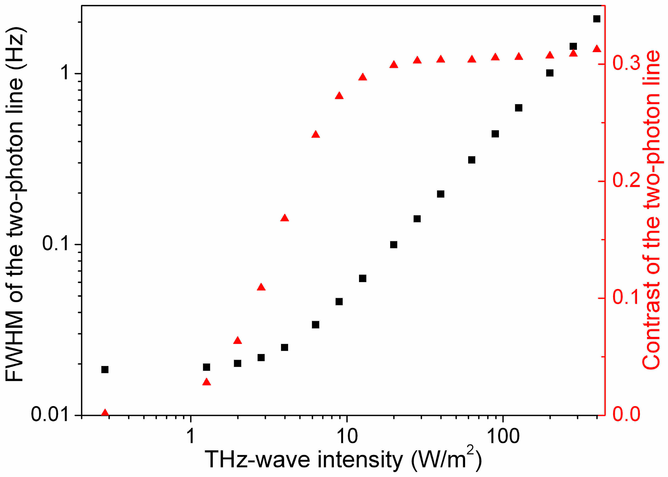
The linewidth of the two-photon rotational line is determined by power broadening. Figure 5 displays the dependence of the broadening in function of the THz-wave power (left-axis). The calculated linewidth decreases linearly with the THz-wave power before stabilizing at a level determined by the natural linewidth of the transition. The dependence of the contrast of the two-photon rotational line is shown on the right-axis. The offset remains stable when the THz-wave power varies. A lower THz-wave power may be used to increase the resolution of the two-photon line at the expense of the reduction of its contrast.
This two-photon spectroscopy scheme may be extended to other vibrational energy levels. Some two-photon rovibrational transitions have been identified between v = 0 and v′ = 2 and between v = 0 and v′ = 4 for L, L′ ≤ 5, respectively [30]. The HD+ ions in the v = 2 level require excitation to another vibrational level before dissociation. The HD+ ions in the v = 4 level can be efficiently dissociated with a 266 nm laser.
4. Perspectives in Stability and Accuracy from Two-Photon Rotational Transitions
The stability of a molecular clock based on the transitions of HD+ constrains the integration time required to determine the fundamental constants at a given level of statistical uncertainty. When the quantum projection noise dominates among other sources of noise, the stability is given by [31]:
The quality factor of the two-photon transition Q = ω2ph/ΔωHWHM is expressed in terms of the half-linewidth determined ultimately by the natural lifetimes of the molecular levels. The cycle time Tc is associated to a single measurement with Nion ions at two-photon resonance and successive measurements are averaged during an interrogation time τ > Tc. The two-photon transitions between the rotational levels with L < 5 in the vibrational ground state are more interesting because they display lifetimes which are ~102–103 greater than those of the two-photon rovibrational transitions to v > 4 levels [28]. Using the two-photon transition rate lineshape and supposing that the same number of ions are detected during the same measurement times, it appears that a molecular clock based on the fundamental two-photon rotational transition (v,L) = (0,0)→(0,2) may improve the stability by an order of magnitude compared to the stability reached by using the two-photon rovibrational transition (v,L) = (0,3)→(9,3) [20]. For example, using a cycle time of Tc = 2 s, the stability of a single-ion HD+ clock based on the rotational transition (v,L) = (0,1)→(0,3) is estimated at σy(τ) = 1.4 × 10⁻¹⁵τ−1/2, which is comparable with the stability of the optical atomic clocks based on trapped ions [31].
The higher resolution allowed by two-photon rotational spectroscopy opens the way to address individual Zeeman components of hyperfine structure energy levels. For the levels in the vibrational ground state with the same (F,S,J), the increase of L is associated generally to a decrease of Zeeman shift coefficients [25]. For metrological applications, it is interesting to select transitions with minimal Zeeman shifts as was suggested in [25,32]:
- -
- Transitions ππ between Jz = 0→J′z = 0 states that have only quadratic Zeeman shift.
- -
- Transitions σ±σ± between “stretched states”, that are pure eigenvectors of the angular momentum coupling with maximum total angular momentum and projection on the quantisation axis |v,L,F = 1,S = 2,J = L + 2,Jz = ±(L + 2)>, for which the Zeeman shifts depend linearly with the magnetic field, have the same magnitude but opposite values.
Zeeman shift coefficients are calculated for hyperfine components of rotational transitions using the polynomial expansion of the Zeeman shift of the energy levels from [25]. Transitions with small Zeeman shifts are shown in Table 3. The transition (v = 0,L = 1,F = 0,S = 1,J = 1,Jz = 0)→(v’ = 0,L’ = 3,F’ = 0,S’ = 1,J’ = 3,J’z = 0) benefits from a strong cancellation of the quadratic Zeeman shifts of the upper and lower levels. Assuming conservatively that the uncertainty is given by the Zeeman shift, estimated at 71.2 mHz for a value of the magnetic field of B = 0.02 G, the accuracy is 2.2 × 10⁻¹⁴. The Zeeman shift coefficients for two-photon rotational transitions between stretched states increase with L. The transition (v = 0,L = 0,F = 1,S = 2,J = 2,Jz = 2)→(v’ = 0,L’ = 2,F’ = 1,S’ = 2,J’ = 4,J’z = 4) benefits from the compensation between the linear Zeeman coefficients in the upper and lower levels. The Zeeman shift, estimated at −11.12 Hz for a value of the magnetic field of B = 0.02 G, leads to an accuracy of 5.6 × 10⁻¹².
A cancellation procedure was proposed for the linear Zeeman shift with pairs of transitions Jz→Jz and −Jz→−Jz [16] or for the Zeeman shift with pairs of transitions between stretched states Jz = ±(L + 2)→J’z = ±(L′ + 2) [16,25]. The idea was to calculate the mean frequency of such a pair of Zeeman-shifted hyperfine components. Consider here that each linecenter is determined within 1% of an experimental linewidth that is taken at 1 Hz. The uncertainty of the determination of the average frequency is 0.01 × Hz, that may be improved by a factor of 10 by doing the linear regression of the dependence of the frequency splitting on the magnetic field. The estimated accuracy is 4.3 × 10⁻¹⁶ for hyperfine components of the (v,L) = (0,1)→(0,3) two-photon rotational transition.
The dynamic polarisabilities for the selected hyperfine levels coupled by two-photon rotational transitions are determined with Equations (17)–(19) and displayed in Table 3. The polarisabilities in the upper and lower levels are efficiently compensated for many hyperfine components of Jz = 0→J′z = 0 transitions. The lightshifts are estimated for a THz-wave intensity of 1 mW/mm2. The accuracies are ≤ 2 × 10⁻¹³ and a value of 4 × 10⁻¹⁵ is reached for the (v = 0,L = 1,F = 0,S = 1,J = 2,Jz = 0)→(v’ = 0,L’ = 3,F’ = 0,S’ = 1,J’ = 4,J’z = 0) transition.
A method for the reduction of the lightshift, suggested in [20], exploits two lasers with suitable power to probe the two-photon transition in the Lamb-Dicke regime. Alternatively, the interaction with sequences of suitably tailored laser pulses may provide a dramatic reduction of the lightshifts, as was suggested in a generalisation of the Ramsey spectroscopy method [33]. A hyper-Ramsey scheme was successfully implemented on the octupole clock transition of a single trapped 171Yb+ ion leading to the reduction of the lightshift by orders of magnitude below to the 10−16 level [34]. An approach was recently proposed for Doppler-free optical stimulated Raman transitions [35].
5. Determination of Fundamental Constants
The comparison of experimental frequencies of HD+ ions transitions with accurate theoretical predictions is used here to determine independent values for fundamental constants. This section follows the approach of CODATA least-squares adjustment [36] that has been exploited with hydrogen molecular ion rovibrational transitions [37].
The energy levels of HD+ ions may be calculated in the frameworks of QED and quantum chromodynamics (QCD) as a series expansion:
in function of the Rydberg constant R∞, the proton-to-electron mass ratio µpe = Mp/me, the deuteron-to-proton mass ratio µdp = Md/Mp, the fine-structure constant α, the proton radius rp, the deuteron radius rd, and the Bohr radius a0 = α/4πR∞. The first term Enr is the non-relativistic energy given by the Schrödinger equation. The next term is a series expansion of corrections to the energy levels in terms of α (QED corrections), Zp,dα (relativistic corrections), and me/Mp,d (recoil corrections). The last term is a correction from QCD associated to the finite-size of the proton and the deuteron. Corrections of orders up to meα8 to HD+ energy levels were calculated in [8,9,10,11,38,39].
The sensitivity coefficient of a transition to a constant c is expressed as:
Here, f0 is the HD+ ion transition frequency calculated with the set of the recommended values of fundamental constants {c0} given by CODATA 2014 [1]. Sensitivity coefficients for selected two-photon HD+ ion transitions are calculated and presented in Table 4. The contribution from the non-relativistic energy is accounted for with the values of ∂E/∂ln(µpe,dp) calculated in [23]. The recoil corrections bring a negligible fractional contribution to the sensitivity coefficients to the nuclear-to-electron mass ratios. Sensitivity to α is not addressed here and the sensitivity coefficients to R∞ may be taken as 1 for simplicity. The rotational transitions have sensitivity coefficients to the relevant constants by a factor of two higher than the corresponding sensitivity coefficients of the vibrational transitions.
Fundamental constants are extracted with an uncertainty that depends on the accuracy of the experimental frequencies and the accuracy of the predictions. The experimental accuracy for all two-photon rovibrational transitions is assumed here to be 10−12 as in [20]. The estimation is based on linewidths ~500 Hz, determined by the spectral purity of the laser and power broadening and by the signal-to-noise ratio of an rovibrational signal of an experiment [17]. The estimated uncertainty is, therefore, one tenth of the linewidth. It is assumed here that all two-photon rotational transitions may be observed with the same noise and with linewidths ~1 Hz determined by power broadening. Each two-photon rotational transition requires an extremely narrow THz source and provides a signal smaller than the signal from the corresponding two-photon rovibrational transition. The uncertainty for all two-photon rotational transitions is conservatively estimated here at one half of the linewidth and the accuracy is assumed at 5 × 10⁻¹³. The uncertainties of the experimental frequencies due to various systematic effects are supposed to be below the estimated experimental accuracies. Calculations with corrections to order meα7 predicted HD+ ion frequencies with an accuracy estimated at 3–4 × 10⁻¹¹ [10]. The inclusion of other corrections may improve the value of the theoretical uncertainty [37] that is assumed here at 3 × 10⁻¹² for all transitions. In the least squares method, the dependence of the transition frequencies on the adjusted constants is linearized using a Taylor expansion around the starting values of the constants. The dependence is expressed with the matrix relation Y = AX, where Y = {y1,y2,…,yN1}, with yi = (fi− fi,0)/fi,0, and X = {x1,x2,…,xN2}, with xj = (cj− cj,0)/cj,0, are columns with N1,2 elements respectively. The sensitivity matrix A is a N1 × N2 matrix with elements aij = d(lnf0,i)/d(lnc0,j). The covariance matrix of the solution X is expressed in terms of the covariance matrix of the input data V and the sensitivity matrix as:
The uncertainty of the input data is taken as the root-mean-square sum of the experimental and theoretical uncertainties. The covariances of the input data are given by the covariances of the predictions, by assuming that experimental frequencies are not correlated. Non-zero covariance arises from the uncalculated terms in the energy levels that are expressed as a particular constant multiplied by the common factor arising, for example, from the overlapping of the electron wavefunction with the extended nuclear charge distribution. A value of 1 for all correlation coefficients is taken here.
It is interesting to estimate the contributions to the theoretical uncertainty arising from the uncertainty of each fundamental constant. Using CODATA 2014 values and uncertainties of fundamental constants [1], the uncertainty propagation law yields for the transition (v,L) = (0,1)→(0,3) of HD+ the following values: [Δy(R∞),Δy(μpe),Δy(μdp),Δy(rp),Δy(rd)] = [0.59,9.4,3.1,0.74,0.76] × 10−11 (correlations between fundamental constants are not taken in account in this estimation). CODATA value of the proton-to-electron mass ratio is the main source of uncertainty. Discrepancies were noticed between CODATA values of rp and rd and the values inferred from muonic hydrogen [40] and from muonic deuterium [41]. The main disagreement concerns rp, and it may be judicious here to account for it by using an increased uncertainty Δx(rp) = 3.9 × 10⁻² that is equal to the difference between the rp values from the CODATA 2014 adjustment and the muonic hydrogen spectroscopy. The uncertainties for R∞ and rd have to be increased in proportion because of high correlation coefficients r(R∞,rp) = 0.9891 and r(rp,rd) = 0.9994, respectively [42]. The uncertainties for the rotational transition are now: [Δy(R∞),Δy(μpe),Δy(μdp),Δy(rp),Δy(rd)] = [3.3,9.4,3.1,4.1,4.2] × 10−11. The proton-to-electron mass ratio remains the main source of uncertainty, and the other constants bring contributions that are two or three times less.
Different combinations of transitions of H2+ and HD+ are tested in the least squares method and the uncertainties of the determination of fundamental constants are calculated. The results are displayed in Table 5. The values of five constants (R∞, μpe, μdp, rp, rd) may be derived independently of previous results from an adjustment of eight transitions (line B in Table 5). The accuracy of the proton-to-electron mass ratio is improved by one order of magnitude compared to the CODATA 2014 value, and the accuracy of the deuteron-to-proton mass ratio is improved by nearly a factor of 20. The accuracies of R∞, rp, and rd are comparable with the relevant values given by CODATA 2014. This adjustment may add clues to the proton radius puzzle, as the uncertainties for rp and rd are smaller than the corresponding discrepancies [2]. If the proton radius puzzle is solved and rp, rd can be precisely determined by atomic spectroscopy of muonic hydrogen and muonic deuterium, respectively, three constants (R∞, μpe, μdp) can be determined using an adjustment of four transitions (line C in Table 5). The accuracies are improved by factors of (1.8, 25, 11) compared to the relevant CODATA 2014 values. Finally, if R∞, rp, and rd may be determined accurately by atomic spectroscopy, one could address again the starting point of hydrogen molecular ions spectroscopy that is accurate nuclear-to-electron mass ratio determination. Using an adjustment of three transitions (line D in Table 5), the proton-to-electron mass ratio and the deuteron-to-proton mass ratio may be determined with accuracies improved by factors of 26 and 12 compared to the relevant values given by CODATA 2014. Note that using in addition a two-photon rotational transition in the adjustment improves the accuracy by more than a factor of 1.5 compared to the result from [37] with solely rovibrational data. Moreover, accurate values of the mass ratios µrp and µdp may be associated with the new value of the electron mass [43], determined with an accuracy of 3 × 10⁻¹¹ from a measurement of the g-factor, to improve the determination of the proton and the deuteron relative masses.
6. Conclusions
This contribution demonstrates the potential of two-photon rotational and rovibrational transitions probed on trapped HD+ for the determination of fundamental constants. The approach may provide an independent and accurate determination of the Rydberg constant and of the nuclear-to-electron mass ratios and may add new results to the efforts made to measure the size of the proton and of the deuteron. Measurements may be performed using a double resonance two-photon spectroscopy scheme. The lightshifts and the Zeeman shifts, calculated for several hyperfine components of the rotational transition, are beyond the 10−12 level. The experimental accuracy is estimated at the 10−12 level for the Doppler-free rotational and rovibrational transitions, while the theoretical calculations have the same level of accuracy. Depending on possible issues of the proton radius puzzle in atomic spectroscopy, HD+ ion two-photon spectroscopy may improve the determination of the proton-to-electron and deuteron-to-proton mass ratios beyond the 10−11 level. The comparison between the values of fundamental constants determined from HD+ ion spectroscopy and from CODATA adjustment may allow a test of consistency of QED calculations and precision measurements for different physical systems.
Conflicts of Interest
The author declares no conflict of interest.
References
- Mohr, P.J.; Taylor, B.N.; Newell, D.B. CODATA recommended values of the fundamental physical constants: 2014. Rev. Mod. Phys. 2014, 88, 1527–1605. [Google Scholar] [CrossRef]
- Pohl, R.; Nez, F.; Udem, T.; Antognini, A.; Beyer, A.; Fleurbaey, H.; Grinin, A.; Hänsch, T.W.; Julien, L.; Kottmann, F.; et al. Deuteron charge radius and Rydberg constant from spectroscopy data in atomic deuterium. Metrologia 2017, 54, L1–L10. [Google Scholar] [CrossRef]
- Richard, J.H. Review of experimental and theoretical status of the proton radius puzzle. EPJ Web Conf. 2017, 137, 01023. [Google Scholar] [CrossRef]
- Uzan, J.-P. The fundamental constants and their variation: Observational and theoretical status. Rev. Mod. Phys. 2003, 75, 403–455. [Google Scholar] [CrossRef]
- Jansen, P.; Bethlem, H.L.; Ubachs, W. Perspective: Tipping the scales: Search for drifting constants from molecular spectra. J. Chem. Phys. 2014, 140, 010901. [Google Scholar] [CrossRef] [PubMed]
- Carrington, A.; McNab, I.R.; Montgomerie, C.A. Spectroscopy of the hydrogen molecular ion. J. Phys. B 1989, 22, 3551–3586. [Google Scholar] [CrossRef]
- Roth, B.; Koelemeij, J.; Schiller, S.; Hilico, L.; Karr, J.-P.; Korobov, V.I.; Bakalov, D. Precision spectroscopy of molecular hydrogen ions: towards frequency metrology of particle masses. In Precision Physics of Simple Atoms and Molecules; Karshenboim, S., Ed.; Lectures Notes in Physics; Springer: Berlin/Heidelberg, Germany, 2008; Volume 745, pp. 205–232. ISBN 978-3-540-75478-7. [Google Scholar]
- Korobov, V.I. Relativistic corrections of mα6 order to the rovibrational spectrum of H2+ and HD+ molecular ions. Phys. Rev. A 2008, 77, 022509. [Google Scholar] [CrossRef]
- Korobov, V.I.; Hilico, L.; Karr, J.-P. Theoretical transition frequencies beyond 0.1 p.p.b. accuracy in H2+, HD+, and antiprotonic helium. Phys. Rev. A 2014, 89, 032511. [Google Scholar] [CrossRef]
- Korobov, V.I.; Hilico, L.; Karr, J.-P. mα7-Order corrections in the hydrogen molecular ions and antiprotonic helium. Phys. Rev. Lett. 2014, 112, 103003. [Google Scholar] [CrossRef] [PubMed]
- Korobov, V.I.; Hilico, L.; Karr, J.-P. Fundamental transitions and ionization energies of the hydrogen molecular ions with few ppt uncertainty. Phys. Rev. Lett. 2017, 118, 233001. [Google Scholar] [CrossRef] [PubMed]
- Staanum, P.F.; Hojbjerre, K.; Skyt, P.S.; Hansen, A.K.; Drewsen, M. Rotational laser cooling of vibrationally and translationally cold molecular ions. Nat. Phys. 2010, 6, 271–274. [Google Scholar] [CrossRef]
- Schneider, T.; Roth, B.; Duncker, H.; Ernsting, I.; Schiller, S. All-optical preparation of molecular ions in the rovibrational ground state. Nat. Phys. 2010, 6, 275–278. [Google Scholar] [CrossRef]
- Peek, J.M.; Hashemi-Attar, A.-R.; Beckel, C.L. Spontaneous emission lifetimes in the ground electronic states of HD+ and H2+. J. Chem. Phys. 1979, 71, 5382–5383. [Google Scholar] [CrossRef]
- Karr, J.-P. H2 + and HD+: Candidates for a molecular clock. J. Mol. Spectrosc. 2014, 300, 37–43. [Google Scholar] [CrossRef]
- Schiller, S.; Bakalov, D.; Korobov, V.I. Simplest molecules as candidates for precise optical clocks. Phys. Rev. Lett. 2014, 113, 023004. [Google Scholar] [CrossRef] [PubMed]
- Biesheuvel, J.; Karr, J.-P.; Hilico, L.; Eikema, K.S.E.; Ubachs, W.; Koelemeij, J.C.J. Probing QED and fundamental constants through laser spectroscopy of vibrational transitions in HD+. Nat. Commun. 2016, 7, 10385. [Google Scholar] [CrossRef] [PubMed]
- Wing, W.H.; Ruff, G.A.; Lamb, W.E., Jr.; Spezeski, J.J. Observation of the infrared spectrum of the hydrogen molecular ion HD+. Phys. Rev. Lett. 1976, 36, 1488–1491. [Google Scholar] [CrossRef]
- Salumbides, E.J.; Koelemeij, J.C.J.; Komasa, J.; Pachucki, K.; Eikema, K.S.E.; Ubachs, W. Bounds on fifth forces from precision measurements on molecules. Phys. Rev. D 2013, 87, 112008. [Google Scholar] [CrossRef]
- Tran, V.Q.; Karr, J.-P.; Douillet, A.; Koelemeij, J.C.J.; Hilico, L. Two-photon spectroscopy of trapped HD+ ions in the Lamb-Dicke regime. Phys. Rev. A 2013, 88, 033421. [Google Scholar] [CrossRef]
- Germann, M.; Tong, X.; Willitsch, S. Observation of electric-dipole-forbidden infrared transitions in cold molecular ions. Nat. Phys. 2014, 10, 820–824. [Google Scholar] [CrossRef]
- Cagnac, B.; Grynberg, G.; Biraben, F. Spectroscopie d’absorption multiphotonique sans effet Doppler. J. Phys. 1973, 34, 845–858. [Google Scholar] [CrossRef]
- Schiller, S.; Korobov, V. Tests of time independence of the electron and nuclear masses with ultracold molecules. Phys. Rev. A 2005, 71, 032505. [Google Scholar] [CrossRef]
- Bakalov, D.; Korobov, V.I.; Schiller, S. High-precision calculation of the hyperfine structure of the HD+ ion. Phys. Rev. Lett. 2006, 97, 243001. [Google Scholar] [CrossRef] [PubMed]
- Bakalov, D.; Korobov, V.I.; Schiller, S. Magnetic field effects in the transitions of the HD+ molecular ion and precision spectroscopy. J. Phys. B 2011, 44, 025003. [Google Scholar] [CrossRef]
- Brown, J.; Carrington, A. Rotational Spectroscopy of Diatomic Molecules, 1st ed.; Cambridge University Press: Cambridge, UK, 2003; ISBN 0-521-53078-4. [Google Scholar]
- Bakalov, D.; Schiller, S. Static Stark effect in the molecular ion HD+. Hyperfine Interact. 2012, 210, 25–31. [Google Scholar] [CrossRef]
- Amitay, Z.; Zajfman, D.; Forck, P. Rotational and vibrational lifetime of isotopically asymmetrized homonuclear diatomic molecular ions. Phys. Rev. A 1994, 50, 2304–2308. [Google Scholar] [CrossRef] [PubMed]
- Constantin, F.L. Feasibility of two-photon rotational spectroscopy on trapped HD+. In Proceedings of the SPIE Photonics Europe, Brussels, Belgium, 3–7 April 2016. [Google Scholar]
- Karr, J.-P.; Kilic, S.; Hilico, L. Energy levels and two-photon transition probabilities in the HD+ ion. J. Phys. B 2005, 38, 853–866. [Google Scholar] [CrossRef]
- Margolis, H.S. Frequency metrology and clocks. J. Phys. B 2009, 42, 154017. [Google Scholar] [CrossRef]
- Bakalov, D.; Schiller, S. The electric quadrupole moment of molecular hydrogen ions and their potential for a molecular ion clock. Appl. Phys. B 2014, 114, 213–230. [Google Scholar] [CrossRef]
- Yudin, V.I.; Taichenachev, A.V.; Oates, C.W.; Barber, Z.W.; Lemke, N.D.; Ludlow, A.D.; Sterr, U.; Lisdat, Ch.; Riehle, F. Hyper-Ramsey spectroscopy of optical clock transitions. Phys. Rev. A 2010, 82, 011804. [Google Scholar] [CrossRef]
- Huntemann, N.; Lipphardt, B.; Okhapkin, M.; Tamm, Chr.; Peik, E.; Taichenachev, A.V.; Yudin, V.I. Generalized Ramsey excitation scheme with suppressed light shift. Phys. Rev. Lett. 2012, 109, 213002. [Google Scholar] [CrossRef] [PubMed]
- Zanon-Willette, T.; Almonacil, S.; de Clercq, E.; Ludlow, A.D.; Arimondo, E. Quantum engineering of atomic phase shifts in optical clocks. Phys. Rev. A 2014, 90, 053427. [Google Scholar] [CrossRef]
- Mohr, P.J.; Taylor, B.N. CODATA recommended values of the fundamental physical constants: 1998. Rev. Mod. Phys. 2000, 72, 351–495. [Google Scholar] [CrossRef]
- Karr, J.-P.; Hilico, L.; Koelemeij, J.C.J.; Korobov, V.I. Hydrogen molecular ions for improved determination of fundamental constants. Phys. Rev. A 2016, 94, 050501. [Google Scholar] [CrossRef]
- Korobov, V.I. Bethe logarithm for the hydrogen molecular ion HD+. Phys. Rev. A 2004, 70, 012505. [Google Scholar] [CrossRef]
- Korobov, V.I. Leading-order relativistic and radiative corrections to the rovibrational spectrum of H2+ and HD+. Phys. Rev. A 2005, 74, 052506. [Google Scholar] [CrossRef]
- Antognini, A.; Nez, F.; Schuhmann, K.; Amaro, F.D.; Biraben, F.; Cardoso, J.M.R.; Covita, D.S.; Dax, A.; Dhawan, S.; Diepold, M.; et al. Proton structure from the measurement of 2S-2P transition frequencies of muonic hydrogen. Science 2013, 339, 417–420. [Google Scholar] [CrossRef] [PubMed]
- Pohl, R.; Nez, F.; Fernandes, L.M.P.; Amaro, F.D.; Biraben, F.; Cardoso, J.M.R.; Covita, D.S.; Dax, A.; Dhawan, S.; Diepold, M.; et al. Laser spectroscopy of muonic deuterium. Science 2016, 353, 669–673. [Google Scholar] [CrossRef] [PubMed]
- Taylor, B.N.; Mohr, P.J. The NIST Reference on Constants, Units, and Uncertainty. Available online: https://physics.nist.gov/cuu/Constants/index.html (accessed on 26 August 2017).
- Sturm, S.; Köhler, S.; Zatorski, J.; Wagner, A.; Harman, Z.; Werth, G.; Quint, W.; Keitel, C.H.; Blaum, K. High-precision measurement of the atomic mass of the electron. Nature 2014, 506, 467–470. [Google Scholar] [CrossRef] [PubMed]
Figure 1.
Average of the squared two-photon reduced matrix elements for ππ excitation between the rotational levels (v = 0,L = 1) and (v = 0,L = 3), in atomic units. The spectrum is centred on the hyperfine-free rotational frequency given in Table 1.
Figure 1.
Average of the squared two-photon reduced matrix elements for ππ excitation between the rotational levels (v = 0,L = 1) and (v = 0,L = 3), in atomic units. The spectrum is centred on the hyperfine-free rotational frequency given in Table 1.
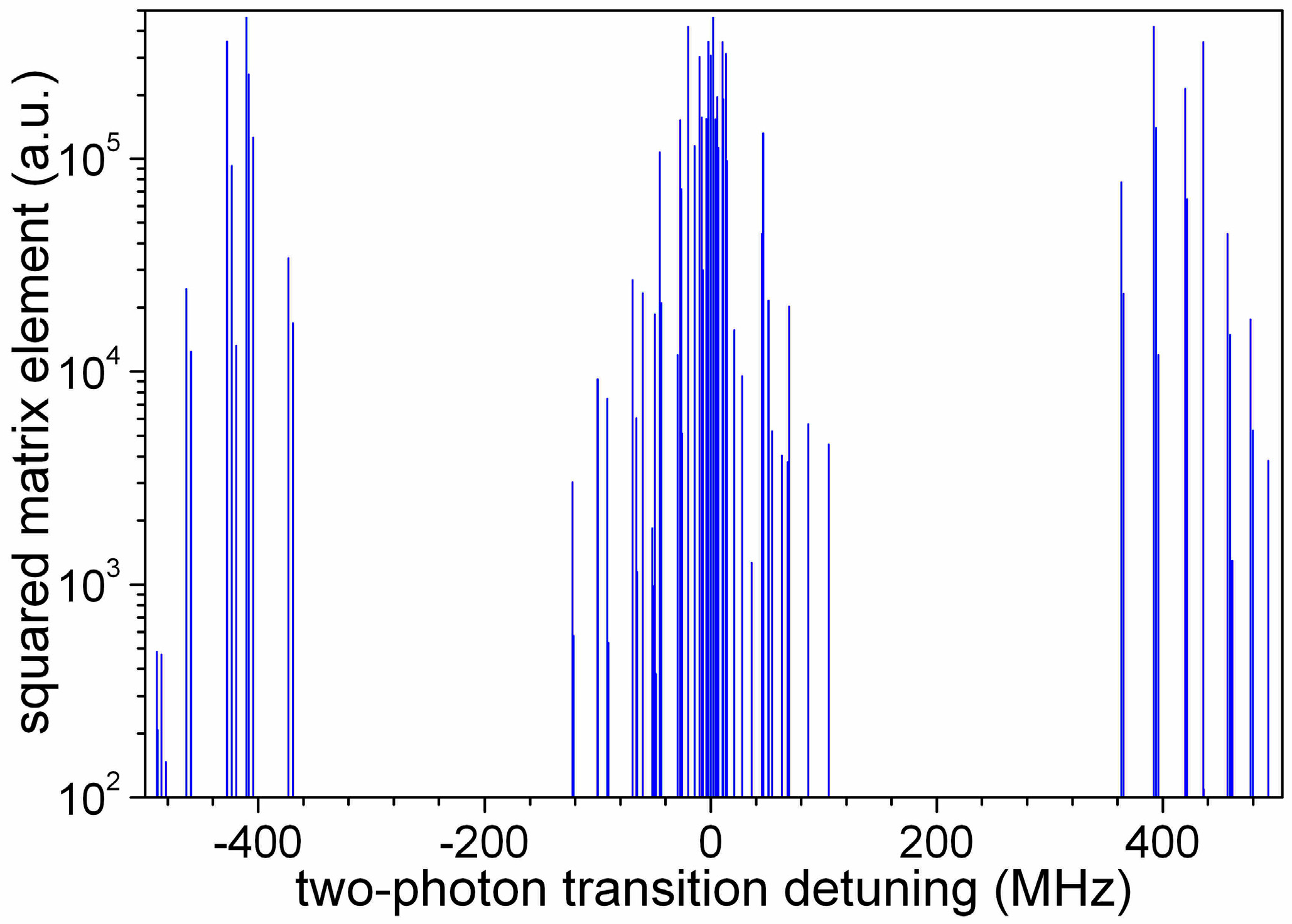
Figure 2.
The closed set of energy levels addressed by the THz/infrared double resonance two-photon spectroscopy scheme mediated by the blackbody radiation.
Figure 2.
The closed set of energy levels addressed by the THz/infrared double resonance two-photon spectroscopy scheme mediated by the blackbody radiation.
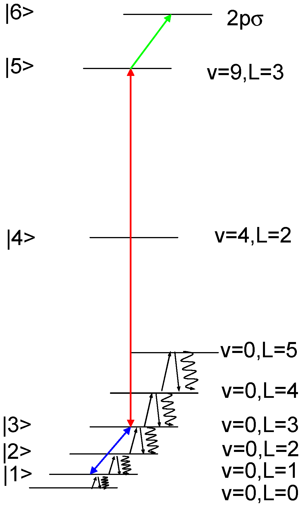
Figure 3.
Time dependences of the populations in selected rovibrational levels (continuous lines, left-axis) upon two-photon rotational excitation (v,L) = (0,1)→(0,3), two-photon rovibrational excitation (v,L) = (0,3)→(9,3), and dissociation (v,L) = (9,3)→2pσ. Time dependence of the fractional population in the (v,L) = (0,0) level (red dotted curve, right-axis). Values assumed for the transition rates when the lasers are tuned at resonance: Γ2ph,r = 2000 s−1 (ITHz = 1 mW/mm2), Γ2ph,r = 10 s−1 (IIR ~ 5 mW/mm2), Γdiss = 200 s−1 (Ivis = 56 mW/mm2).
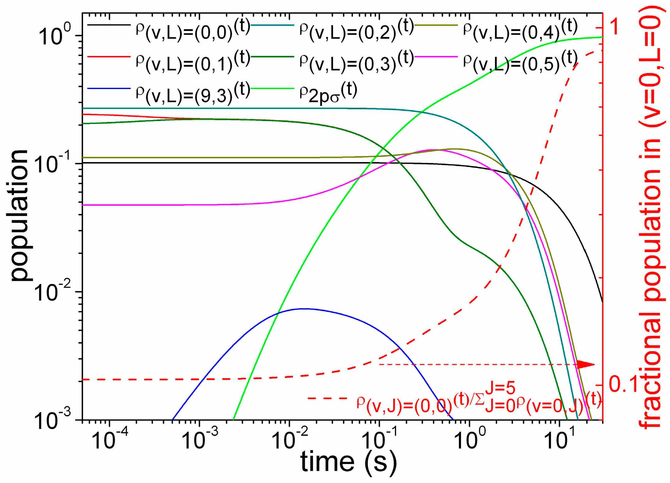
Figure 4.
(a) Spectra of the two-photon rovibrational transition calculated with (green continuous line) or without (blue dotted line) THz-wave tuned at the two-photon rotational resonance. (b) Spectrum of the two-photon rotational transition (red continuous line) at the two-photon rovibrational resonance.
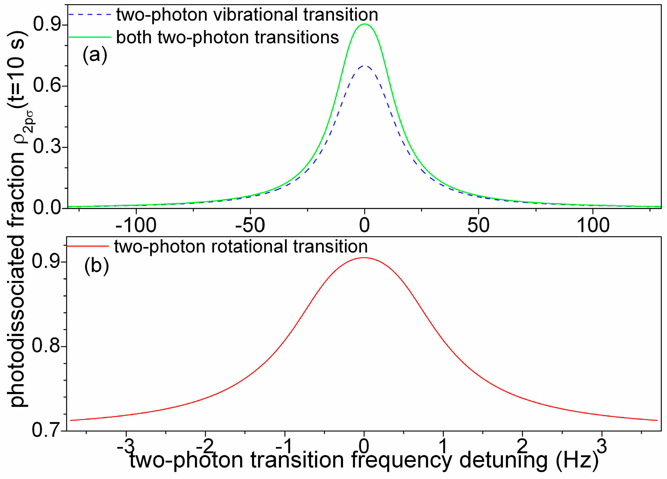
Figure 5.
Dependence of the FWHM linewidth of the two-photon rotational line on the THz-wave power (black squares, left-axis). Dependence of the contrast of the two-photon rotational line with the THz-wave power (red triangles, right-axis).
Figure 5.
Dependence of the FWHM linewidth of the two-photon rotational line on the THz-wave power (black squares, left-axis). Dependence of the contrast of the two-photon rotational line with the THz-wave power (red triangles, right-axis).

Table 1.
Reduced matrix elements of the operator Q(2) for the transitions (v = 0,L)→(v′ = 0,L′ = L + 2) with 0 ≤ L ≤ 3, in atomic units.
Table 1.
Reduced matrix elements of the operator Q(2) for the transitions (v = 0,L)→(v′ = 0,L′ = L + 2) with 0 ≤ L ≤ 3, in atomic units.
| v | L | v′ | L′ | Frequency (THz) | Q(2) (a.u.) |
|---|---|---|---|---|---|
| 0 | 0 | 0 | 2 | 1.968 | 1367.669 |
| 0 | 1 | 0 | 3 | 3.268 | −3228.723 |
| 0 | 2 | 0 | 4 | 4.548 | 5589.249 |
| 0 | 3 | 0 | 5 | 5.801 | −8478.534 |
Table 2.
Reduced matrix elements of the two-photon operator Q(k)(EvL±ω) for the transitions (v = 0,L)→(v′ = 0,L′ = L + 2) with 0 ≤ L ≤ 3, in atomic units.
Table 2.
Reduced matrix elements of the two-photon operator Q(k)(EvL±ω) for the transitions (v = 0,L)→(v′ = 0,L′ = L + 2) with 0 ≤ L ≤ 3, in atomic units.
| v | L | v′ | L′ | Q(0)(Ev,L + ω)(a.u.) | Q(2)(Ev,L + ω)(a.u.) | Q(0)(Ev′,L′ + ω)(a.u.) | Q(2)(Ev′,L′ + ω)(a.u.) |
| 0 | 0 | 0 | 2 | 682.990 | 0 | −756.843 | −121.457 |
| 0 | 1 | 0 | 3 | 1656.527 | 483.476 | −1218.221 | −420.161 |
| 0 | 2 | 0 | 4 | 2965.652 | 1226.224 | −1785.156 | −780.275 |
| 0 | 3 | 0 | 5 | 4578.742 | 2190.257 | −2470.049 | −1216.183 |
| v | L | v′ | L′ | Q(0)(Ev,L − ω)(a.u.) | Q(2)(Ev,L − ω)(a.u.) | Q(0)(Ev′,L′ − ω)(a.u.) | Q(2)(Ev′,L′ − ω)(a.u.) |
| 0 | 0 | 0 | 2 | −136.031 | 0 | 916.768 | 1503.824 |
| 0 | 1 | 0 | 3 | −307.656 | −334.504 | 2044.727 | 2447.167 |
| 0 | 2 | 0 | 4 | −630.082 | −631.130 | 3459.700 | 3597.655 |
| 0 | 3 | 0 | 5 | −1060.515 | −1002.231 | 5184.501 | 4973.626 |
Table 3.
Selected hyperfine components of two-photon rotational transitions and estimations of systematic effects. Zeeman shift coefficients ΔηB2, ΔηB for transitions between (a) Jz = J′z = 0 states, (b) stretched states. Polarisabilities α, α′ in atomic units and lightshift coefficients ΔηLS.
Table 3.
Selected hyperfine components of two-photon rotational transitions and estimations of systematic effects. Zeeman shift coefficients ΔηB2, ΔηB for transitions between (a) Jz = J′z = 0 states, (b) stretched states. Polarisabilities α, α′ in atomic units and lightshift coefficients ΔηLS.
| (a) | |||||
| v,L,F,S,J;Jz | v′,L′,F′,S′,J′;J′z | ΔηB2 (Hz/G2) | α (a.u.) | α′ (a.u.) | ΔηLS (Hz/(W/cm2)) |
| 0,0,0,1,1;0 | 0,2,0,1,3;0 | −1062 | 315.787 | 257.141 | 1.374 |
| 0,0,1,0,0;0 | 0,2,1,0,2;0 | 3100 | 315.787 | 311.103 | 0.110 |
| 0,1,0,1,0;0 | 0,3,0,1,2;0 | −841.5 | 449.624 | 457.242 | −0.179 |
| 0,1,0,1,1;0 | 0,3,0,1,3;0 | 178 | 427.416 | 422.632 | 0.112 |
| 0,1,0,1,2;0 | 0,3,0,1,4;0 | 641.5 | 471.831 | 468.779 | 0.072 |
| 0,1,1,0,1;0 | 0,3,1,0,3;0 | 1356 | 494.038 | 503.390 | −0.219 |
| 0,1,1,1,2;0 | 0,3,1,1,4;0 | −1426.5 | 471.831 | 468.779 | 0.072 |
| 0,1,1,2,1;0 | 0,3,1,2,3;0 | 2019 | 454.065 | 282.652 | 4.017 |
| (b) | |||||
| v,L,F,S,J;Jz | v′,L′,F′,S′,J′;J′z | ΔηB (Hz/G) | α (a.u.) | α′ (a.u.) | ΔηLS (Hz/(W/cm2)) |
| 0,0,1,2,2;2 | 0,2,1,2,4;4 | −556 | −315.787 | −176.198 | −3.271 |
| 0,1,1,2,3;3 | 0,3,1,2,5;5 | −2278 | −460.727 | −382.253 | −1.839 |
| 0,2,1,2,4;4 | 0,4,1,2,6,6 | −24,747 | −661.117 | −595.822 | −1.530 |
Table 4.
Selected rotational and rovibrational two-photon transitions of HD+ and H2+: frequencies and sensitivity coefficients to constants used in adjustments. Data for H2+ is taken from [37].
Table 4.
Selected rotational and rovibrational two-photon transitions of HD+ and H2+: frequencies and sensitivity coefficients to constants used in adjustments. Data for H2+ is taken from [37].
| Label | v | L | v′ | L′ | Freq. (THz) | Kµpe | Kµdp | 109 × Krp | 109 × Krd |
|---|---|---|---|---|---|---|---|---|---|
| HD[1] | 0 | 0 | 0 | 2 | 1.9685 | −0.9848 | −0.3284 | −1.0581 | −6.3355 |
| HD[2] | 0 | 1 | 0 | 3 | 3.2677 | −0.9808 | −0.3271 | −1.0547 | −6.3151 |
| HD[3] | 0 | 2 | 0 | 4 | 4.5477 | −0.9749 | −0.3251 | −1.0497 | −6.2848 |
| HD[4] | 0 | 1 | 2 | 1 | 55.8500 | −0.4601 | −0.1534 | −0.6192 | −3.7012 |
| HD[5] | 0 | 2 | 2 | 0 | 53.9407 | −0.4421 | −0.1474 | −0.6039 | −3.6095 |
| HD[6] | 0 | 3 | 2 | 1 | 52.5823 | −0.4277 | −0.1427 | −0.5922 | −3.5388 |
| HD[7] | 0 | 4 | 2 | 2 | 51.1844 | −0.4120 | −0.1374 | −0.5795 | −3.4626 |
| HD[8] | 0 | 4 | 4 | 4 | 105.0777 | −0.4235 | −0.1412 | −0.6040 | −3.6073 |
| HD[9] | 0 | 5 | 4 | 5 | 104.5129 | −0.4179 | −0.1394 | −0.6010 | −3.5870 |
| HD[10] | 0 | 3 | 9 | 3 | 207.6343 | −0.3522 | −0.1175 | −0.5880 | −3.5000 |
| H2[1] | 0 | 2 | 1 | 2 | 32.7293 | −0.4657 | 0 | −1.2400 | 0 |
| H2[2] | 3 | 2 | 4 | 2 | 27.1961 | −0.3652 | 0 | −1.1730 | 0 |
| H2[3] | 5 | 2 | 6 | 2 | 23.7417 | −0.2801 | 0 | −1.1330 | 0 |
| H2[4] | 6 | 2 | 7 | 2 | 22.0540 | −0.2279 | 0 | −1.1140 | 0 |
Table 5.
Estimation of the accuracy of the determination of fundamental constants from an adjustment of two-photon transitions of hydrogen molecular ions, that are referenced in Table 4. Line A gives the uncertainties of relevant fundamental constants from the CODATA 2014 adjustment. Lines B, C, and D give the uncertainties for the determination of the fundamental constants with the adjustments discussed in the text.
| Adjustment | Δx(R∞) × 1011 | Δx(μpe) × 1011 | Δx(μdp) × 1011 | Δx(rp) × 103 | Δx(rd) × 103 |
|---|---|---|---|---|---|
| A: CODATA | 0.59 | 9.5 | 9.3 | 7.0 | 1.2 |
| B: HD[1], HD[2], HD[4], HD[10], H2[1], H2[2], H2[3], H2[4] | 0.84 | 0.78 | 0.55 | 8.2 | 3.3 |
| C: HD[2], HD[10], H2[1], H2[4] | 0.33 | 0.38 | 0.83 | ||
| D: HD[2], HD[10], H2[1] | 0.37 | 0.80 |
© 2017 by the author. Licensee MDPI, Basel, Switzerland. This article is an open access article distributed under the terms and conditions of the Creative Commons Attribution (CC BY) license (http://creativecommons.org/licenses/by/4.0/).
Share and Cite
MDPI and ACS Style
Constantin, F.L. THz/Infrared Double Resonance Two-Photon Spectroscopy of HD+ for Determination of Fundamental Constants. Atoms 2017, 5, 38. https://doi.org/10.3390/atoms5040038
AMA Style
Constantin FL. THz/Infrared Double Resonance Two-Photon Spectroscopy of HD+ for Determination of Fundamental Constants. Atoms. 2017; 5(4):38. https://doi.org/10.3390/atoms5040038
Chicago/Turabian StyleConstantin, Florin Lucian. 2017. "THz/Infrared Double Resonance Two-Photon Spectroscopy of HD+ for Determination of Fundamental Constants" Atoms 5, no. 4: 38. https://doi.org/10.3390/atoms5040038
Note that from the first issue of 2016, this journal uses article numbers instead of page numbers. See further details here.