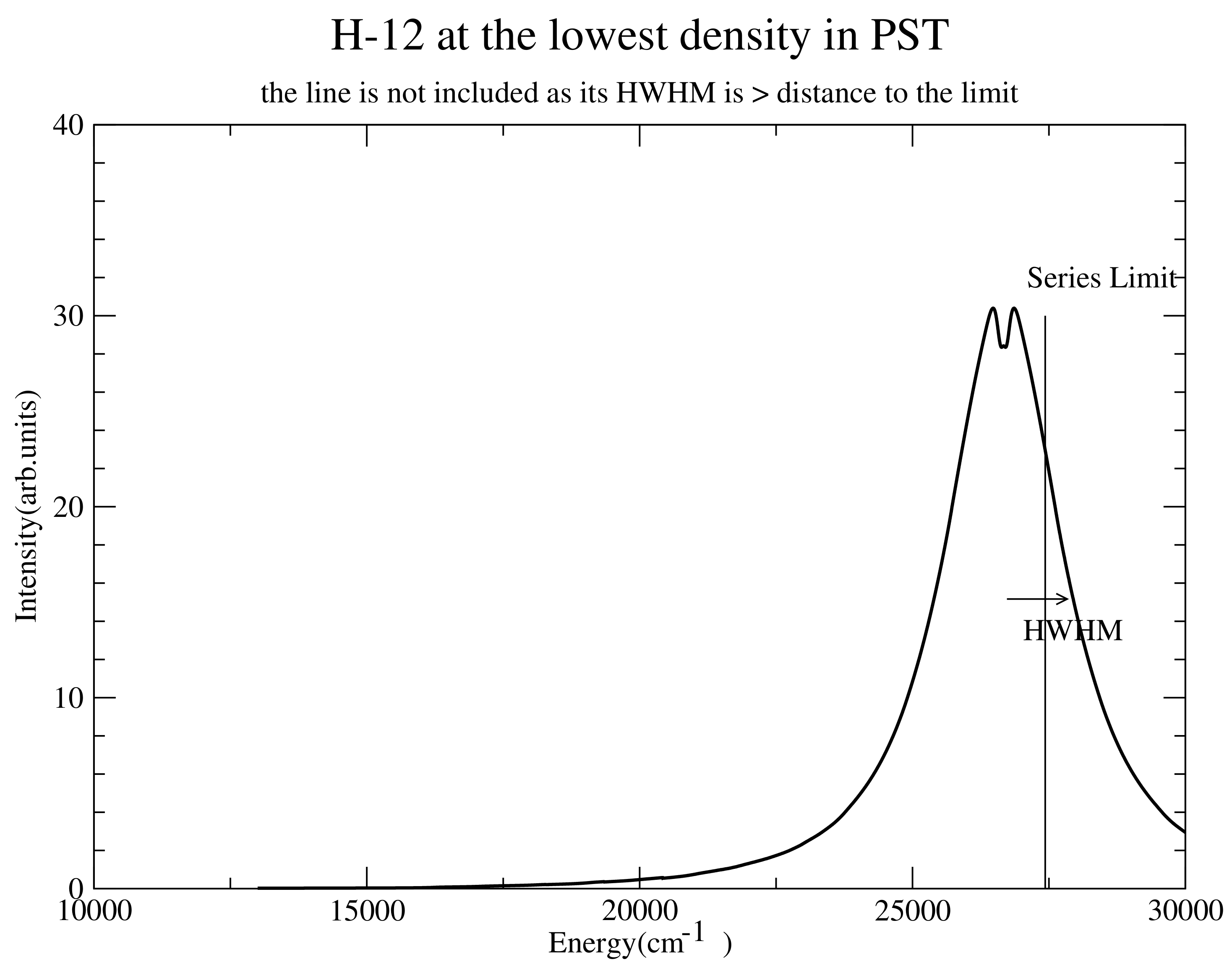
Figure 1.
computed with account of penetrating collisions (PST) at the lowest density considered showing a HWHM that is larger than the distance to the continuum.
Figure 1.
computed with account of penetrating collisions (PST) at the lowest density considered showing a HWHM that is larger than the distance to the continuum.
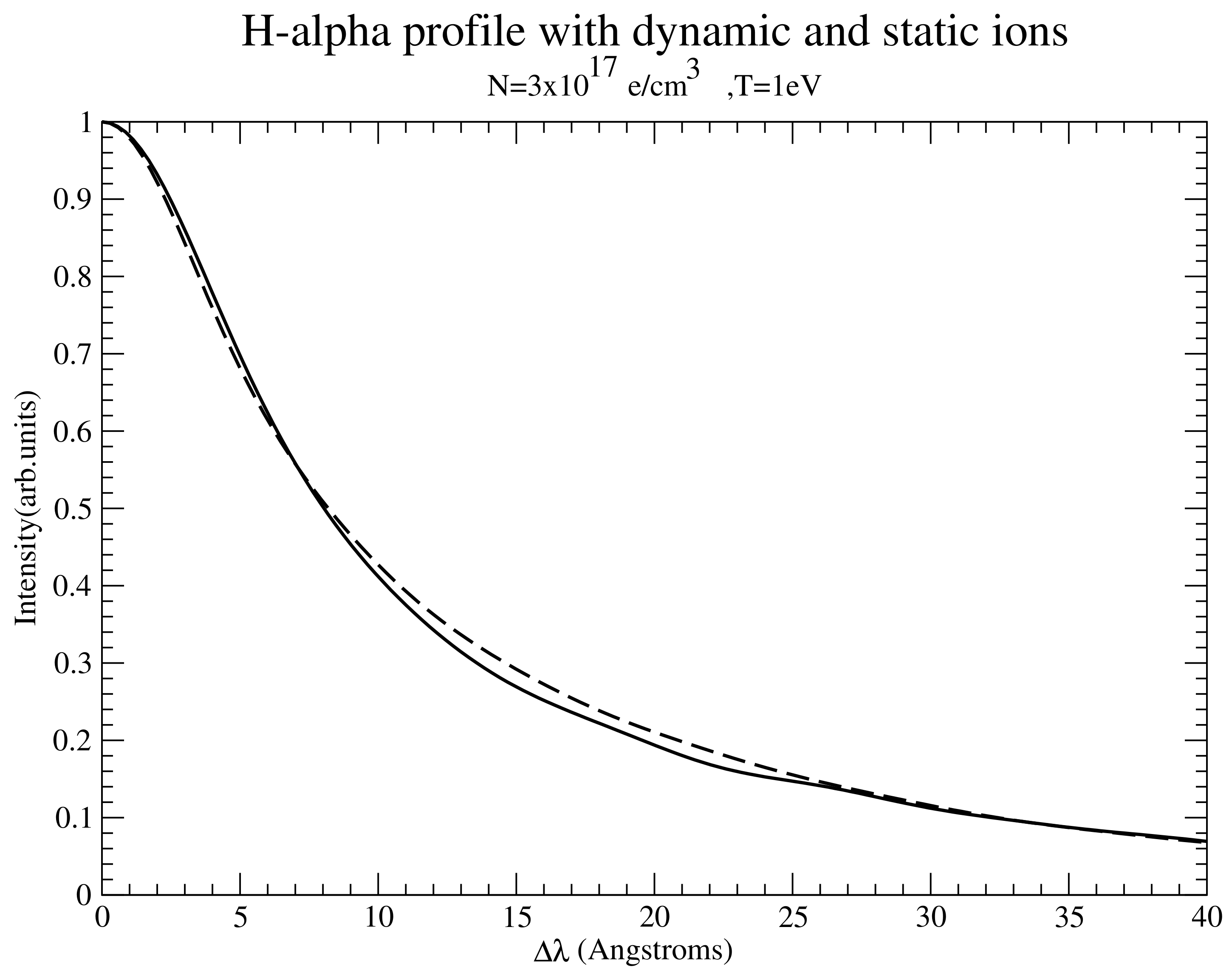
Figure 2.
profile with dynamic (solid) and static (dashed) ions (protons) for a temperature T = 1 eV and electron density e/cm3. The dynamic profile is computed by a joint electron-ion simulation, while the static ion profile is computed by convolution of the dynamic (simulation) electron profile with the quastistatic ion profile.
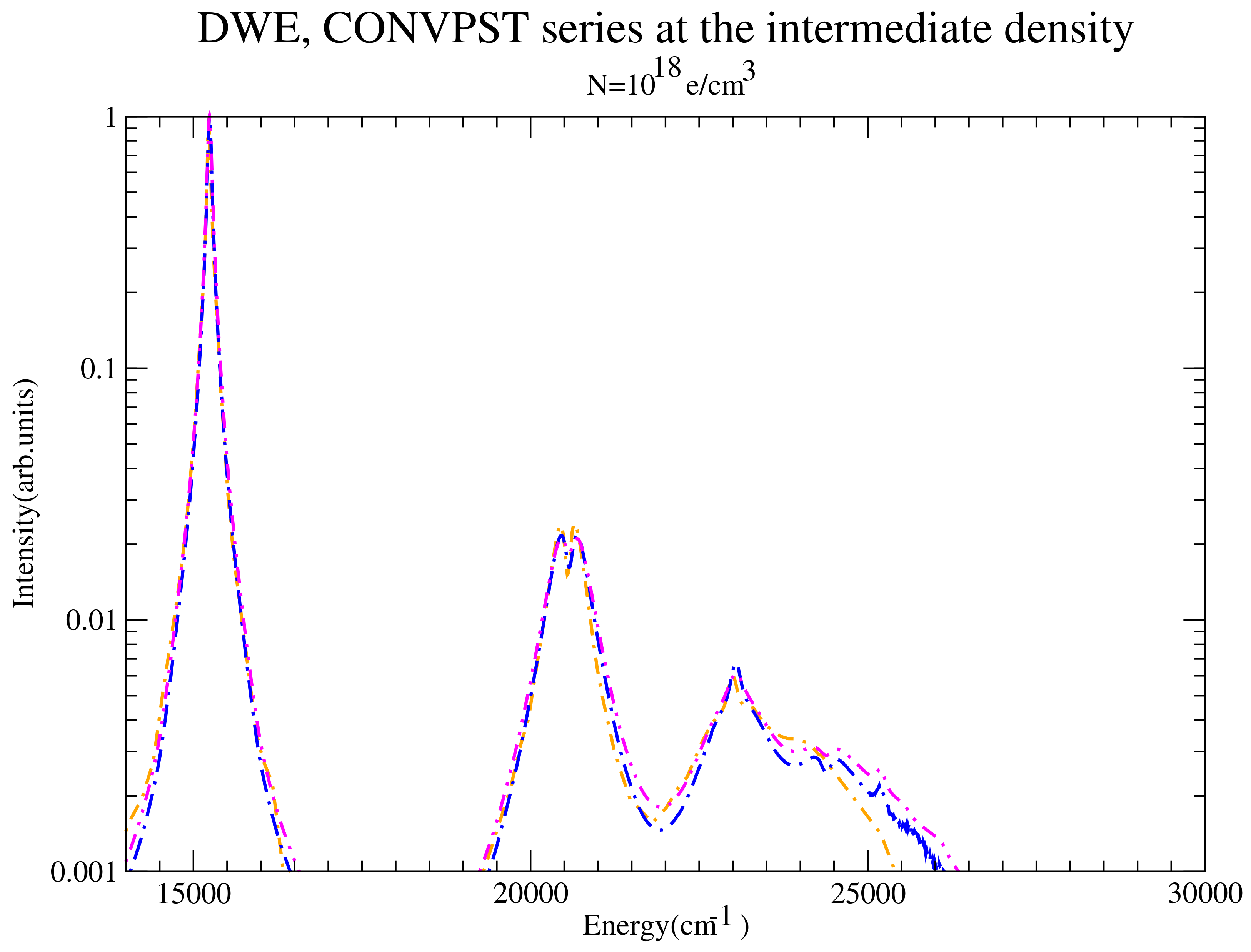
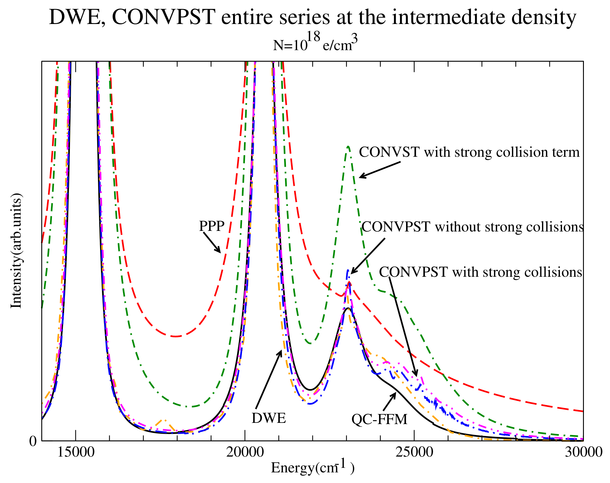
Figure 3.
The entire series for the intermediate density considered for DWE (dash-dotted orange) and CONVPST without (long dash-dotted blue) and with strong collisions (dash-double dotted magenta).
Figure 3.
The entire series for the intermediate density considered for DWE (dash-dotted orange) and CONVPST without (long dash-dotted blue) and with strong collisions (dash-double dotted magenta).
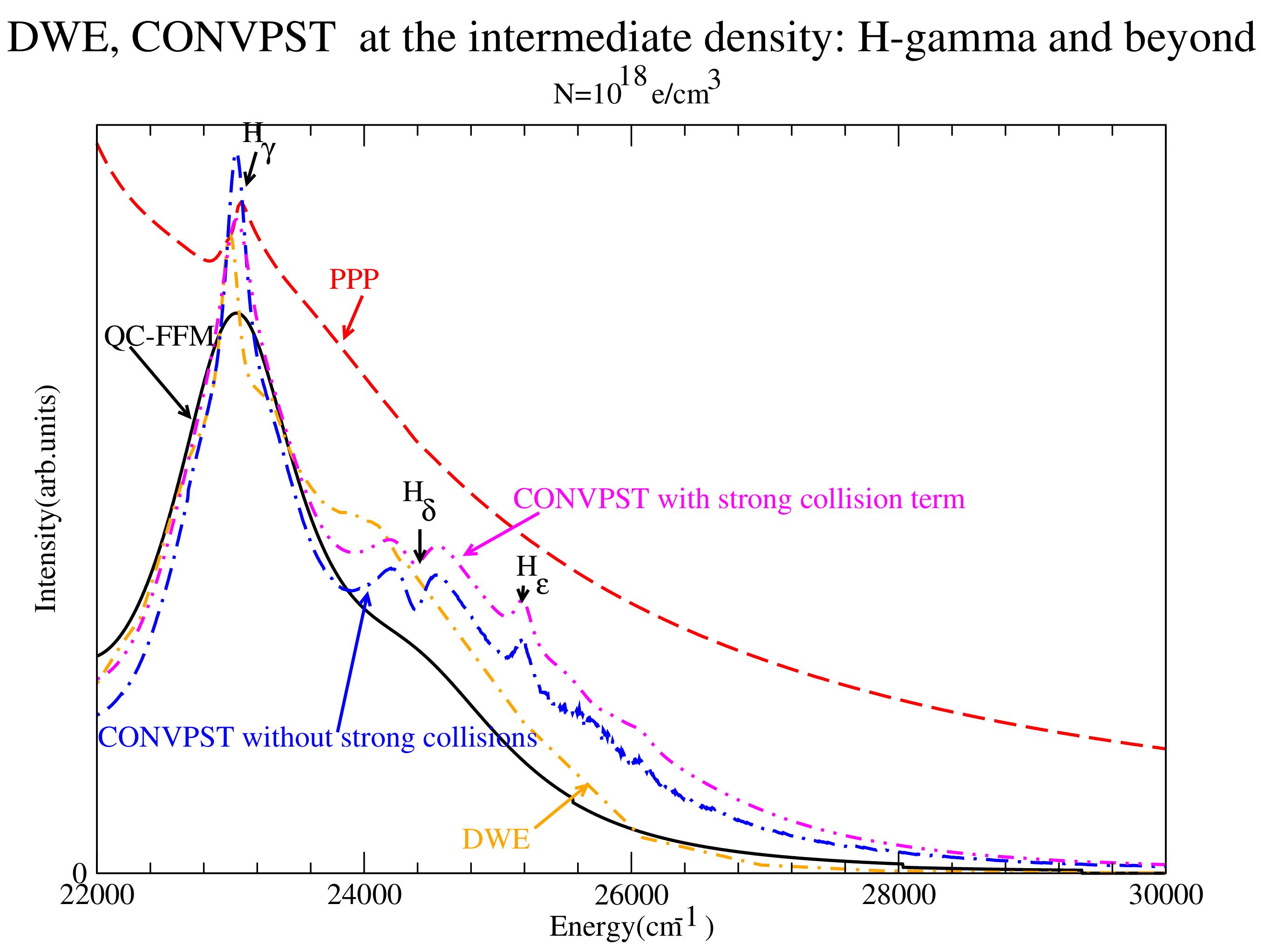
Figure 4.
The series from to the continuum for the intermediate density considered for DWE (dash-dotted orange) and CONVPST without (long dash-dotted blue) and with strong collisions (dash-double dotted magenta). For comparison PPP (red dashed) and QC-FFM (solid black) are also shown.
Figure 4.
The series from to the continuum for the intermediate density considered for DWE (dash-dotted orange) and CONVPST without (long dash-dotted blue) and with strong collisions (dash-double dotted magenta). For comparison PPP (red dashed) and QC-FFM (solid black) are also shown.
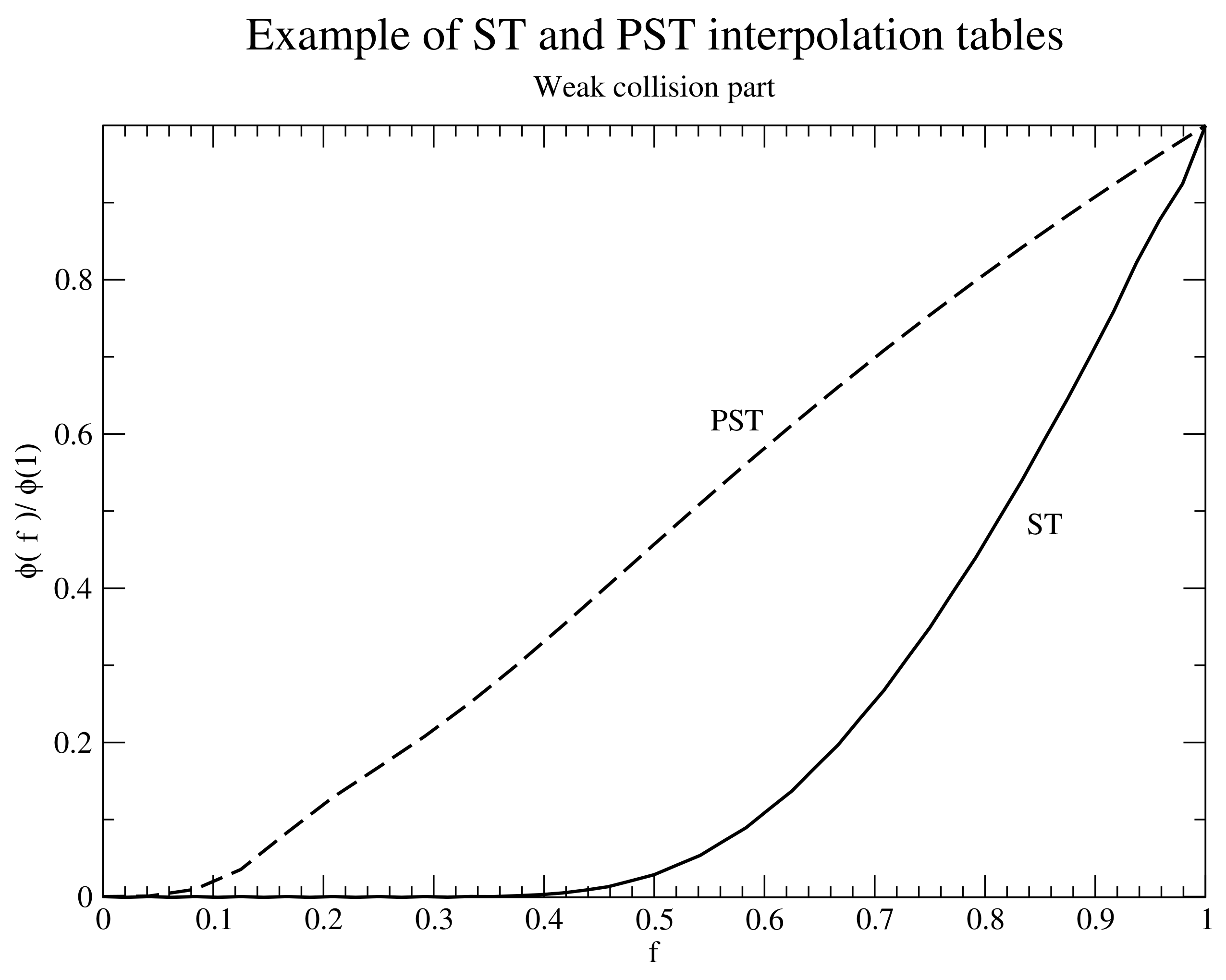
Figure 5.
Illustration of Lewis cutoff interpolation table for both ST (solid) and a single PST “channel” (dashed).
Figure 5.
Illustration of Lewis cutoff interpolation table for both ST (solid) and a single PST “channel” (dashed).
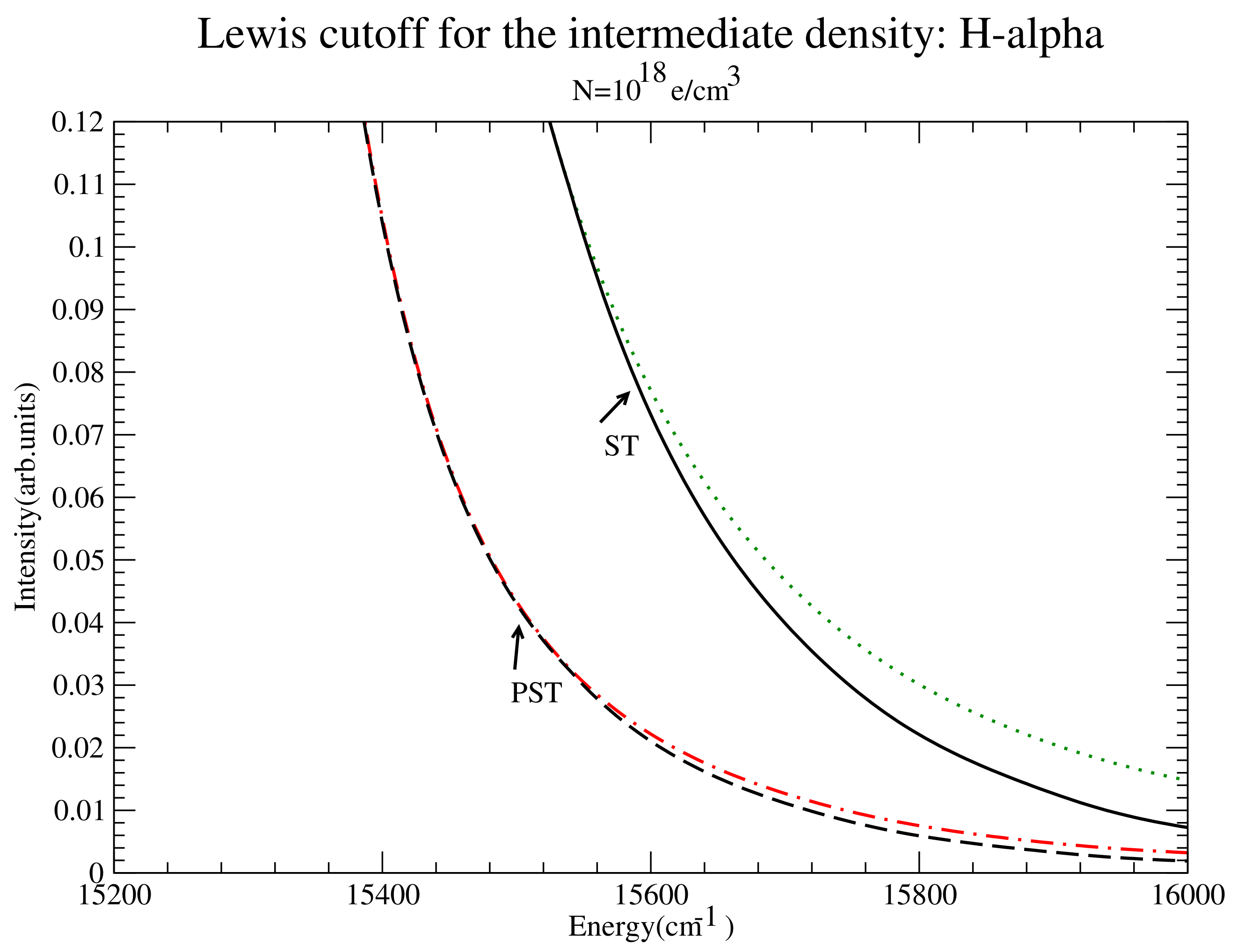
Figure 6.
for CONVST and CONVPST with and without the Lewis cutoff for the intermediate density. Shown are CONVST with Lewis cutoff (black solid), CONVST without Lewis cutoff (green dotted), CONVPST with Lewis cutoff (black dashed) and CONVPST without Lewis cutoff (red dash-dotted).
Figure 6.
for CONVST and CONVPST with and without the Lewis cutoff for the intermediate density. Shown are CONVST with Lewis cutoff (black solid), CONVST without Lewis cutoff (green dotted), CONVPST with Lewis cutoff (black dashed) and CONVPST without Lewis cutoff (red dash-dotted).
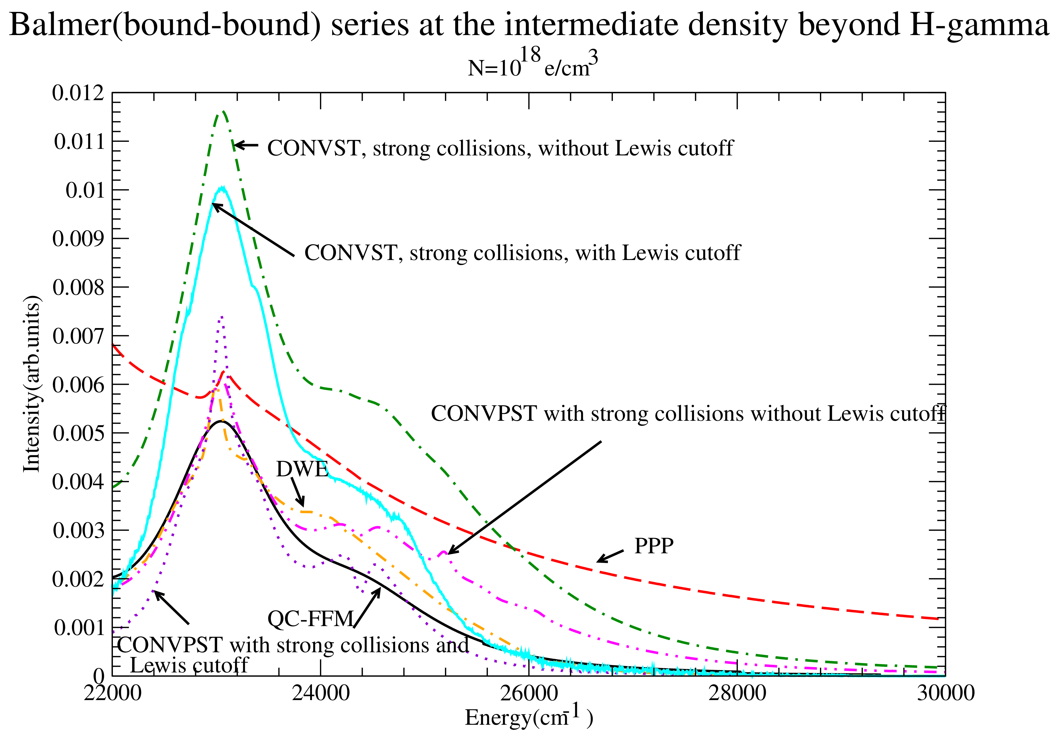
Figure 7.
Balmer Series limit region with and without the Lewis cutoff for the intermediate density. Shown are PPP (red dashed), QC-FFM (back solid) , DWE (orange dash-dotted), CONVST without Lewis cutoff (green dot-double dashed), CONVST with Lewis cutoff (cyan solid), CONVPST without Lewis cutoff (magenta dash-double dotted) and CONVPST with Lewis cutoff (violet dotted). All CONV runs include strong collisions.
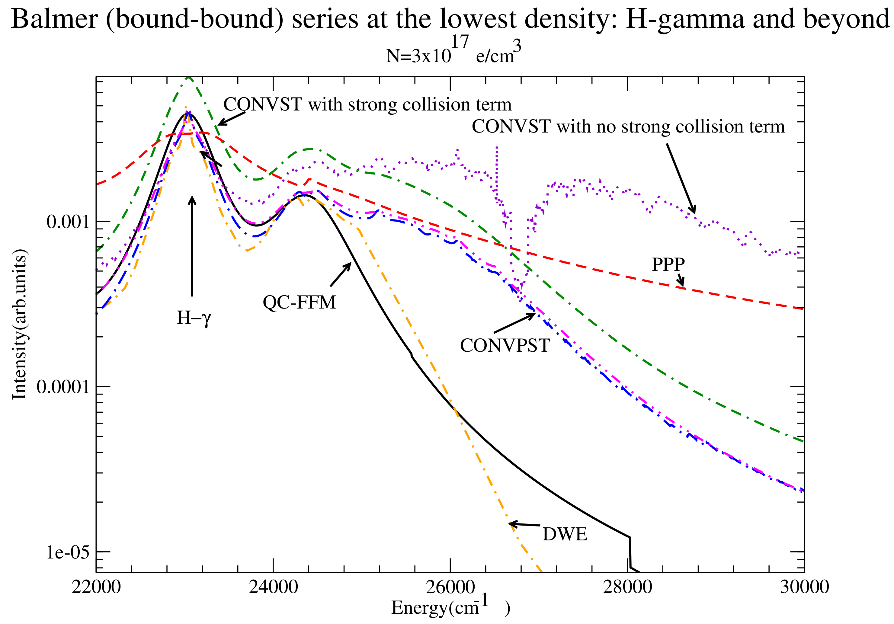
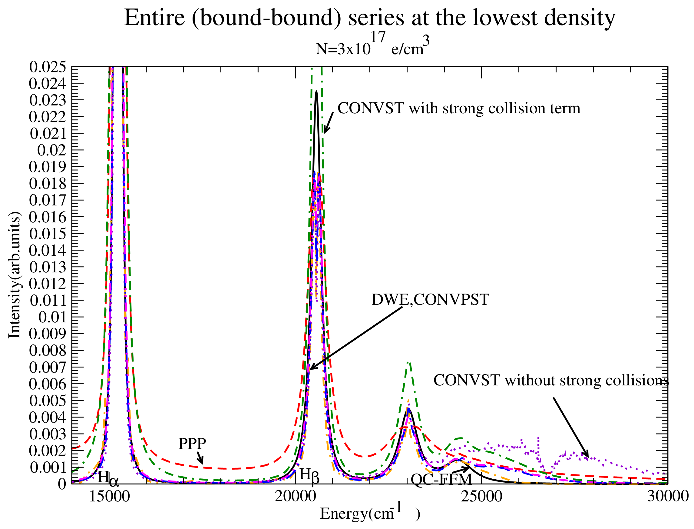
Figure 8.
The entire series for the lowest density considered for QC-FFM (solid black), PPP (dashed red), DWE (dash-dotted orange), CONVST without strong collisions (dotted violet), CONVST with strong collisions (dot-double dashed green), CONVPST without strong collisions (long dash-dotted blue) and CONVPST with strong collisions (dash-double dotted magenta).
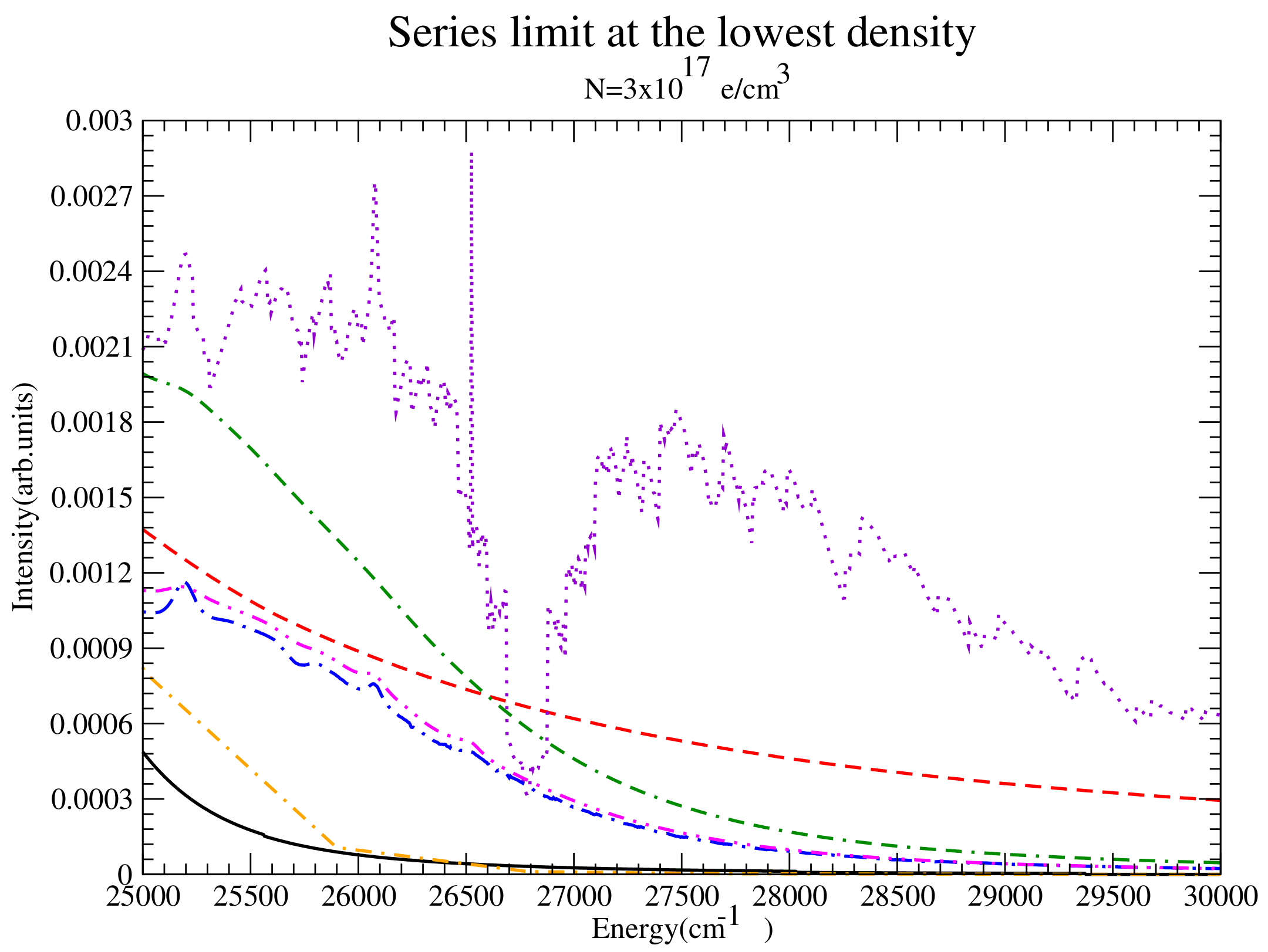
Figure 9.
The series from to the continuum at the lowest density showing fairly small overlap. Shown are QC-FFM (solid), PPP (dashed), DWE (dash-dotted), CONVST without strong collisions (dotted), CONVST with strong collisions (dot-double dashed), CONVPST without strong collisions (long dash-dotted) and CONVPST with strong collisions (dash-double dotted).
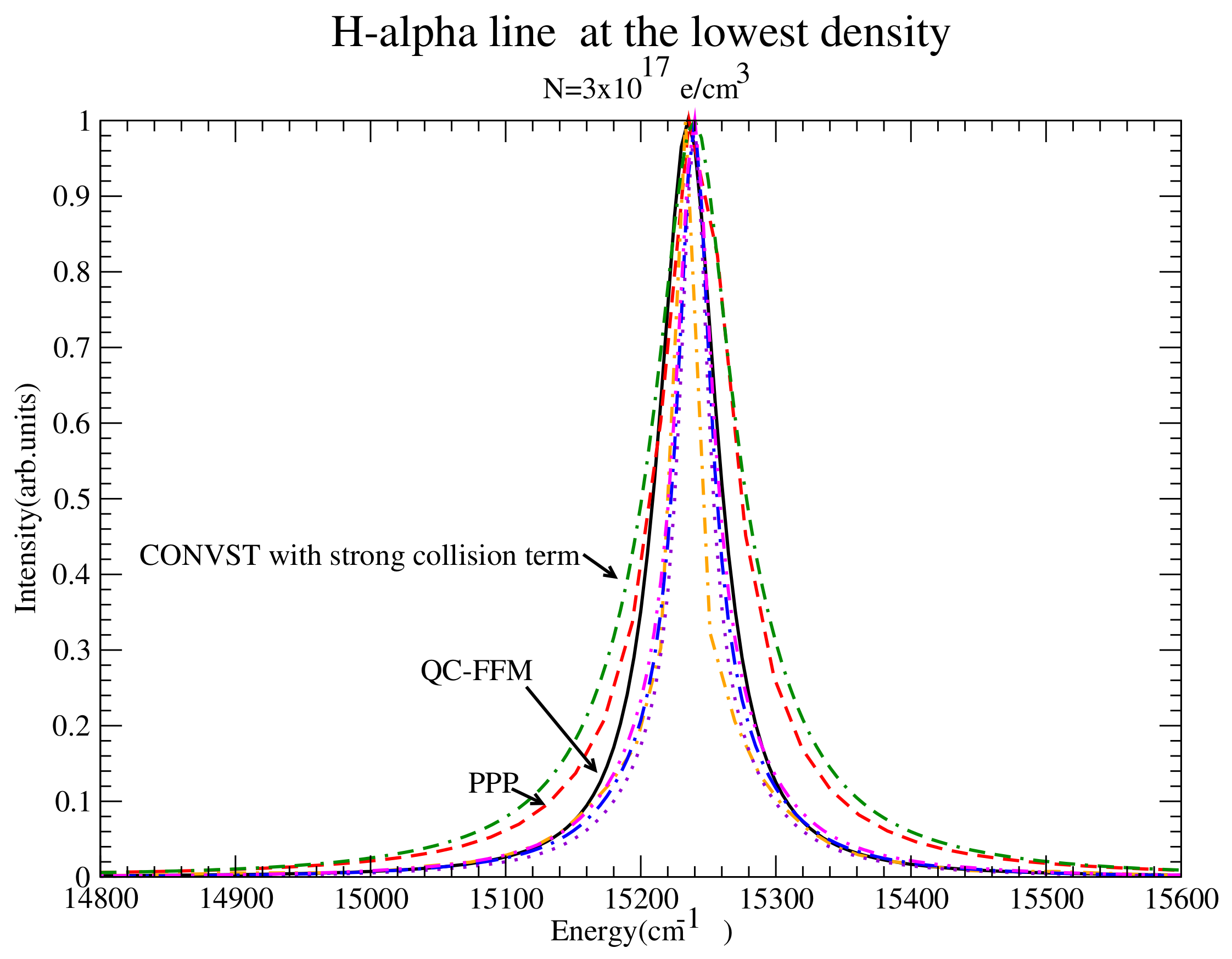
Figure 10.
at the lowest density. Shown are QC-FFM (solid), PPP (dashed), DWE (dash-dotted), CONVST without strong collisions (dotted), CONVST with strong collisions (dot-double dashed), CONVPST without strong collisions (long dash-dotted) and CONVPST with strong collisions (dash-double dotted). Note the good agreement betwen DWE, CONVPST and QC-FFM, while according to most codes, the strong collision term in CONVST appears to significantly overestimate the width, while ignoring it significantly underestimates it. PPP also appears to overestimate the width, as expected due to the GBK operator without frequency dependence.
Figure 11.
Comparision of line widths. Shown are QC-FFM (solid), PPP (dashed), DWE (dash-dotted), CONVST without strong collisions (dotted), CONVST with strong collisions (dot-double dashed), CONVPST without strong collisions (long dash-dotted) and CONVPST with strong collisions (dash-double dotted). It is clear that PPP is widest, probably due to the GBK operator; among the remaining codes it is also clear that the strong collision term adopted by CONVST is too large.
Figure 12.
Comparision of line widths. Shown are QC-FFM (solid), PPP (dashed), DWE (dash-dotted), CONVST without strong collisions (dotted), CONVST with strong collisions (dot-double dashed), CONVPST without strong collisions (long dash-dotted) and CONVPST with strong collisions (dash-double dotted).
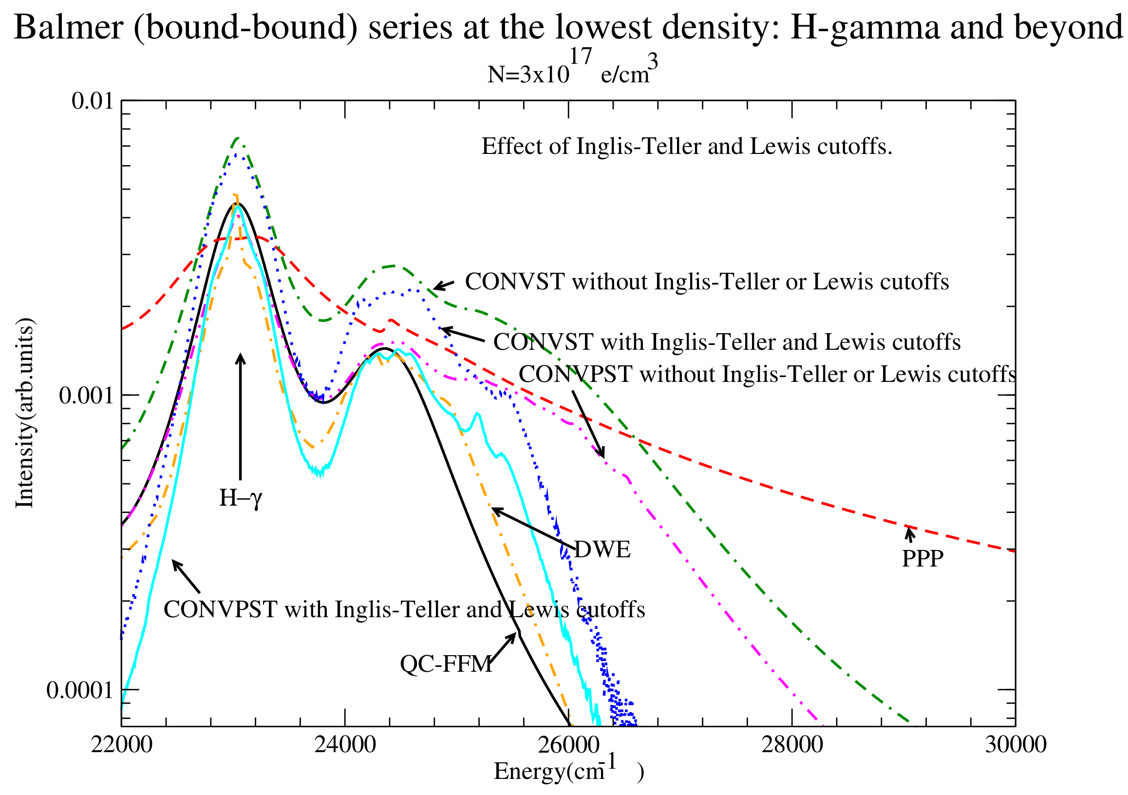
Figure 13.
The series from to the continuum at the lowest density. Shown are QC-FFM (solid black), PPP (dashed red), DWE (dash-dotted), CONVST without the Inglis-Teller or Lewis cutoffs (dot-double dashed green), CONVST with the Inglis-Teller and Lewis cutoffs (dotted blue) CONVPST with the Inglis-Teller and Lewis cutoffs (solid cyan) and CONVPST without the Inglis-Teller or Lewis cutoffs (magenta dash-double dotted). Strong collisions are included in all CONV runs.
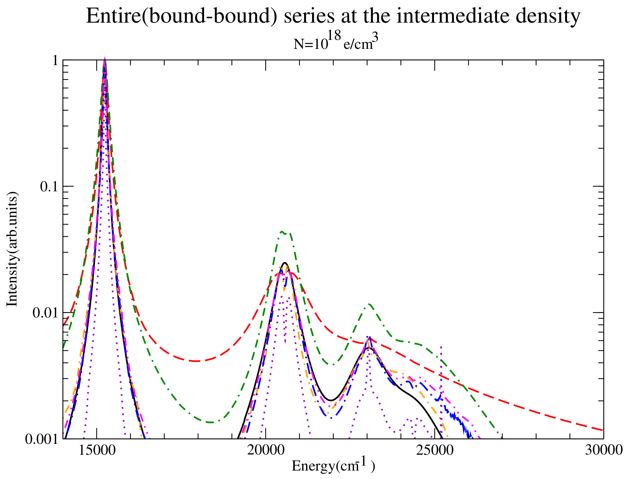
Figure 14.
The entire series for the intermediate density considered for QC-FFM (solid black), PPP (dashed red), DWE (dash-dotted orange), CONVST without strong collisions (dotted violet), CONVST with strong collisions (dot-double dashed green), CONVPST without strong collisions (long dash-dotted blue) and CONVPST with strong collisions (dash-double dotted magenta).
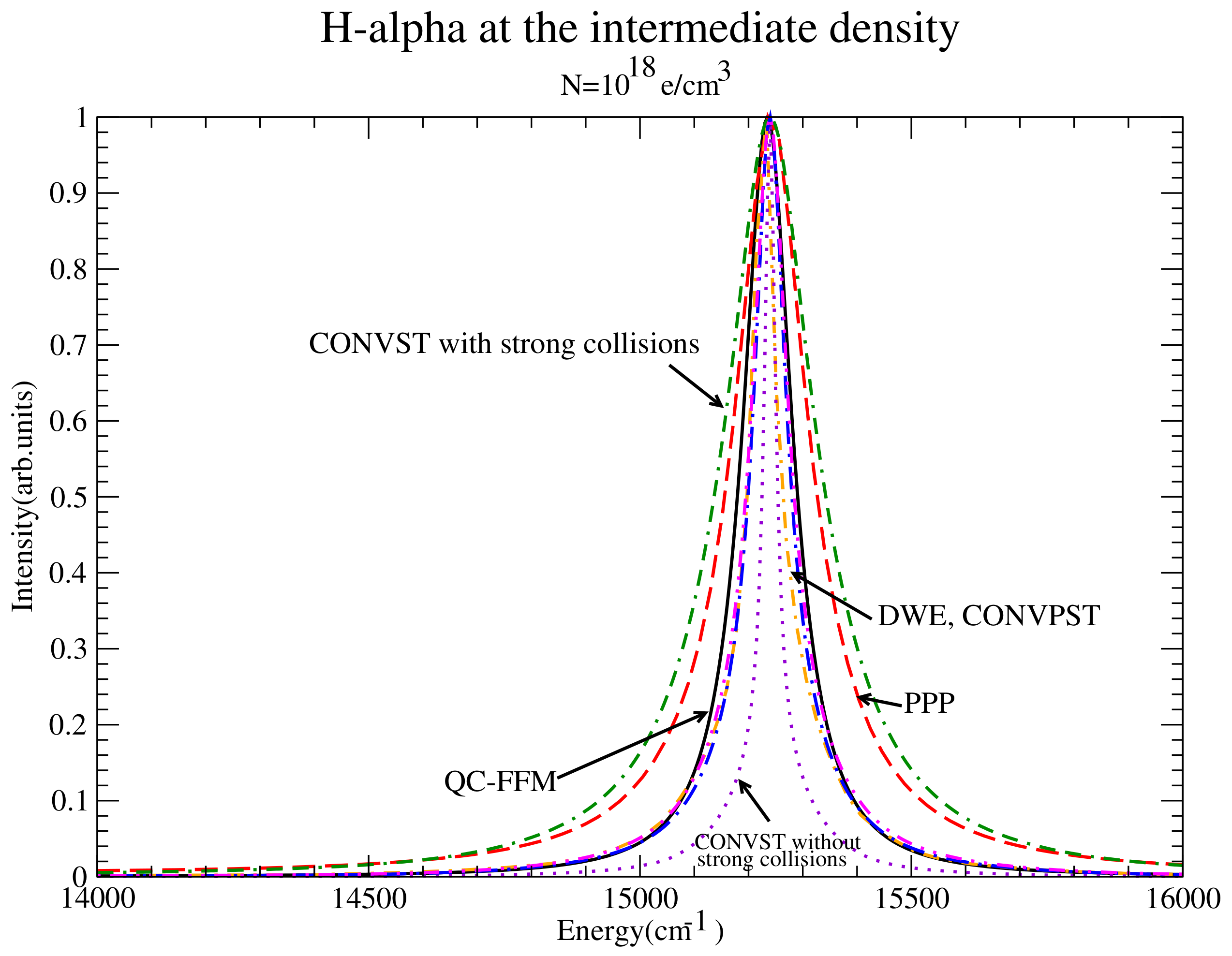
Figure 15.
at the intermediate density showing a very good agreement between QC-FFM, CONVPST and DWE. Shown are QC-FFM (solid), PPP (dashed), DWE (dash-dotted), CONVST without strong collisions (dotted), CONVST with strong collisions (dot-double dashed), CONVPST without strong collisions (long dash-dotted) and CONVPST with strong collisions (dash-double dotted).
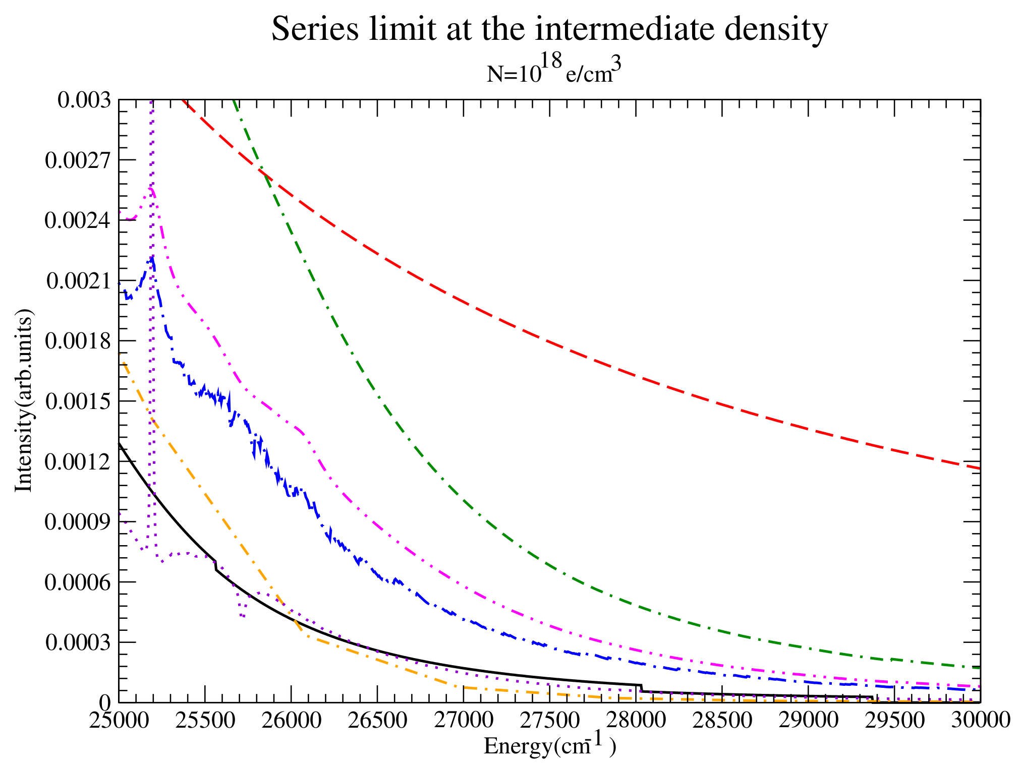
Figure 16.
The series from to the continuum for the intermediate density considered for DWE (dash-dotted orange) and CONVPST without (long dash-dotted blue) and with strong collisions (dash-double dotted magenta). For comparison PPP (red dashed) and QC-FFM (solid black) are also shown.
Figure 16.
The series from to the continuum for the intermediate density considered for DWE (dash-dotted orange) and CONVPST without (long dash-dotted blue) and with strong collisions (dash-double dotted magenta). For comparison PPP (red dashed) and QC-FFM (solid black) are also shown.
Figure 17.
Comparision of line widths. Shown are QC-FFM (solid), PPP (dashed), DWE (dash-dotted), CONVST without strong collisions (dotted), CONVST with strong collisions (dot-double dashed), CONVPST without strong collisions (long dash-dotted) and CONVPST with strong collisions (dash-double dotted).
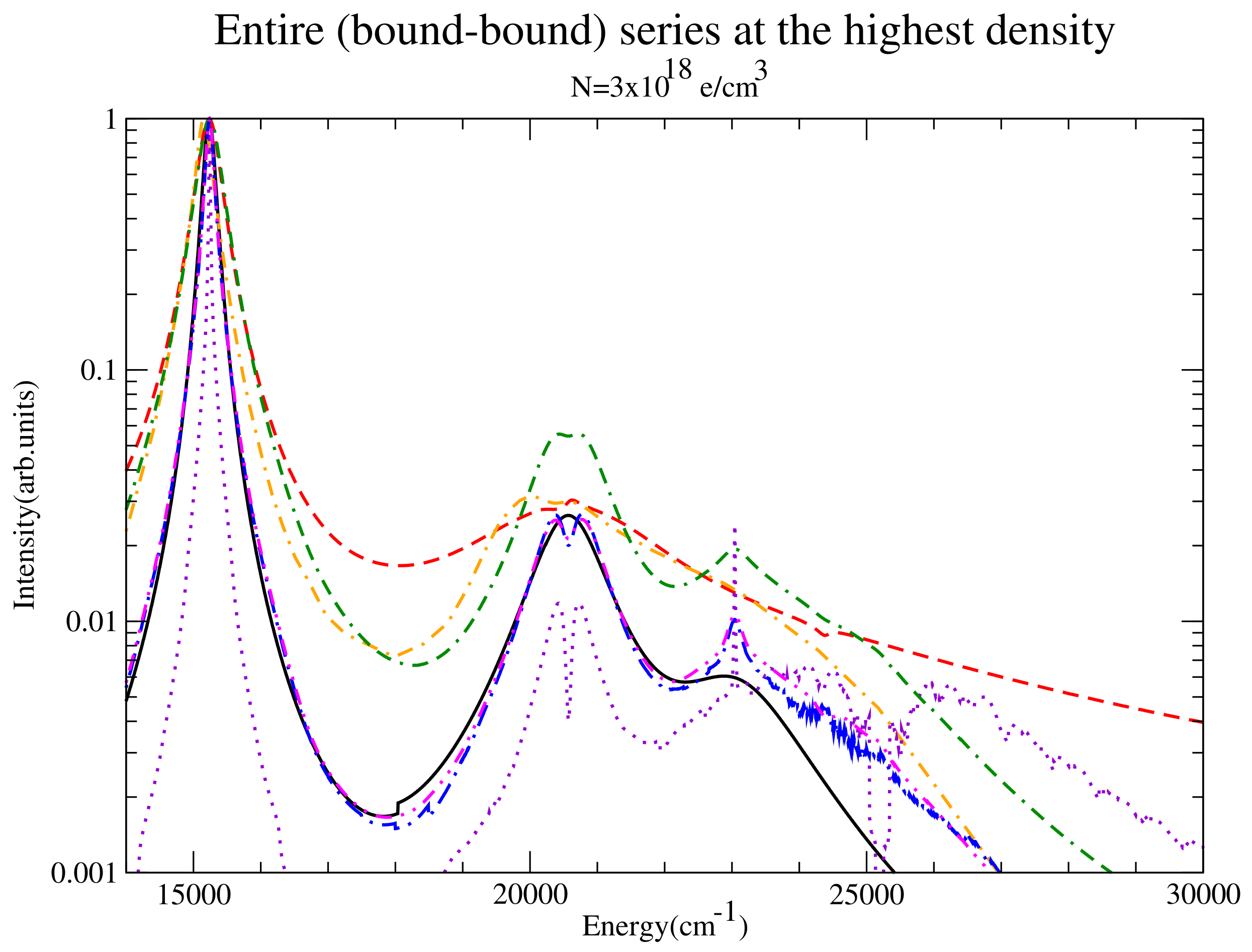
Figure 18.
The entire series at the highest density. Shown are QC-FFM (solid), PPP (dashed), DWE (dash-dotted), CONVST without strong collisions (dotted), CONVST with strong collisions (dot-double dashed), CONVPST without strong collisions (long dash-dotted) and CONVPST with strong collisions (dash-double dotted).
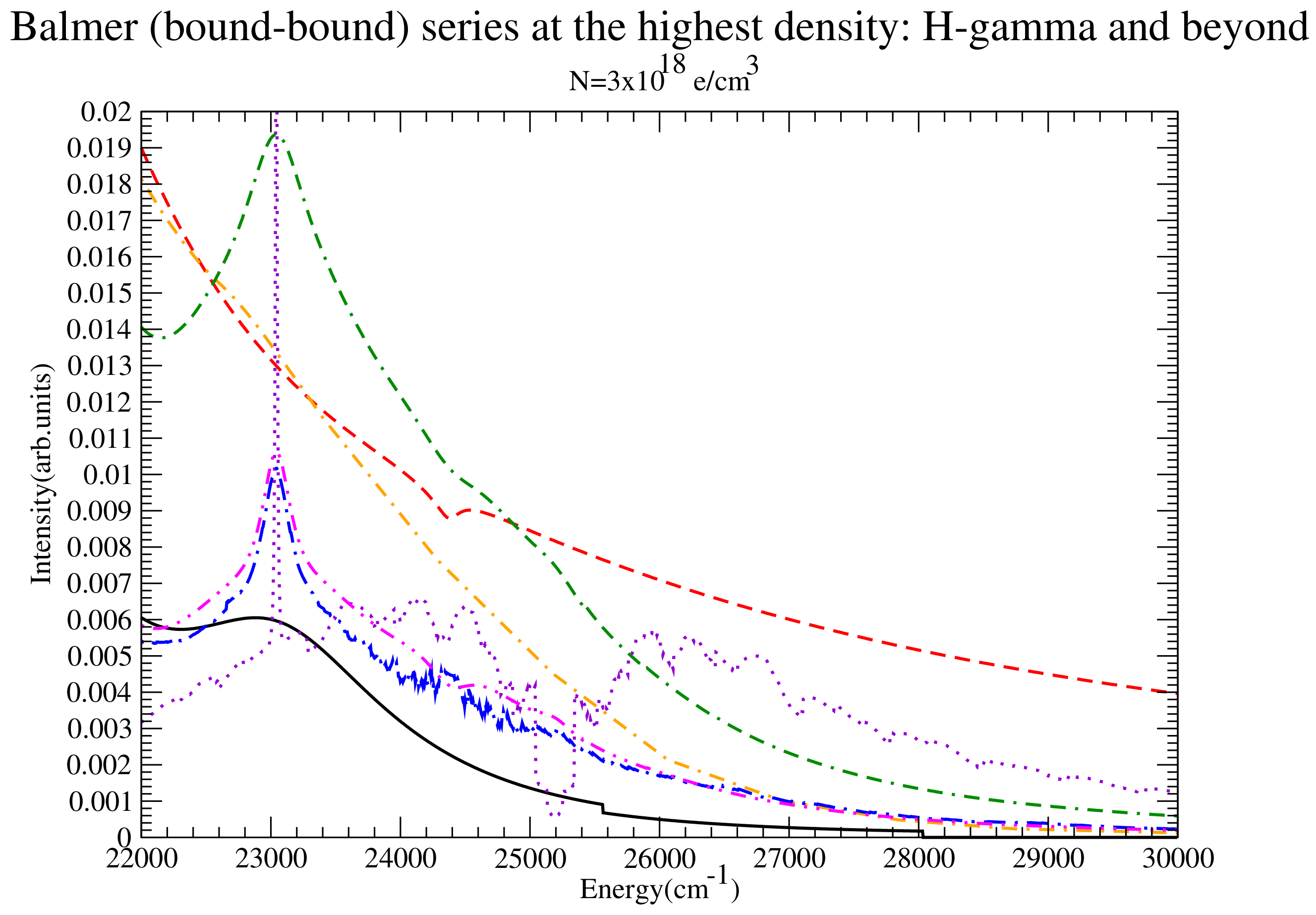
Figure 19.
The region including and beyond at the highest density. Shown are QC-FFM (solid), PPP (dashed), DWE (dash-dotted), CONVST without strong collisions (dotted), CONVST with strong collisions (dot-double dashed), CONVPST without strong collisions (long dash-dotted) and CONVPST with strong collisions (dash-double dotted).
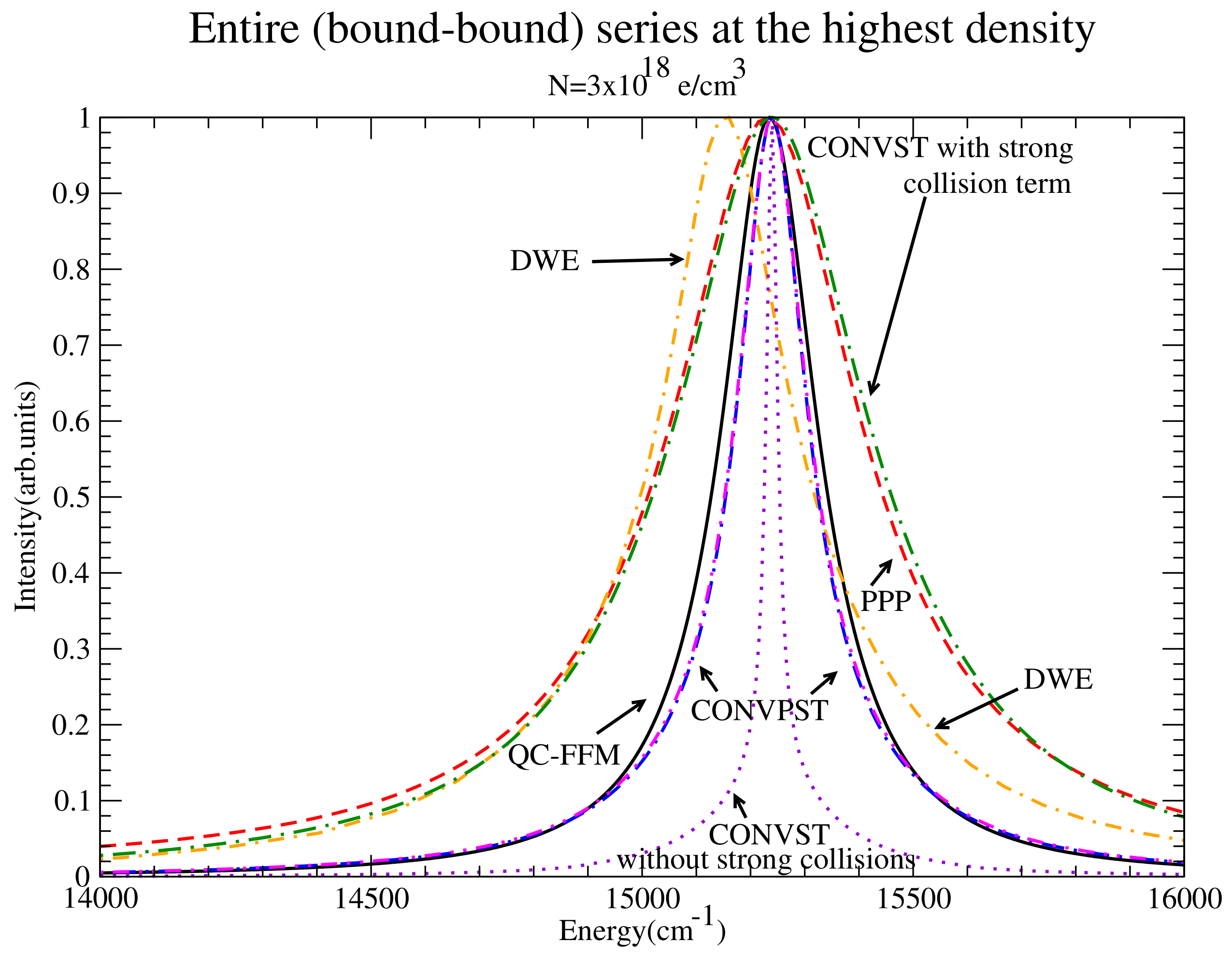
Figure 20.
at the highest density showing a very good agreement between QC-FFM and CONVPST. Shown are QC-FFM (solid), PPP (dashed), DWE (dash-dotted), CONVST without strong collisions (dotted), CONVST with strong collisions (dot-double dashed), CONVPST without strong collisions (long dash-dotted) and CONVPST with strong collisions (dash-double dotted).
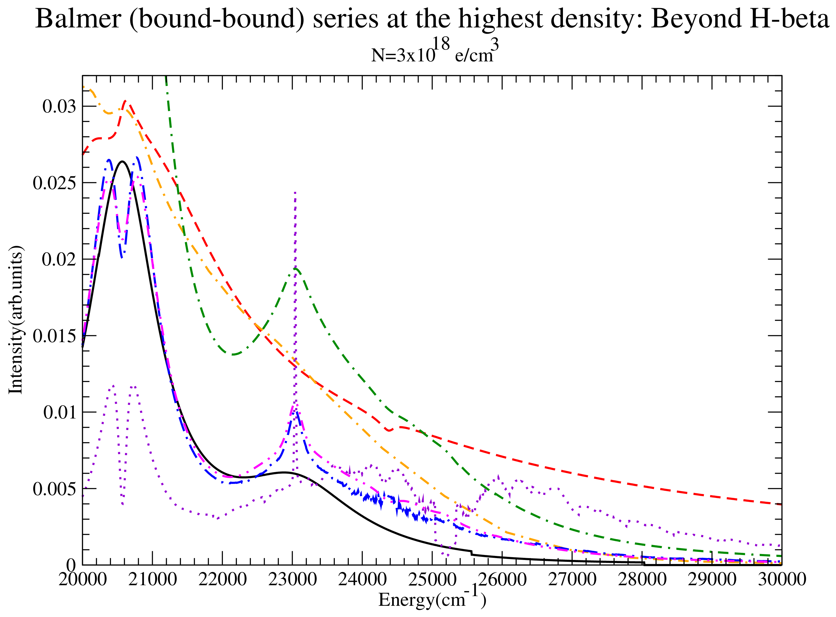
Figure 21.
The region including and beyond at the highest density showing a very good agreement between QC-FFM and CONVPST up until . Shown are QC-FFM (solid), PPP (dashed), DWE (dash-dotted), CONVST without strong collisions (dotted), CONVST with strong collisions (dot-double dashed), CONVPST without strong collisions (long dash-dotted) and CONVPST with strong collisions (dash-double dotted).
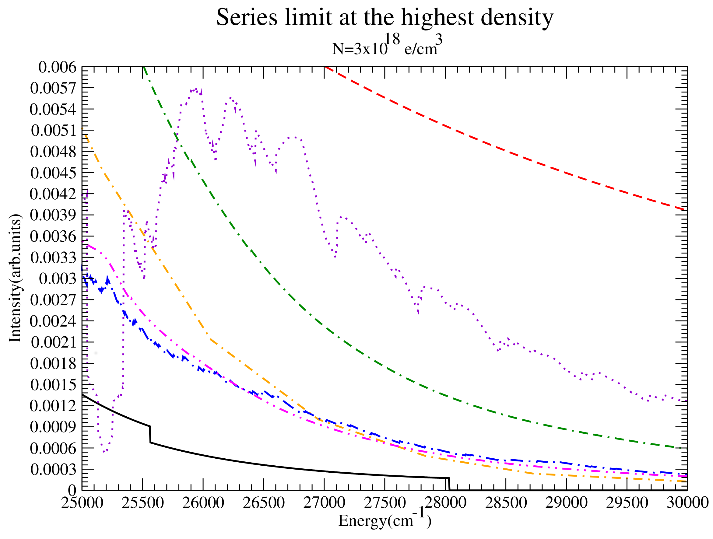
Figure 22.
The region near the series limit at the highest density. Shown are QC-FFM (solid), PPP (dashed), DWE (dash-dotted), CONVST without strong collisions (dotted), CONVST with strong collisions (dot-double dashed), CONVPST without strong collisions (long dash-dotted) and CONVPST with strong collisions (dash-double dotted).
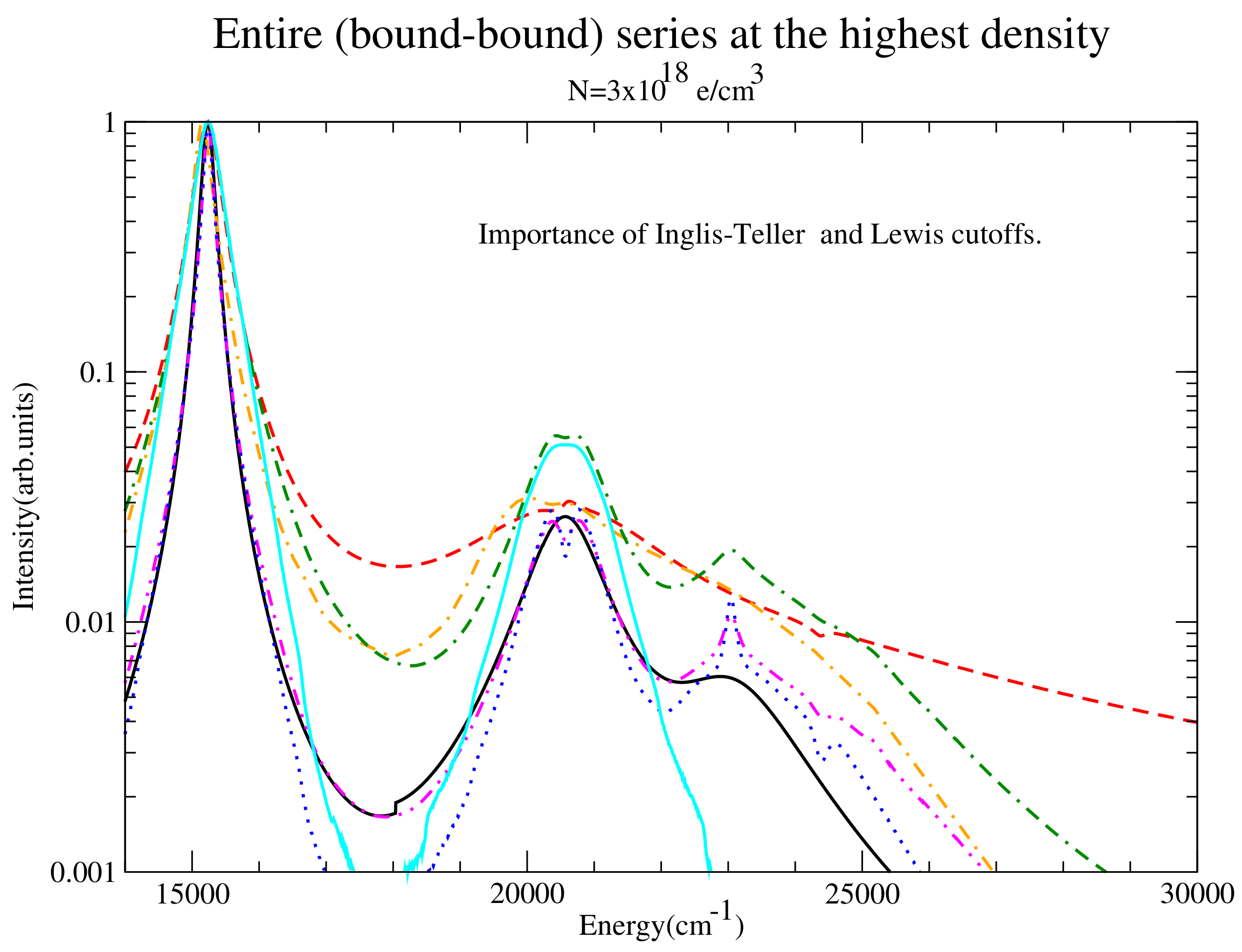
Figure 23.
The entire series at the highest density. Shown are QC-FFM (black solid), PPP (red dashed), DWE (orange dash-dotted), CONVST without Inglis-Teller or Lewis cutoff (green dot-double dashed), CONVST with Inglis-Teller and Lewis cutoff (cyan solid), CONVPST without Inglis-Teller or Lewis cutoff (magenta dash-double dotted) and CONVPST with Inglis-Teller and Lewis cutoff (blue dotted). All CONVST/PST runs include strong collisions.
Figure 24.
BB + FB vs. BB comparison for the line at the intermediate density. Shown CONVST for BB + FB (blue solid) and CONVST for BB + FB (red solid) and the corresponding BB only results (dashed), which are identical.
Figure 24.
BB + FB vs. BB comparison for the line at the intermediate density. Shown CONVST for BB + FB (blue solid) and CONVST for BB + FB (red solid) and the corresponding BB only results (dashed), which are identical.
Figure 25.
BB + FB vs. BB comparison for the lowest density close to the continuum. Shown are QC-FFM for BB + FB (solid) and BB only (dot-double dashed), CONVST for BB + FB (dashed) and CONVST for BB only (dash-dotted) and CONVPST for FB + BB (dotted) and BB only (dash-double dotted).
Figure 25.
BB + FB vs. BB comparison for the lowest density close to the continuum. Shown are QC-FFM for BB + FB (solid) and BB only (dot-double dashed), CONVST for BB + FB (dashed) and CONVST for BB only (dash-dotted) and CONVPST for FB + BB (dotted) and BB only (dash-double dotted).
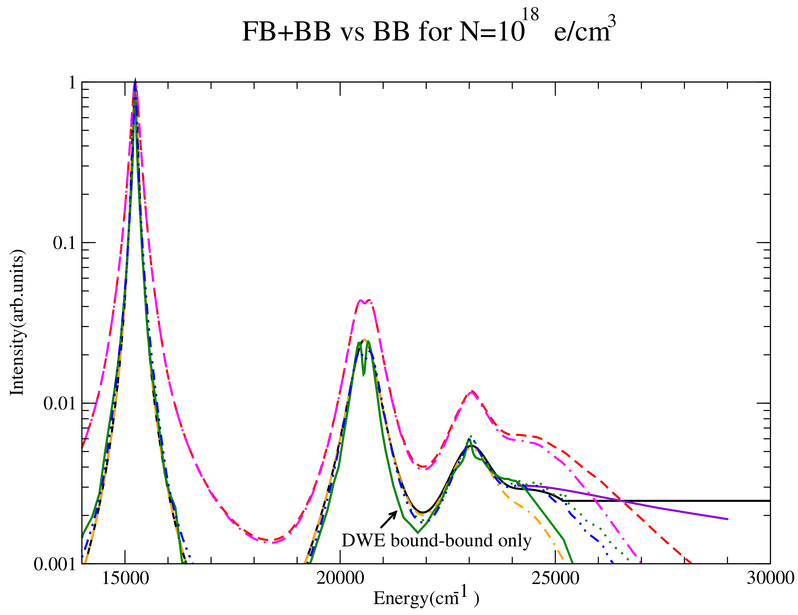
Figure 26.
BB + FB vs. BB comparison for the intermediate density close to the continuum. Shown are QC-FFM for BB + FB (solid) and BB only (dot-double dashed), CONVST for BB + FB (dashed) and CONVST for BB only (dash-dotted) and CONVPST for FB + BB (dotted) and BB only (dash-double dotted). Also shown is DWE (green solid) for the BB spectrum.
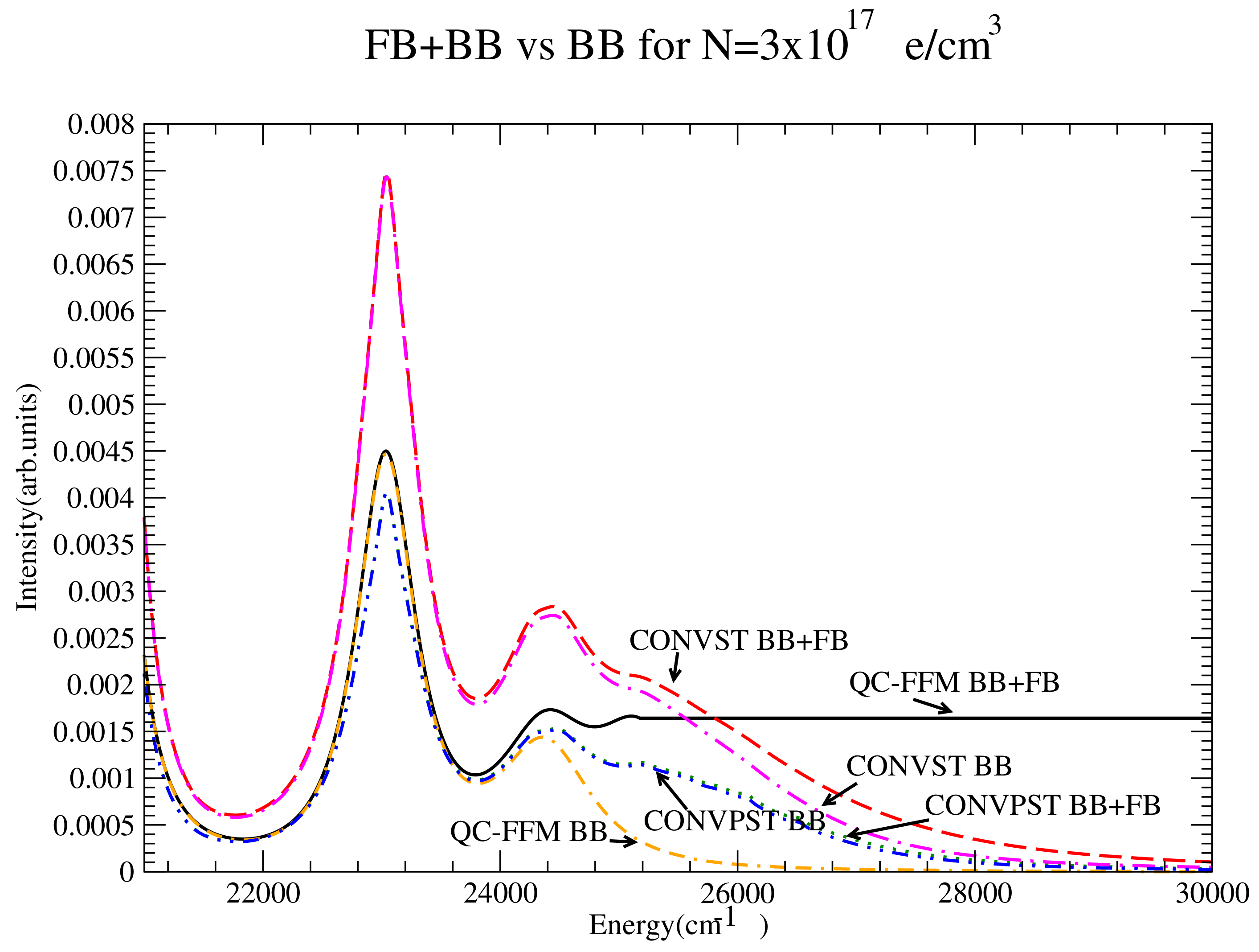
Figure 27.
BB + FB vs. BB comparison for the highest density close to the continuum. Shown are QC-FFM for BB + FB (solid) and BB only (dot-double dashed), CONVST for BB + FB (dashed) and CONST for BB only (dash-dotted) and CONVPST for FB + BB (dotted) and BB only (dash-double dotted).
Figure 27.
BB + FB vs. BB comparison for the highest density close to the continuum. Shown are QC-FFM for BB + FB (solid) and BB only (dot-double dashed), CONVST for BB + FB (dashed) and CONST for BB only (dash-dotted) and CONVPST for FB + BB (dotted) and BB only (dash-double dotted).
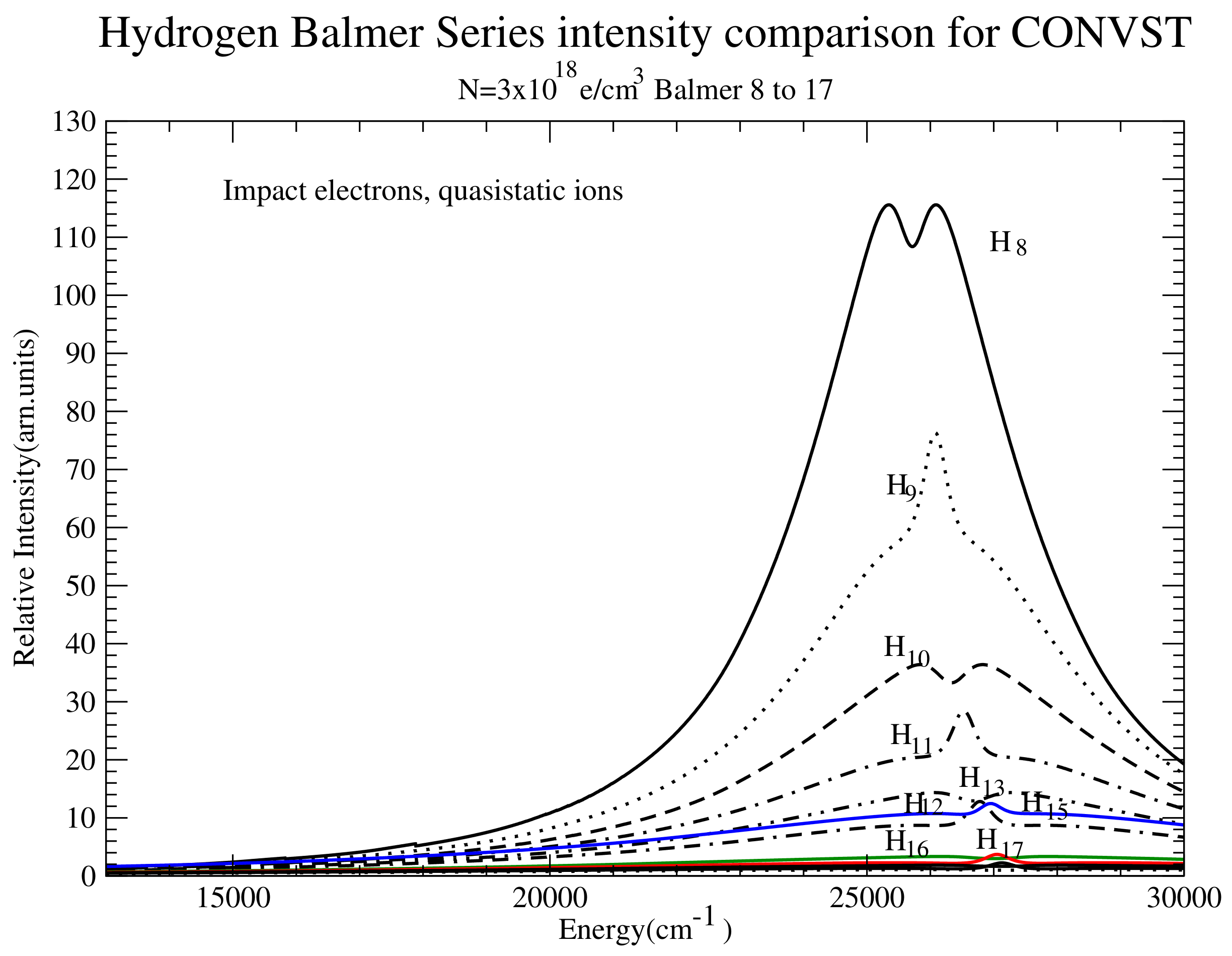
Figure 28.
Intensity comparison for Balmer 8 to Balmer 17 at the highest density. Shown are CONVST profiles for (solid black), (dotted), (dashed), (dash-dotted), (dash-double dotted), (dot double dashed), (solid blue), (solid green) and (solid red).
Figure 28.
Intensity comparison for Balmer 8 to Balmer 17 at the highest density. Shown are CONVST profiles for (solid black), (dotted), (dashed), (dash-dotted), (dash-double dotted), (dot double dashed), (solid blue), (solid green) and (solid red).
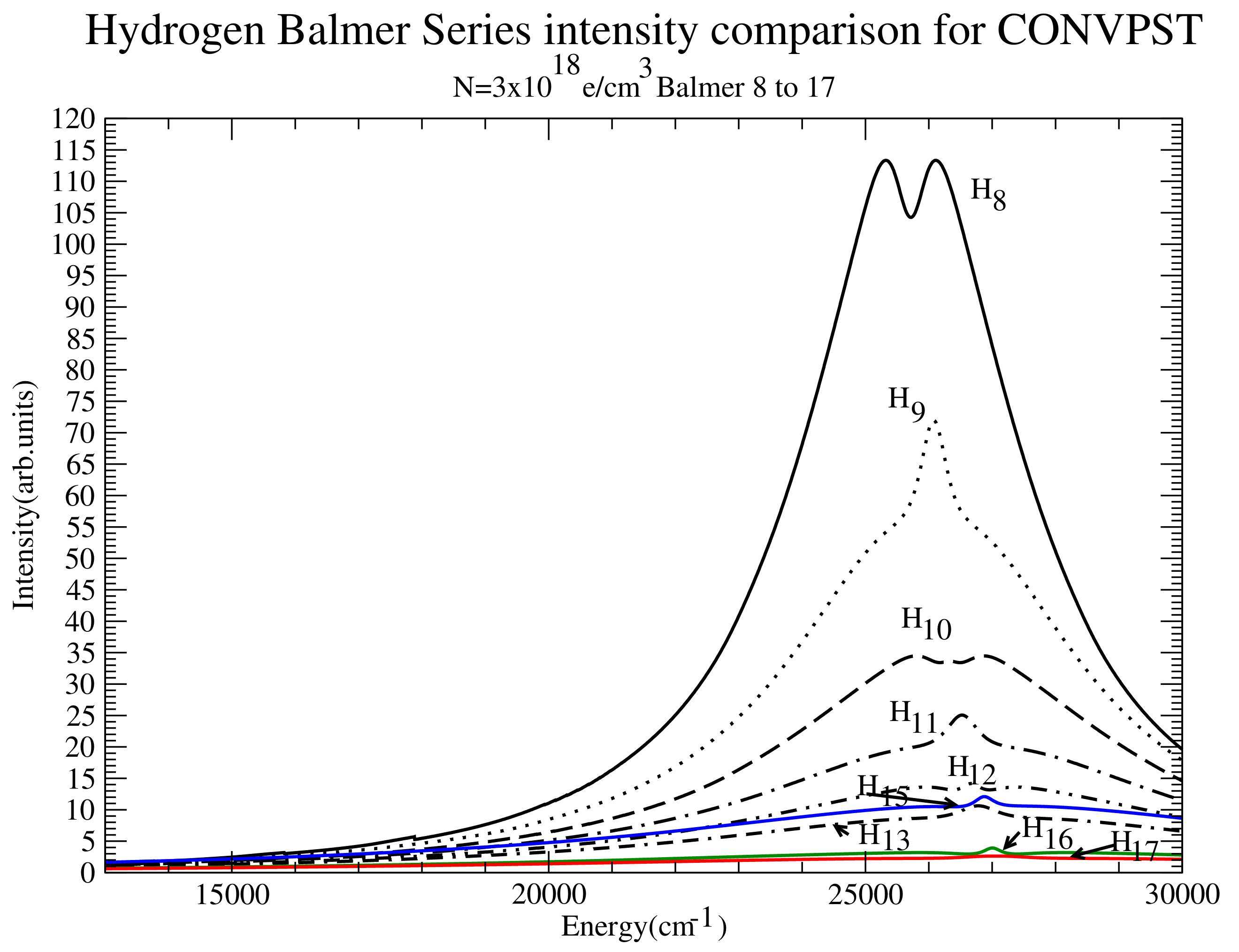
Figure 29.
Intensity comparison for Balmer 8 to Balmer 17 at the highest density. Shown are CONVPST profiles for (solid black), (dotted), (dashed), (dash-dotted), (dash-double dotted), (dot double dashed), (solid blue), (solid green) and (solid red).
Figure 29.
Intensity comparison for Balmer 8 to Balmer 17 at the highest density. Shown are CONVPST profiles for (solid black), (dotted), (dashed), (dash-dotted), (dash-double dotted), (dot double dashed), (solid blue), (solid green) and (solid red).
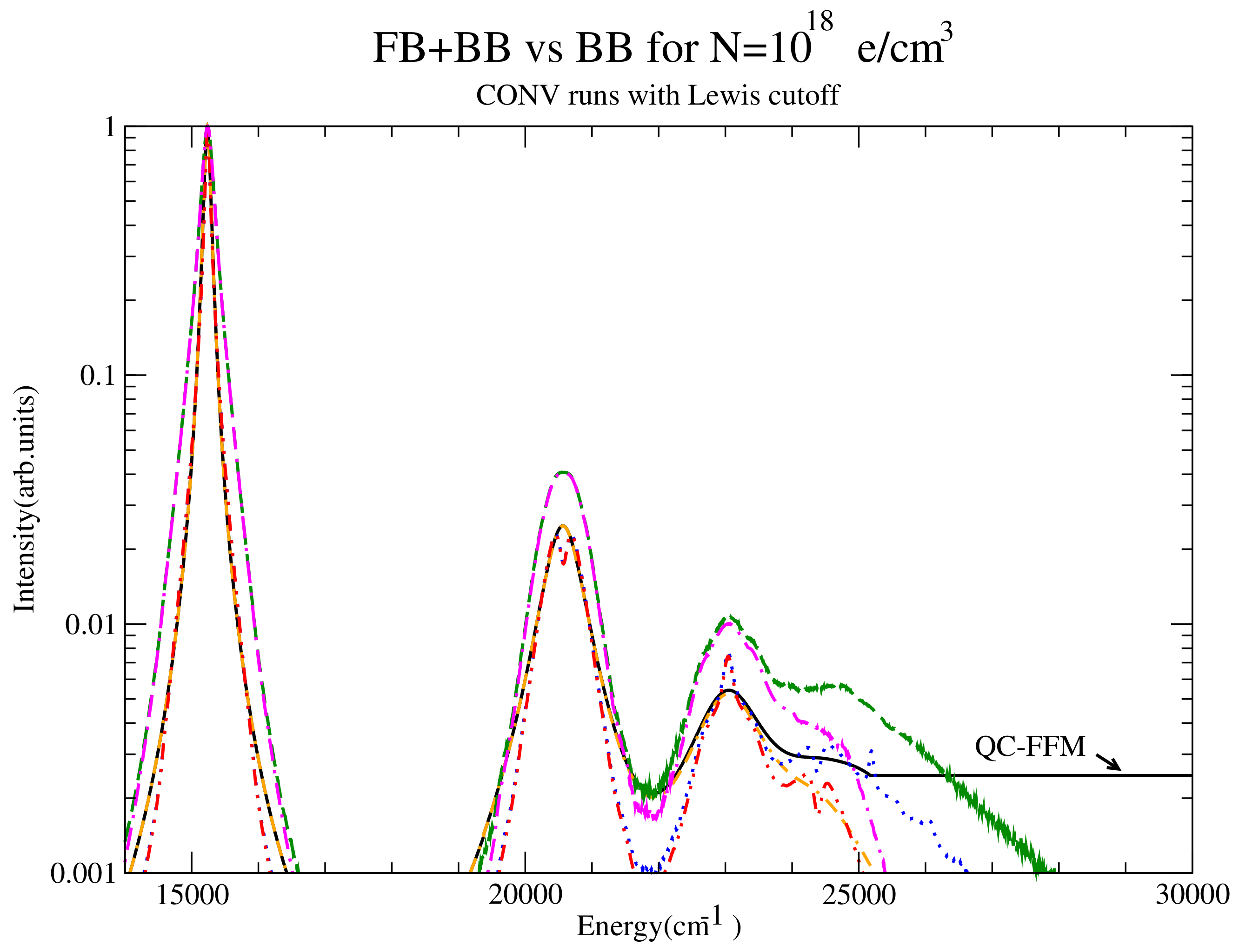
Figure 30.
BB + FB vs. BB comparison for the intermediate density close to the continuum. Shown are QC-FFM for BB + FB (solid black) and BB only (dot-double dashed orange), CONVST for BB + FB (dashed green) and CONVST for BB only (dash-dotted magenta) and CONVPST for FB + BB (dotted blue) and BB only (dash-double dotted red). The CONV runs include strong collisions and the Lewis cutoff. The Inglis-Teller cutoff was used in the BB only CONV results.
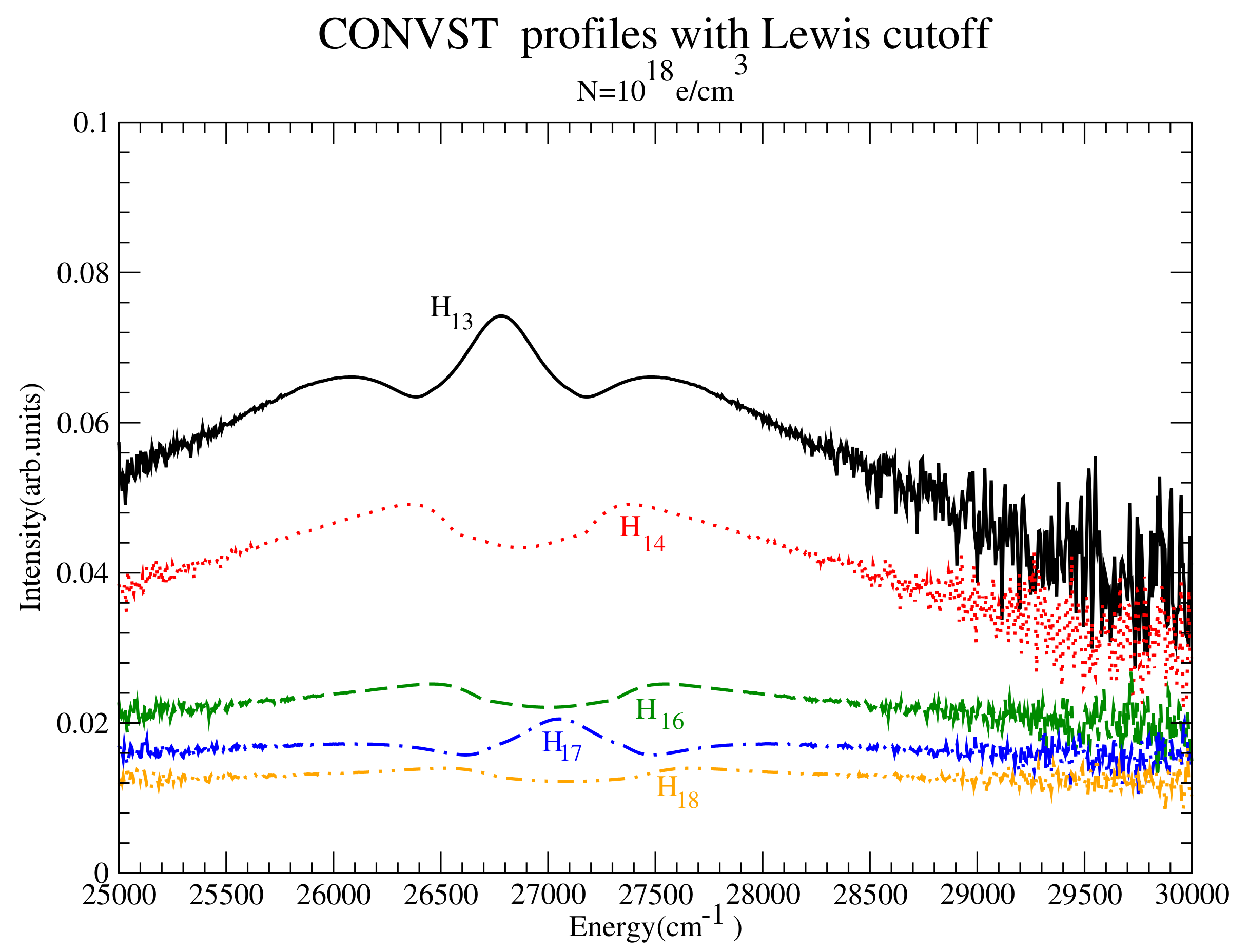
Figure 31.
Intensity comparison for Balmer 13 to Balmer 18 at the intermediate density. Shown are CONVST profiles for (solid black), (dotted red), (dashed green), (dash-dotted blue) and (dash-double dotted orange).
Figure 31.
Intensity comparison for Balmer 13 to Balmer 18 at the intermediate density. Shown are CONVST profiles for (solid black), (dotted red), (dashed green), (dash-dotted blue) and (dash-double dotted orange).
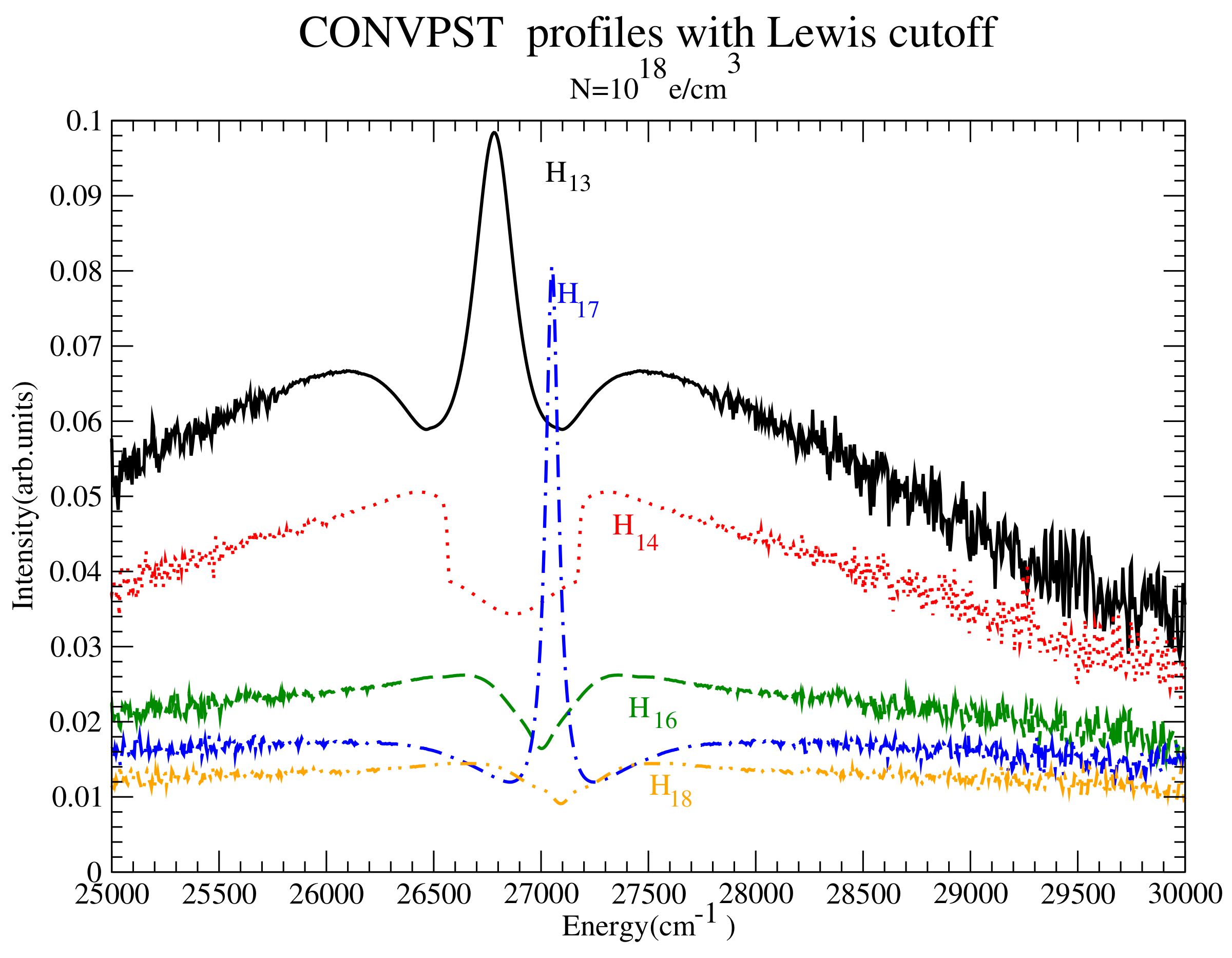
Figure 32.
Intensity comparison for Balmer 13 to Balmer 18 at the intermediate density. Shown are CONVPST profiles for (solid black), (dotted red), (dashed green), (dash-dotted blue) and (dash-double dotted orange).
Figure 32.
Intensity comparison for Balmer 13 to Balmer 18 at the intermediate density. Shown are CONVPST profiles for (solid black), (dotted red), (dashed green), (dash-dotted blue) and (dash-double dotted orange).
Table 1.
Line broadening issues and their importance for line mergings.
Table 1.
Line broadening issues and their importance for line mergings.
| Issue | Importance (Y/N) | Comment |
|---|
| Ion Dynamics | N | For the entire series |
| Strong Collisions | Y | For the high n-lines |
| Penetrating Collisions | Y | For the high n-lines |
| Quantum effects | N | Could be for lower temperatures |
Table 2.
Relative importance of penetration for all lines in the series and plasma parameters considered in the workshop examples. is displayed as a function of the electron density N for all series lines considered in the bound-bound spectrum calculation. The density N is expressed in units of e/cm3. Bold is used for cases where the strong collision term is comparable to or dominates the weak collision contribution.
| N | | | | | | | | | | |
|---|
| 3 | 2.96 | 2.39 | 1.94 | 1.58 | 1.27 | 1 | 0.77 | 0.56 | 0.365 | 0.19 |
| 10 | 2.36 | 1.79 | 1.34 | 0.97 | 0.67 | 0.4 | 0.165 | | |
| 30 | 1.81 | 1.24 | 0.79 | 0.43 | 0.12 | | | | |
Table 3.
Widths vs. plasma frequency and distance D to the continuum for CONVST with strong collisions as a function of the upper level principal quantum number n. All energies are in cm−1 and densities N in e/cm3. The ’Bound’ column indicates whether the state is considered bound (Y) or not (N).
Table 3.
Widths vs. plasma frequency and distance D to the continuum for CONVST with strong collisions as a function of the upper level principal quantum number n. All energies are in cm−1 and densities N in e/cm3. The ’Bound’ column indicates whether the state is considered bound (Y) or not (N).
| N | n | HWHM | | D | | | Bound |
|---|
| 3 | 3 | 31.7 | 164 | 12,191.6 | 0.19 | 0.0026 | Y |
| 3 | 4 | 121.17 | 164 | 6857.8 | 0.74 | 0.0177 | Y |
| 3 | 5 | 275.07 | 164 | 4389.0 | 1.68 | 0.0627 | Y |
| 3 | 6 | 462.9 | 164 | 3047.9 | 2.82 | 0.1519 | Y |
| 3 | 7 | 593.4 | 164 | 2239.3 | 3.62 | 0.2650 | Y |
| 3 | 8 | 745.64 | 164 | 1714.4 | 4.55 | 0.4349 | Y |
| 3 | 9 | 878.8 | 164 | 1354.6 | 5.36 | 0.6488 | Y |
| 3 | 10 | 1045.8 | 164 | 1097.2 | 6.38 | 0.9531 | Y |
| 3 | 11 | 1199.4 | 164 | 906.8 | 7.31 | 1.3226 | N |
| 3 | 12 | 1199.4 | 164 | 762.0 | 7.31 | 1.5740 | N |
| 10 | 3 | 97.5 | 299 | 12,191.6 | 0.33 | 0.0080 | Y |
| 10 | 4 | 279.5 | 299 | 6857.8 | 0.93 | 0.0408 | Y |
| 10 | 5 | 514.6 | 299 | 4389.0 | 1.72 | 0.1172 | Y |
| 10 | 6 | 816.5 | 299 | 3047.9 | 2.73 | 0.2679 | Y |
| 10 | 7 | 932.0 | 299 | 2239.3 | 3.11 | 0.4162 | Y |
| 10 | 8 | 1099.9 | 299 | 1714.4 | 3.67 | 0.6416 | Y |
| 10 | 9 | 1404.7 | 299 | 1354.6 | 4.69 | 1.0370 | N |
| 10 | 10 | 1404.7 | 299 | 1097.2 | 4.69 | 1.2802 | N |
| 30 | 3 | 219.2 | 519 | 12,191.6 | 0.42 | 0.0180 | Y |
| 30 | 4 | 788.5 | 519 | 6857.8 | 1.52 | 0.1150 | Y |
| 30 | 5 | 750.9 | 519 | 4389.0 | 1.45 | 0.1711 | Y |
| 30 | 6 | 1490.1 | 519 | 3047.9 | 2.87 | 0.4889 | Y |
| 30 | 7 | 1333.6 | 519 | 2239.3 | 2.57 | 0.5955 | Y |
| 30 | 8 | 2407.0 | 519 | 1714.4 | 4.64 | 1.4040 | N |
Table 4.
Widths vs. plasma frequency and distance D to the continuum for CONVPST with strong collisions as a function of the upper level principal quantum number n. All energies are in cm−1 and densities N in e/cm3. The ’Bound’ column indicates whether the state is considered bound (Y) or not (N).
Table 4.
Widths vs. plasma frequency and distance D to the continuum for CONVPST with strong collisions as a function of the upper level principal quantum number n. All energies are in cm−1 and densities N in e/cm3. The ’Bound’ column indicates whether the state is considered bound (Y) or not (N).
| N | n | HWHM | | D | | | Bound |
|---|
| 3 | 3 | 11.5 | 164 | 12,191.6 | 0.07 | 0.0009 | Y |
| 3 | 4 | 121.9 | 164 | 6857.8 | 0.74 | 0.0178 | Y |
| 3 | 5 | 284.7 | 164 | 4389.0 | 1.74 | 0.0649 | Y |
| 3 | 6 | 517.8 | 164 | 3047.9 | 3.16 | 0.1699 | Y |
| 3 | 7 | 526.6 | 164 | 2239.3 | 3.21 | 0.2351 | Y |
| 3 | 8 | 537.1 | 164 | 1714.4 | 3.27 | 0.3133 | Y |
| 3 | 9 | 602.2 | 164 | 1354.6 | 3.67 | 0.4445 | Y |
| 3 | 10 | 993.6 | 164 | 1097.2 | 6.06 | 0.9055 | Y |
| 3 | 11 | 764.5 | 164 | 906.8 | 4.66 | 0.8431 | Y |
| 3 | 12 | 1077.7 | 164 | 762.0 | 6.57 | 1.4143 | N |
| 10 | 3 | 35.7 | 299 | 12,191.6 | 0.12 | 0.0029 | Y |
| 10 | 4 | 262.6 | 299 | 6857.8 | 0.88 | 0.0383 | Y |
| 10 | 5 | 463.7 | 299 | 4389.0 | 1.55 | 0.1057 | Y |
| 10 | 6 | 855.1 | 299 | 3047.9 | 2.86 | 0.2806 | Y |
| 10 | 7 | 593.7 | 299 | 2239.3 | 1.98 | 0.2651 | Y |
| 10 | 8 | 877.5 | 299 | 1714.4 | 2.93 | 0.5118 | Y |
| 10 | 9 | 1056.8 | 299 | 1354.6 | 3.53 | 0.7801 | Y |
| 10 | 10 | 1431.0 | 299 | 1097.2 | 4.78 | 1.3042 | N |
| 30 | 3 | 82.9 | 519 | 12,191.6 | 0.16 | 0.0068 | Y |
| 30 | 4 | 437.5 | 519 | 6857.8 | 0.84 | 0.0638 | Y |
| 30 | 5 | 497.2 | 519 | 4389.0 | 0.96 | 0.1133 | Y |
| 30 | 6 | 876.5 | 519 | 3047.9 | 1.69 | 0.2879 | Y |
| 30 | 7 | 1174.9 | 519 | 2239.3 | 2.26 | 0.5247 | Y |
| 30 | 8 | 2466.3 | 519 | 1714.4 | 4.75 | 1.4386 | N |
Table 5.
for the different codes as a function of the electron density N, expressed in units of e/cm3.
Table 5.
for the different codes as a function of the electron density N, expressed in units of e/cm3.
| N | QC-FFM | PPP | DWE | CONVST-Weak | CONVST | CONVPST-Weak | CONVPST |
|---|
| 3 | 6 | 15 | 7 | 13 | 10 | 13 | 11 |
| 10 | 6 | 15 | 7 | 8 | 8 | 9 | 9 |
| 30 | 5 | 15 | 6 | 8 | 7 | 9 | 7 |


