A Novel Multirobot System for Plant Phenotyping ^†

Abstract

Phenotypic studies require large datasets for accurate inference and prediction. Collecting plant data in a farm can be very labor intensive and costly. This paper presents the design, architecture (hardware and software) and deployment of a multi-robot system for row crop field data collection. The proposed system has been deployed in a soybean research farm at Iowa State University.

1. Introduction

Phenomics, an emerging science discipline, can be defined as the amalgamation of different sensors, platforms, and techniques to collect deep phenotypic data to characterize individuals at multiple temporal and spatial scales at different organization scales (ranging from cellular to ecosystem zones). Plant phenomics relies on the integration of plant sciences, engineering and data analytics; and gives insights not available through conventional experimental methodologies.

Recent research has demonstrated the application of phenomics assisted breeding to increase the rate of genetic gain [1]. Plant breeding enabled genetic gain or improvement is fundamental to meet our growing demand for food. Similarly, plant phenomics is essential to accelerate our understanding of plant responses to various biotic and abiotic stimuli and stresses by drawing a connection to their genetic constitution. However, implementation of phenomics in plant breeding and sciences operations requires: (1) collection of large datasets which are difficult to acquire in field settings [2], and (2) automated, timely and cost effective data [3]. Although aerial based systems have been deployed to improve the throughput capability of phenotyping [4,5], these platforms are unable to capture information on few architectural and developmental traits, which are some of the most important traits for growth and development. Without inter-disciplinary plant phenomics, traits such as these would require extensive human labor, which limits throughput and adds cost. Additionally, human measurements are prone to error that can be mitigated with plant phenomics techniques. Therefore, a robotic system that can enable seamless data collection of these traits would empower plant scientists to begin unraveling their genetic mechanisms to meet the needs of human population and its lifestyles.

Several agricultural robots have been developed in the recent past. Unlike industrial robots, the challenges for robots in agriculture are diverse. First, agricultural fields do not have a structured and controlled environment, in contrast to industrial facilities. Second, agricultural robots operate on farms with infrastructure and operating conditions different from industrial robots. Third, industrial processes can be designed by modules to complete particular tasks by a particular robot, whereas the complex tasks in agriculture sometimes cannot be split into simple actions. Due to the aforestated reasons, agricultural applications require more versatile and robust robots.

One of the earliest robots deployed in agricultural applications was the German BoniRob [6]. This robot was initially developed by AMAZONEN-WERKE (Hasbergen, Germany) together with the Osnabruck University of Applied Sciences, Robert Bosch GmbH (Stuttgart, Germany) and other partners, and is now a part of Deepfield Robotics, a Bosch start-up company (Stuttgart, Germany). BoniRob was developed to eliminate some of the most tedious tasks in modern farming, plant breeding, and weeding. Another agricultural application example was RHEA [7]. It was a automatic and robotic systems with a fleet of heterogeneous ground and aerial robots developed for effective weed and pest control. Many universities have developed their own robots, for example, the multi-purpose Small Robotic Farm Vehicle (SRFV) from Queensland University of Technology, Brisbane, Australia [8]. This modular design allows the SRFV to undertake a range of agricultural tasks and experiments, including harvesting, seeding, fertilizing and weeding management. Another example is the Thorvald II [9], a completely modular platform both on the hardware and the software side. It can be reconfigured to obtain the necessary physical properties to operate in different production systems, for example, tunnels, greenhouses and open fields. Another example of a university-developed agricultural robot is the Phenobot 1.0 [10] from Iowa State University. It is an auto-steered and self-propelled field-based phenotyping platform for tall dense canopy crops.

Companies that work on commercial robots exists as well. For the open field, there is the ANATIS from Carre, the Robotti from AGROINTELLI and Asterix from Adigo [11]. Ecorobotix is developing a solar powered robot for ecological and economical weeding of row crops, meadows and intercropping cultures, while Naio technologies has developed the robots OZ, BOB, TED and DINO. Other robots are designed for greenhouses. One example is the fully-automatic S55 spray robot by Wanjet, Sweden. The robots described above are a representative subset of existing technology.

An important challenge with phenotypic studies is the use of heavy equipment [6,10] in the fields. The large weight of tractors causes soil compaction, which has several negative consequences, including lower yields and more extensive flooding [12,13]. Therefore, farm machines should be lightweight. This is made possible by introducing lightweight mobile robots in farms. As autonomous robots can work without the need of a human supervisor, several smaller robots can be used to replace heavy tractor, without affecting the throughput.

Another issue for the robots mentioned above is their fairly fixed physical appearance. Although some of the robots have a few reconfigurable features, for example, BoniRob [6] can for instance change its track width, and Thorvald II [9] can be reconfigured to obtain the necessary physical properties to operate in different production systems, there exists no methodology to build custom agricultural data-collection robots from off-the-shelf robots for phenotyping studies.

In this paper, we present the design, construction and deployment of a lightweight distributed multiple robot system for row crop phenotypic data collection. The paper is organized as follows. Section 2 elaborately describes the design of the robot, including software and system architecture. Section 3 details the experimental field setup. Section 4 presents our conclusions.

2. Materials and Methods

Figure 1 shows a schematic of the deployment of the ground robotic system presented in this paper. The autonomous phenotyping system consists of two parts:

• Smaller light weight robots equipped with low resolution sensors that acquire frequent measurements, and infer changes that take place at small-time scales. We refer to them as rover.
• A mobile platform carrying high resolution sensors for accurate plant disease detection and analysis of spread of disease. The platform can be autonomous or guided by a human. For example, in [14], we present the construction of a Modular Autonomous Rover for Sensing (MARS) that uses the information provided by the rovers to capture hyperspectral images of plants.

In the remaining part of the section, we provide details regarding the rover.

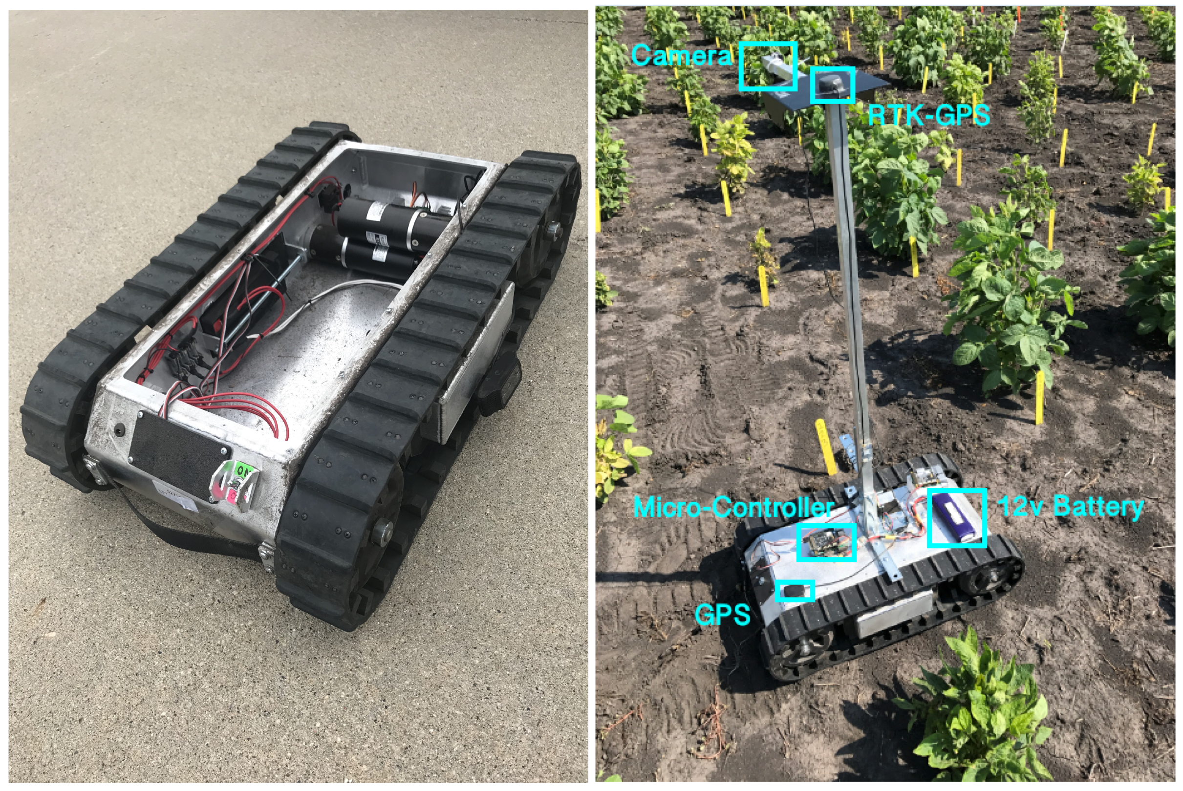
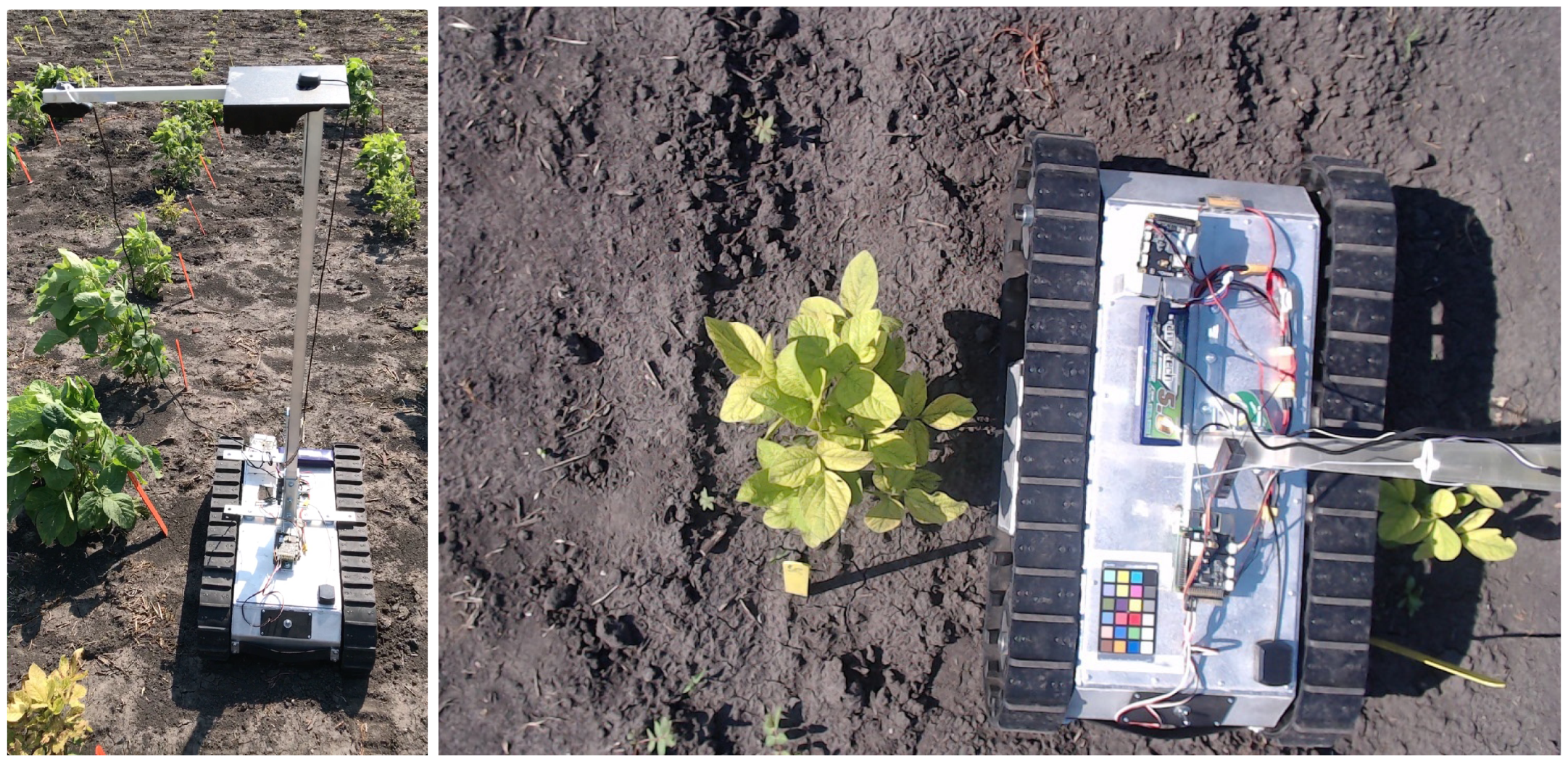
2.1. Robot Configurations

System Requirements for Rover

For phenotyping studies in row crop field, the critical requirement of the robot is that it must fit in between two crop rows and take images without running over the crops. A rover carries a 1 Megapixel Red, Green, Blue (RGB) camera (Logitech, Lausanne, Switzerland) with a 78-degree field of view.

The target soybean plants can grow up to 60 cm and 60 cm wide. To cover a canopy when a rover is next to a soybean plant, we set the camera to the height at 120 cm. Uneven ground and small obstacles should not affect the camera view angle and image quality. The robot has to work in conditions when the ground is damp and muddy. It should maintain high mobility in such conditions. The robot also needs to have enough power to be able to navigate the entire field. It must navigate in the field autonomously with minimum human interaction. However, a human operator should be able to override or stop the robot if necessary. The collected images have to be processed on-board with geo-tag and timestamp, and transmitted to a computer.

Figure 2 shows the rover. The platform is based on a SuperDroid LT2 sold by SuperDroid Robots (Fuquay-Varina, NC, USA). The length of this rover’s base is 67 cm and the width is 42 cm. With a ground clearance of 13 cm, the robot can handle most terrains with its aggressive all terrain treads. With most of its weight on its base, the robot does not tilt or tip easily in the out-door environment. With the height of 120 cm, we are able to mount the imaging sensor anyway in the range of 80 to 120 cm. A pair of tracks driven by the two gear motors can provide a maximum speed of 83 m/min. The height of the system is adjustable between 80 cm and 120 cm. To keep the camera steady to obtain stable images, a 3D gimbal is utilized. The camera always maintains a straight down view of the ground, even when the robot base is tilted caused by uneven ground. Images from on-board camera can be processed efficiently through the strong computing power of Raspberry Pi.

The real-time kinematic (RTK)-GPS antenna, which provides centimeter accuracy, is placed on the top of the mast, near the camera. The regular GPS antenna, which is a back-up, is placed on the robot’s chassis. We do not place the back-up GPS antenna on the mast since it interferes with the RTK-GPS.

2.2. System Architecture

In order to send waypoints and monitor the position and attitude of rovers, we link the ground robots to our ground control station, which is a part of a larger system called Cy-Eye. The rovers communicate with each other through Cy-Eye. The system, shown in Figure 3, is a fully autonomous waypoint based system that consists of a centralized multi-robot ground station that can assign target points for every robot, and generate waypoints on the given field map. Since Cy-Eye system is a fully autonomous GPS waypoint based system, navigation is entirely calculated on-board based on the given waypoints. The centralized ground station sends each robot a list of generated waypoints. After each robot receives the waypoints, the onboard controller with on-board sensors can navigate each robot to follow the given path, and eventually reach the target. We also use this station to initiate commands, and monitor rovers’ status while in operation. It takes in a pre-generated GPS waypoints array for each rover before a human initiates the experiment. Then, it transmits the waypoints to each rover through the Wi-Fi network. Once each rover received the waypoint, an operator can initiate the imaging process. During the process, the operator can view live image and collected data through the graphic user interface. The operator interacts with the robots by viewing and operating the ground station only. The collected data will be saved both on-board and in the ground control station. If emergency occurs, the operator is able to interrupt the process by switching into manual mode. Meanwhile, the ground station is responsible for coordinating the path for multiple robots based on User Datagram Protocol (UDP) protocol for collision avoidance. After two pre-generated waypoints overlap, it will calculate two alternate non-overlapping waypoints and update the original waypoints.

The system uses Wi-Fi network to communicate over the local network or Internet between the ground station and the robots. The protocol is based on Mavlink and UDP.

2.3. Micro-Controller and Sensors

The micro-controller on-board is a Raspberry Pi 3 [15] attached with several sensors, which includes a GPS receiver, barometer, accelerometers, gyroscopes and magnetometers (compass). Additional sensors, for example, a telemetry radio and laser range finder, can also be integrated in this system. Since Raspberry Pi is commonly available and highly scalable both in terms of the type of sensors and the number of sensor nodes [16], it makes the addition of new hardware and software module even more straightforward. The Raspberry Pi’s GPU allows some basic image processing on-board possible. It can be easily mounted on most of the off-the-shelf robot platforms so that an off-the-shelf robot platform can be easily turned into an autonomous robot inside of the Cy-Eye system.

2.4. Middleware and Architecture

Figure 3 shows the diagram of the components and setup of the communication system between robots and ground station. Figure 4 is a high-level view of the Cy-eye architecture. Cy-eye can also incorporate other kinds of vehicles that may have other sensors—for example, a barometer. In this work, only inertial measurement unit (IMU) and GPS (RTK-GPS) are used. In the graphical user interface (GUI) layer, the ground control station is a graphic user interface which integrated with mission control can manage waypoints and data collection points.

2.5. Current Application

This section presents the current application that is implemented on the robot system. We present the informative sampling technique for robots in the field in order to minimize the total distance traveled by the robot for energy saving. Issues involving this waypoint generation process include as to how to pick the next visiting points move in the field, and how to model the environment based on data collected. For tackling such issues, the Gaussian Process (GP) and information-theoretic metric, i.e., Mutual Information (MI) are adopted correspondingly. We first introduce the GP for learning the environment model. Then, we present an assignment and scheduling algorithm for the robots to reach their goal positions. The assignment algorithm minimizes the total distance traveled by the robot, and the scheduling algorithm minimizes the total time taken by the robots to reach their goal based on minimized paths. In the following sections, we present a review of the Gaussian processes and our informative sampling procedure originally proposed in [14]. Section 2.5.1, Section 2.5.2 and Section 2.5.3 are taken verbatim from our previous work in [14].

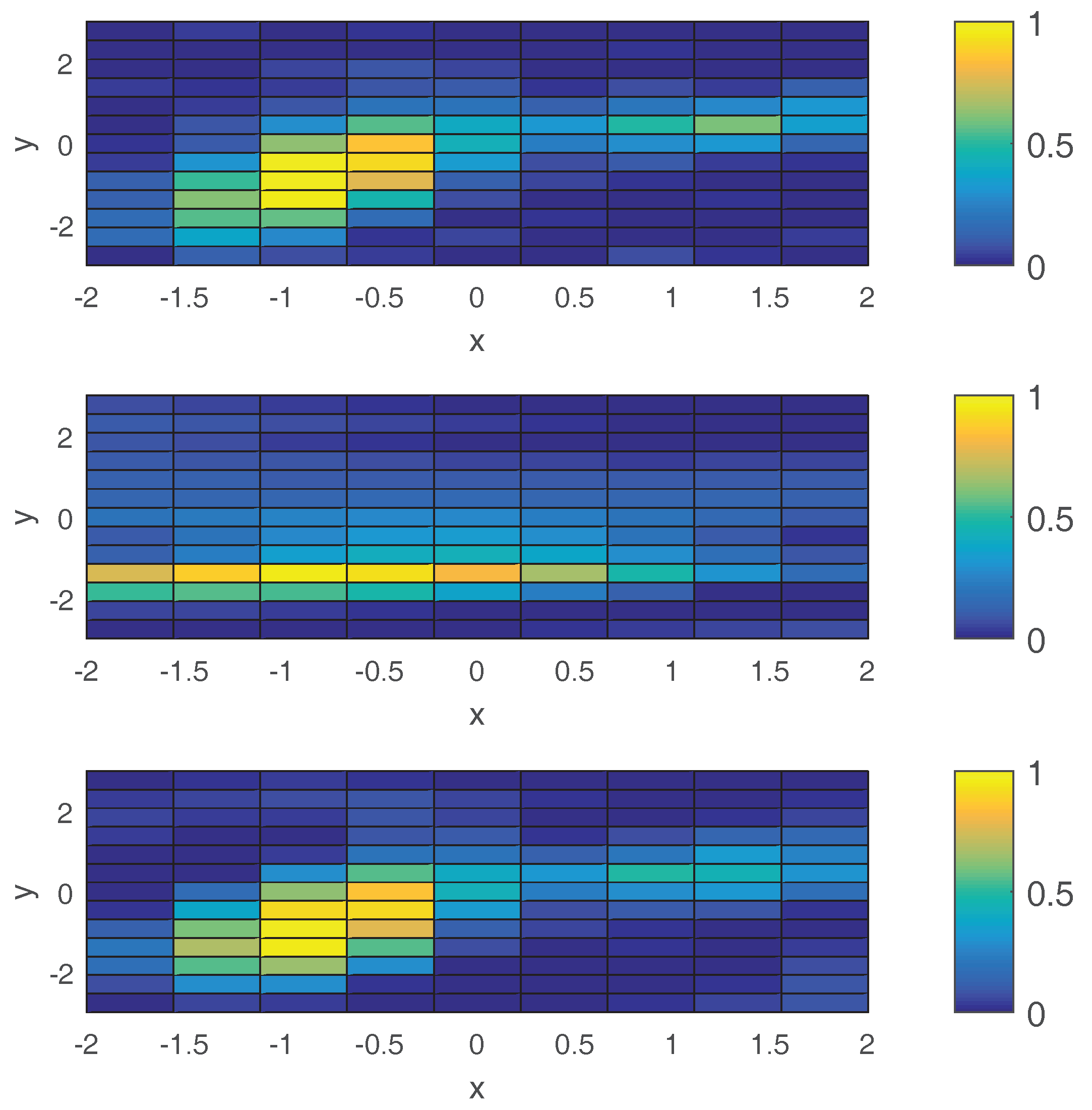
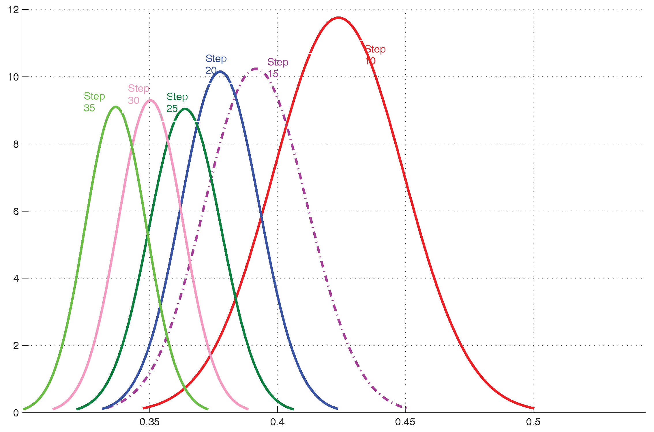
2.5.1. Gaussian Process

A GP is a stochastic process (where random variables are collected from some set) such that any finite subset obtained from the collection has a multivariate Gaussian distribution [17]. GP’s prediction performance depends on the covariance matrix and the input training data set. The covariance matrix is obtained by defining and choosing the prior covariance function which identifies the relationship between two independent data points. The selection of prior covariance function is essentially important for constructing the covariance matrix. In other words, the covariance function defines the nearness or similarity of data points.

We formally describe how to use GP for prediction. Let $S={\{(x^i,y^i)\}}_{i=1}^n,x^i\in {\mathbb{R}}^d,y^i\in \mathbb{R}$ be a training set, where $y^i$ is an observation of Gaussian Process of $f(x)\sim \mathcal{GP}(0,k(x,x^{\prime }))$ at location $x^i$. $k(x,x^{\prime })$ is defined as the covariance function of a real GP of f. We assume a noisy version of measurement of $y^i$ as follows:

$$y^i=f(x^i)+{ϵ}^i,i=1,\cdots ,n,$$

(1)

where ${ϵ}^i$s are i.i.d White noise variables with variance ${\sigma }_n^2$.

Now, let $M={\{(x_{*}^i,y_{*}^i)\}}_{i=1}^m$ be a set of i.i.d. test data set obtained from the same unknown distribution as S. For compactness, let

• $X=[{(x^1)}^T;{(x^2)}^T;\cdots ;{(x^n)}^T]\in {\mathbb{R}}^{n\times d}$ be training input;
• $X_{*}=[{(x_{*}^1)}^T;{(x_{*}^2)}^T;\cdots ;{(x_{*}^m)}^T]\in {\mathbb{R}}^{m\times d}$ be test input;
• ${\mathbf{f}}_{*}=[f(x_{*}^1);f(x_{*}^2);\cdots ;f(x_{*}^m)]\in {\mathbb{R}}^m$ be function values corresponding to test input;
• $\mathbf{y}=[y^1;y^2;\cdots ;y^n]\in {\mathbb{R}}^n$ be training output;

In a GP, the marginal distribution over any subset of inputs must have a joint multivariate Gaussian distribution. Therefore, in this context, for training and test data sets, we have [18]

$$\left[\begin{array}{c}\mathbf{y}\\ {\mathbf{f}}_{*}\end{array}\right]\sim \mathcal{N}\left(0,\left[\begin{array}{cc}K(X,X)+{\sigma }_n^{2}I& K(X,X_{*})\\ K(X_{*},X)& K(X_{*},X_{*})\end{array}\right]\right),$$

(2)

where $K(·,·)$ represent covariance matrices, $K(X,X)\in {\mathbb{R}}^{n\times n},K(X,X_{*})\in {\mathbb{R}}^{n\times m}$, $K(X_{*},X)\in {\mathbb{R}}^{m\times n}$, $K(X_{*},X_{*})\in {\mathbb{R}}^{m\times m}$, I is the $n\times n$ identity matrix.

The last relation follows from that the sums of independent Gaussian random variables is also Gaussian.

Applying the rules for conditioning Gaussians, the predictive equations can be obtained that

$${\mathbf{f}}_{*}|\mathbf{y},X,X_{*}\sim \mathcal{N}({\mu }_{*},{\Sigma }_{*}),$$

(3)

where ${\mu }_{*}\triangleq K(X_{*},X){(K(X,X)+{\sigma }_n^{2}I)}^{-1}\mathbf{y},{\Sigma }_{*}\triangleq K(X_{*},X_{*})-K(X_{*},X){(K(X,X)+{\sigma }_n^{2}I)}^{-1}K(X,X_{*})$.

Based on the discussion above, typically the covariance functions have some free parameters. For this work, we select squared-exponential covariance function as

$$k(p,q)={\sigma }_f^{2}exp(-\frac{1}{2}{(p-q)}^{T}A(p-q))+{\sigma }_n^2{\delta }_{pq},$$

(4)

where $A=diag{(\gamma )}^{-2}$. One can determine the level of correlation by the parameters $\gamma$ for each dimension of p and q. ${\sigma }_f^2$ and ${\sigma }_n^2$ represent the variances of the prediction and noise, respectively. ${\delta }_{pq}$ is the Kronecker delta function that is 1 if $p=q$, while 0, otherwise.

2.5.2. Estimation of Hyperparameters

Based on the above discussion in the last section, we have hyperparameters ${\sigma }_f^2,{\sigma }_n^2,\gamma$ to be estimated. Let $\mathbf{w}\triangleq \{{\sigma }_f^2,{\sigma }_n^2,\gamma \}$. High accuracy of estimation of hyperparameters in the covariance functions can improve the model describing the underlying environment. In this context, we adopt the k-fold cross-validation (CV) [18] via maximum likelihood estimation to solve the problem. As the training data set is only available to be used for estimation, we discuss an extreme case of the k-fold cross-validation (CV) where $k=n$, the number of training points such that leave-one-out cross-validation (LOO-CV) is correspondingly used. The log-likelihood of LOO is as follows:

$$L(X,\mathbf{y},\mathbf{w})\triangleq \sum _{i=1}^n\log p(y^i|X,{\mathbf{y}}_{-i},\mathbf{w}),$$

(5)

where ${\mathbf{y}}_{-i}$ denotes all outputs in the training data set except the one with index i. The explicit form of $\log p(y^i|X,{\mathbf{y}}_{-i},\mathbf{w})$ can be seen in [19]. For obtaining the optimal values of hyperparameters $\mathbf{w}$, we use the gradient descent method as follows:

$$w_j(t+1)=w_j(t)-\alpha (t)g_j(w_j(t)),$$

(6)

where $\alpha (t)$ is the step size, and $g_j(w_j(t))$ is the partial derivative of L at $w_j(t)$ for a j-th hyperparameter set.

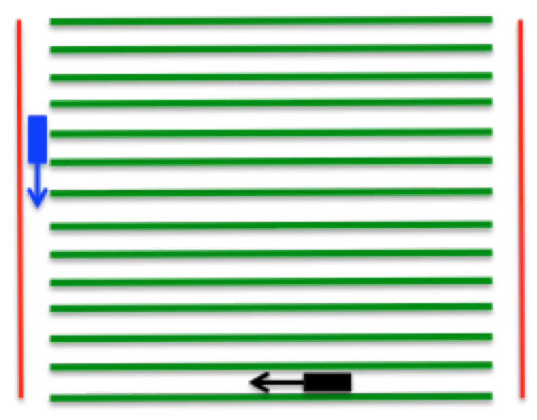
2.5.3. Informative Motions

Robot motions are determined by informative sampling locations, which directly affects the path planning for a robot. For tackling the challenge of future informative sampling locations, a field can be regarded as a discrete grid map in which each grid identifies a possible sampling location. According to the GP, the mean and variance information associated with the measurement at each grid can be predicted accordingly. However, the selection of sampling location is another issue such that an information-theoretic metric for quantifying the information between the sampled locations and unsampled locations is Mutual Information (MI). We formally summarize the MI between two data sets, M and N as follows:

$$I(M;N)=I(N;M)=H(M)-H(M|N),$$

(7)

where $H(M,N),H(M|N)$ are entropy and conditional entropy, respectively, which can be calculated by

$$\begin{array}{c}H(M)=\frac{1}{2}{\log ((2\pi e)}^{\mathcal{B}}|{\Sigma }_{MM}|),\hfill \end{array}$$

(8a)

$$\begin{array}{c}H(M|N)=\frac{1}{2}{\log ((2\pi e)}^{\mathcal{B}}|{\Sigma }_{M|N}|),\hfill \end{array}$$

(8b)

where $\mathcal{B}$ is the size of M. One can calculate the covariance matrix ${\Sigma }_{MM}$ and ${\Sigma }_{M|N}$ via the posterior GP in Equation (3).

In light of the MI metric, to at the highest level obtain the information of true model, it is equivalent to finding new sampling points in the unsampled part that can maximize the MI between sampled locations and unsampled part of the map. We denote by X the entire space (including all grids) and by D a subset of X with a certain size $|D|=n$. Therefore, the set of D includes the most mutual information required for generating the best predictive model. Thus, the following optimization problem is obtained

$$\begin{array}{c}\max I(D;X\setminus D),\hfill \end{array}$$

(9a)

$$\begin{array}{c}\mathrm{s}.\mathrm{t}.D\in \mathcal{D},\hfill \end{array}$$

(9b)

where $\mathcal{D}$ represents all possible combinatorial sets, each of which is of size n.

To solve the optimization problem described above, one can adopt dynamic programming scheme [19] to get the optimal subset $D^{*}$. Algorithm 1 gives the set of points that need to be measured for the next step of the distribution estimation. It should be noted that $D^{*}$ only contains the sampling points that can give the most information for the purpose of best model prediction performance, but does not give us any information about the final path planning. The algorithm for path planning in a farm field is described in the next section.

Algorithm 1 Informative Motions and Nonparametric Learning

1: Input: X, $\mathbf{y}$, k covariance function, $X_{*}$, $m=|X_{*}|$  2: Output: Optimal hyperparameters ${\mathbf{w}}^{*}$  3: Use X, $\mathbf{y}$, k to estimate the hyperparameters in Equation (5)  4: for$z=1:m$do  5:    Divide $X_{*}$ into two parts and customize one part of $X_{*}^z$ and X into N while another part of $X_{*}$ into M  6:    Use posterior GP Equation (3) to calculate the covariance matrices in Equation (8)  7: end for  8: Solve the Equation (9)  9: Include the new data point into X to update GP 10: Repeat Step 3

2.5.4. Path Planning

At each iteration, the assignment of the robots to the goal position needs to be computed by the ground station, and communicated to the robots through the Wi-Fi network. The output of the sampling process is to find the next best points to be visited by the robots. Therefore, the number of the goal points is equal to the number of the robots. At each iteration, a single robot is assigned to a single goal point. A robot that reaches its goal point will wait until all other robots reach their goal points. The next iteration starts only after all robots reach their associated goal points.

In this section, we present an assignment and scheduling algorithm for the robots to reach their goal positions. The assignment algorithm minimizes the total distance traveled by the robot, and the scheduling algorithm minimizes the total time taken by the robots to reach their goal based on minimized paths.

Let us consider a field containing m rows and n columns. The field can be represented as a graph. Each node in the graph is a location of a canopy. We allow only one robot on a node at the same time to avoid collision. Since the distance between any two adjacent columns in the field is not enough for a robot, the robots can only travel in between the rows, which means that they can only switch their rows on the two headland, illustrated in Figure 5, at the end of each row. The nodes in the graph are not adjacent to the nodes above and below them, except the ones on the left and right most columns. The two headlands are called left path and right path. We have k robots and k goal points in the field, $k\le m\times n$. We use a set $\mathbf{A}$ to represent the robots and a set $\mathbf{B}$ to represent the goal points.

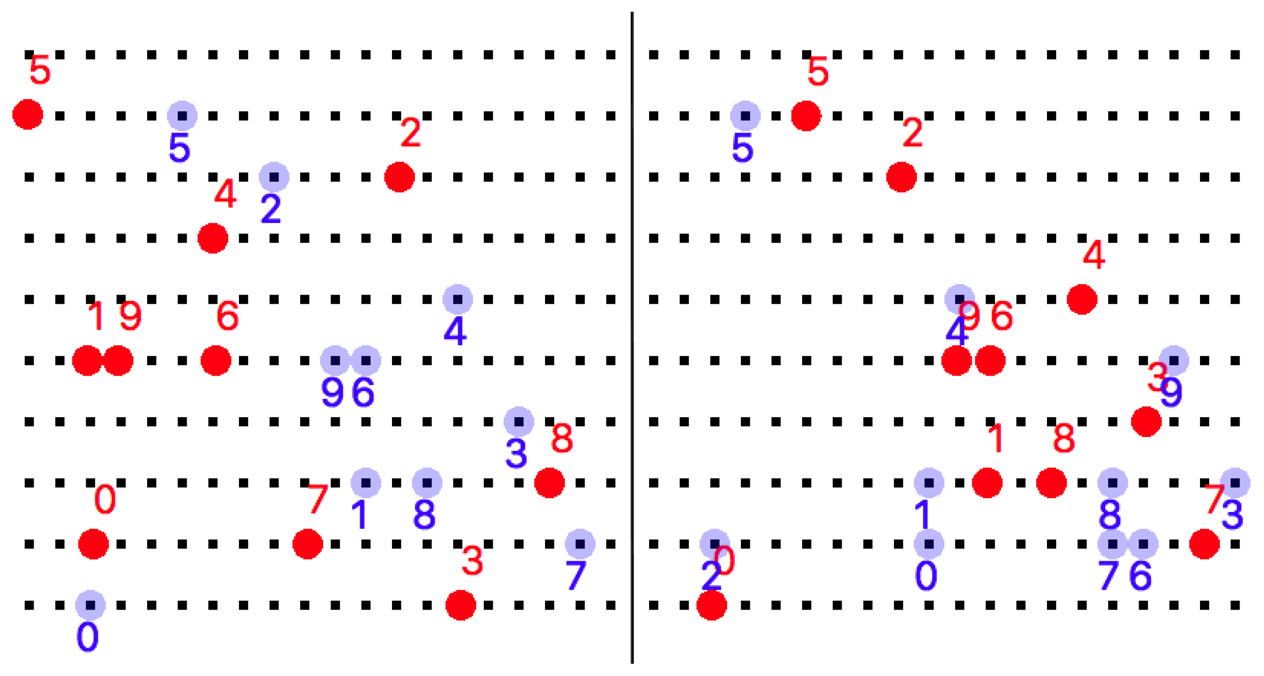
2.5.5. Robot–Target Assignment

For each robot $r_{ij}\in \mathbf{A}$ such that $i\in m,j\in n$, in general, the breadth-first-search algorithm can be used to calculate the distance between the robot $r_{ij}$ and any target $t_{uv}\in \mathbf{B}$ such that $u\in m,v\in n$. However, in the row-crop field, a robot can either run towards the left or right, so it has two possible routes to reach to each target. We select the shorter of the two paths. We use the distances to create a cost matrix for each robots and goal points by using the following algorithm.

With the cost matrix $\mathbf{C}$, we can compute this assignment problem with a well known combinatorial optimization algorithm named Hungarian algorithm [20] in polynomial running time. The total sum of the paths between each robot and its target is minimized.

2.5.6. Tasks Scheduling

The planning algorithm has to ensure that two robots do not collide while they travel on their respective paths. Before we propose our scheduling algorithm, we present the following properties associated with the output of the Hungarian algorithm.

Lemma 1.

In the output of the Hungarian algorithm, two robots do not share any segment of their paths in which they are moving in opposite directions.

Proof. 

If two robots, $r_1$ on the left of $r_2$, can achieve their goal points by moving in opposite directions and intersect at any moment, $r_1$’s path must overlap with $r_2$’s path. The total length of these two paths can be reduced by switching their goal points thereby reducing the total path length by twice the length of the overlapping section. However, this is a contradiction since we assumed that the initial paths minimized the sum of lengths of each path. ☐

Lemma 2.

Consider a row with m robots and n goals such that m robots are only allowed to use the left path.

• If $m>n$, then there is a unique reassignment that allows $m-n$ robots to leave the row, and the remaining n robots to reach their goals without any collision.
• If $n>m$, then there is a unique reassignment that allows $n-m$ robots to enter the row, and the remaining m robots in the row to reach the m goal points without any collision.

The reassignments do not change the sum of path lengths, and do not increase the total time required to complete the task.

Proof. 

 

• Let us consider a labeling of robots $\{r_1,\dots ,r_m\}$ from left to right with the first robot on the left numbered as 1. Goals are labeled from left to right $\{g_1,\dots ,g_n\}$ in a similar manner. Goal $g_n$ is assigned to robot $r_m$, $g_{n-1}$ is assigned to $r_{m-1}$, $g_{n-2}$ is assigned to $r_{m-2}$, and so on, until $g_1$ is assigned to $r_{m-n+1}$. The leftover $m-n$ robots can leave the row without any collision with other robots. This reassignment does not change the sum of the path lengths. Between any two robots being reassigned, the original travel distance for robot $r_i$ and $r_j$ are $d_i$ and $d_j$. The distance between $r_i$ and $r_j$ is d. After reassignment, the traveling distance for $r_i$ is $d_j-d$, and the traveling distance of $R_j$ is $d+d_i$. The total traveling distance is still $d_i+d_j$. Since the total traveling distance remains unchanged, the total time required to complete the task will not increase either.
• Consider the same labeling as in the previous case. Goal $g_n$ is assigned to robot $r_m$, $g_{n-1}$ is assigned to $r_{m-1}$, $g_{n-2}$ is assigned to $r_{m-2}$, and so on, until $g_{n-m+1}$ is assigned to $r_1$. The leftover $n-m$ goals can be taken care of by $n-m$ robots entering from left path without collision. We sort these robots with increasing order by traveling distance to this row. Then, we assign the leftover $n-m$ goals from right to left with the sorted robots. Similarly, this reassignment does not change the sum of path lengths, and does not increase the total time required to complete the task.

 ☐

After reassignment, collision will never happen on rows. For the collision on left and right paths, we propose a strategy that allows the robot that has higher priority to move on to the node that is going to cause collision. The robot that is going to travel more distance has higher priority. Before each robot starts moving towards its next waypoint, if the next waypoint of robot a is the same as the next waypoint of robot b, we let the robot which has lower priority to wait until its next waypoint is not conflicting with the other’s next waypoint. This strategy provides us a collision free scheduling on left and right paths.

By using these strategies, the total traveling distance for all the robots should still be minimized. The total time taken to complete the entire task is the maximum of each individual robot’s task plus the total waiting time caused by collision avoidance.

2.5.7. Time Complexity

The path planning algorithm for minimizing the sum of total traveling distance over all robots is $O(n^3)$, where n is the number of robots. The CostMatrix in Algorithm 2 will take $O(n^2)$ time for constructing the cost matrix. Given the cost matrix, we compute the optimal assignment by Hungarian algorithm in $O(n^3)$ [20] steps. Reassignment process in Lemma 1 takes $O(nlogn)$ since we need to sort all the robots and goal points. Therefore, the entire path planning algorithm is $O(n^3)$.

Algorithm 2 Compute cost matrix given robots and goal points position

Input: Two matrices. $\mathbf{A}$ and $\mathbf{B}$ are robots and goal points location sets Output: Cost matrix $\mathbf{C}$  1: function CostMatrix($\mathbf{A},\mathbf{B}$)  2:  for each $r_{ij}$ do  3:   for each $t_{uv}$ do  4:     ${\mathbf{C}}_{ij}=|i-u|+min(j+v,2n-(j+v)))$  5:   end for  6:  end for      return $\mathbf{C}$  7: end function

3. Results

3.1. Experimental Setup

The experimental plot is 76 cm wide between two connected rows and it has 32 by 39 soybean plants. Figure 6 shows a rover in the field taking images of the canopy and shows the image of the soybean canopy from the overhead camera mounted on the rover. We use a TP-Link AC1750 Wi-Fi router (TP-Link, Shenzhen, China) to serve as the base station to provide the communication between robots and control station. It provides network coverage with a 12v power supply. An RTK-GPS base station, Reach RS, is placed next to the Wi-Fi router to set up our RTK-GPS base station and provide centimeter accuracy. It streams GPS corrections data to the individual robot over the network via Transmission Control Protocol (TCP).

The initial positions of the robots are randomly selected. The set of points that need to be visited by the robots are generated by Algorithm 1. Paths and waypoints for each robot are outputs of the path planning algorithm, described in Section 2.5.4. Since the waypoints for each robot are generated offline from Mission control Figure 4, a human operator with a laptop only needs to start or stop data collection by toggling a button on graphic user interface. Each robot follows the given waypoints and collects data.

3.2. Simulation

In this section, we present the results for the path planning algorithm. In our simulations, we consider a planar environment as our field, and our goal is to estimate the distribution of a scalar field based on adaptive sampling with a group of mobile robots equipped with sensors. The environment and the scalar function can be an agricultural plant area and any phenomena which is distributed spatially, respectively. We consider the scalar function as the distribution of an Iron Deficiency Chlorosis (IDC) value in a farm field.

In order to show the effectiveness of the proposed algorithm, we use synthesized data, generated based on 2D Gaussian distribution. We assume that the intensity of the scalar function is in proportion to the probability density function of a bimodal Gaussian distribution with the following mean and covariance values:

$$\begin{array}{c}\hfill {\mu }_1=\left[\begin{array}{c}-1\\ -1\end{array}\right]{\sigma }_1=\left[\begin{array}{cc}0.2& .3\\ 0.3& 1\end{array}\right]{\mu }_2=\left[\begin{array}{c}1\\ 0.2\end{array}\right]{\sigma }_2=\left[\begin{array}{cc}0.4& .2\\ 0.2& .1\end{array}\right].\end{array}$$

We discretize the field into a grid map, and we associate each grid with a target value which describes the intensity of disease in the plant. Figure 7 shows the distribution of infected plants in the field. We pick $10\%$ of grid points randomly as the training set, and we collect the new data points based on the aforementioned algorithm. We consider three robots (i.e., $n=3$), initially deployed in three different positions in the field. At each step, three sample points are picked, based on Algorithm 1. Each robot is associated with a sample point, based on total distance traveled by the robots, to reach the sample points from the current positions. The evolution of estimation during sampling steps is shown in Figure 7. We compared the error computed from the difference of mean value of the estimated distribution with the truth data. The total number of sampling operations is 30, and Figure 8 shows the histogram of error for these 30 cases while collecting data in different steps. It reveals an average decrease in the estimation error with an increase in the number of iterations.

In the second simulation, we examine the real data, collected from a soybean field. Figure 9 shows the data we collected from the real soybean field by using a rover. The top figure in Figure 9 shows the real distribution of IDC value in the field. The intensity of yellowness in each plant is quantified between 0 and 5 as IDC value. We apply our algorithm on a field, which is 8 by 39 grid points. We pick 30 points randomly as a training set. In order to get a new sample point, we follow the Algorithm 1, and it leads to the informative path.

Figure 10 shows the path planning and assignment for two consecutive iterations. The left part in Figure 10 is the first round of simulation, and the right part is the second round. It shows the assignment for robots and goals. Blue dots indicate goal points and red dots represent robots. The index of robots is on top of red dots, and the index of goal points is below blue dots. The robot will visit the goal point that has the same index number. A video accompanying the submission shows the paths of the robots and the IDC estimates as the iterations progress for several simulation scenarios.

4. Conclusions

In this paper, we presented the design, construction and deployment of a lightweight distributed multi-robot system for row crop phenotypic data collection. Next, we presented an entropy-based informative path planning technique for the robots to navigate in the field. This involves a Gaussian process model for the robots to sample the field to obtain the goal positions of each robot. Next, we proposed a collision-free path planning algorithms for the multiple robots to reach their goal positions in a row crop field. Finally, we presented a deployment scenario for the robots in the field.

As a part of our future work, we plan to modify the rover design to make it suitable for a wider range of phenotyping activities. Another direction of future work is to add aerial vehicles into the multi-robot system to acquire multi-resolution phenotyping capabilities. The system also has a potential role for managements tasks, such as crop monitoring. We plan to explore this in the future.

References

1. Xavier, A.; Hall, B.; Hearst, A.A.; Cherkauer, K.A.; Rainey, K.M. Genetic Architecture of Phenomic-Enabled Canopy Coverage in Glycine max. Genetics 2017, 206, 1081–1089. [Google Scholar] [CrossRef] [PubMed] [Green Version]
2. Naik, H.S.; Zhang, J.; Lofquist, A.; Assefa, T.; Sarkar, S.; Ackerman, D.; Singh, A.; Singh, A.K.; Ganapathysubramanian, B. A real-time phenotyping framework using machine learning for plant stress severity rating in soybean. Plant Methods 2017, 13, 23. [Google Scholar] [CrossRef] [PubMed]
3. Bai, G.; Ge, Y.; Hussain, W.; Baenziger, P.S.; Graef, G. A multi-sensor system for high throughput field phenotyping in soybean and wheat breeding. Comput. Electron. Agric. 2016, 128, 181–192. [Google Scholar] [CrossRef]
4. Shi, Y.; Thomasson, J.A.; Murray, S.C.; Pugh, N.A.; Rooney, W.L.; Shafian, S.; Rajan, N.; Rouze, G.; Morgan, C.L.; Neely, H.L.; et al. Unmanned aerial vehicles for high-throughput phenotyping and agronomic research. PloS ONE 2016, 11, e0159781. [Google Scholar] [CrossRef] [PubMed]
5. Tattaris, M.; Reynolds, M.P.; Chapman, S.C. A Direct Comparison of Remote Sensing Approaches for High-Throughput Phenotyping in Plant Breeding. Front. Plant Sci. 2016, 7, 1131. [Google Scholar] [CrossRef] [PubMed]
6. Ruckelshausen, A.; Biber, P.; Dorna, M.; Gremmes, H.; Klose, R.; Linz, A.; Rahe, F.; Resch, R.; Thiel, M.; Trautz, D.; et al. BoniRob: an autonomous field robot platform for individual plant phenotyping. In Precision Agriculture ’09; Wageningen Academic Publishers: Wageningen, The Netherlands, 2009. [Google Scholar]
7. Gonzalez-de Santos, P.; Ribeiro, A.; Fernandez-Quintanilla, C.; Lopez-Granados, F.; Brandstoetter, M.; Tomic, S.; Pedrazzi, S.; Peruzzi, A.; Pajares, G.; Kaplanis, G.; et al. Fleets of robots for environmentally-safe pest control in agriculture. Precis. Agric. 2017, 18, 574–614. [Google Scholar] [CrossRef]
8. Bawden, O.; Ball, D.; Kulk, J.; Perez, T.; Russell, R. A lightweight, modular robotic vehicle for the sustainable intensification of agriculture. In Proceedings of the Australian Conference on Robotics and Automation (ACRA 2014), Melbourne, Australia, 2–4 December 2014. [Google Scholar]
9. Grimstad, L.; From, P.J. The Thorvald II agricultural robotic system. Robotics 2017, 6, 24. [Google Scholar] [CrossRef]
10. Fernandez, M.G.S.; Bao, Y.; Tang, L.; Schnable, P.S. A high-throughput, field-based phenotyping technology for tall biomass crops. Plant Phys. 2017. [Google Scholar] [CrossRef] [PubMed]
11. Arbo, M.H.; Utstumo, T.; Brekke, E.F.; Gravdahl, J.T. Unscented Multi-Point Smoother for Fusion of Delayed Displacement Measurements: Application to Agricultural Robots. Model. Identif. Control 2017, 38, 1–9. [Google Scholar] [CrossRef] [Green Version]
12. Batey, T. Soil compaction and soil management—A review. Soil Use Manag. 2009, 25, 335–345. [Google Scholar] [CrossRef]
13. Nawaz, M.F.; Bourrie, G.; Trolard, F. Soil compaction impact and modelling. A review. Agron. Sustain. Dev. 2013, 33, 291–309. [Google Scholar] [CrossRef]
14. Saha, H.; Gao, T.; Emadi, H.; Jiang, Z.; Singh, A.; Ganapathysubramanian, B.; Sarkar, S.; Singh, A.; Bhattacharya, S. Autonomous Mobile Sensing Platform for Spatio-Temporal Plant Phenotyping. In Proceedings of the ASME 2017 Dynamic Systems and Control Conference, Tysons, VA, USA, 11–13 October 2017; p. V002T21A005. [Google Scholar]
15. Pi, R. Raspberry Pi Model B, 2015. Available online: http://www.meccanismocomplesso.org (accessed on 30 July 2018).
16. Ferdoush, S.; Li, X. Wireless sensor network system design using Raspberry Pi and Arduino for environmental monitoring applications. Procedia Comput. Sci. 2014, 34, 103–110. [Google Scholar] [CrossRef]
17. Williams, C.K.; Rasmussen, C.E. Gaussian Processes for Machine Learning; MIT Press: Cambridge, MA, USA, 2006. [Google Scholar]
18. Rasmussen, C.E. Gaussian processes for machine learning. J. Mach. Learn. Res. 2010, 11, 3011–3015. [Google Scholar]
19. Ma, K.C.; Liu, L.; Sukhatme, G.S. Informative planning and online learning with sparse gaussian processes. In Proceedings of the 2017 IEEE International Conference on Robotics and Automation (ICRA), Singapore, 29 May–3 June 2017; pp. 4292–4298. [Google Scholar]
20. Kuhn, H.W. The Hungarian method for the assignment problem. Nav. Res. Logist. Quart. 1955, 2, 83–97. [Google Scholar] [CrossRef] [Green Version]
Figure 1. Deployment strategy of robotic phenotyping system.
Robotics 07 00061 g001
Figure 2. The figure on the left shows the rover. The figure on the right shows the rover in the field taking images of the canopy.
Robotics 07 00061 g002
Figure 3. Architecture of Cy-Eye.
Robotics 07 00061 g003
Figure 4. Robot architecture.
Robotics 07 00061 g004
Figure 5. Two robots moving in the field. The black robot moving towards the left in between two rows. The blue robot is moving downward on the left headland.
Robotics 07 00061 g005
Figure 6. Image of the soybean canopy from the overhead camera mounted on the rover.
Robotics 07 00061 g006
Figure 7. The plot at the top shows the heat-map of a scalar function between 0 and 1, in a planar field. The middle plot shows the initial distribution of the estimation. The bottom plot is the final distribution estimation after informative sampling.
Robotics 07 00061 g007
Figure 8. Histogram of error.
Robotics 07 00061 g008
Figure 9. The plot on the top shows the heat-map of IDC values, scaled between 0 and 5, in a soybean field. The plot in the middle shows the initial distribution estimation. The bottom figure is the final distribution estimation after informative sampling.
Robotics 07 00061 g009
Figure 10. Two consecutive path planning algorithm simulation. The image on the left is when t = i , and the image on the right is when t = i + 1 . Red dots indicate the position of the robots. Blue dots represent the location of the sample points.
Robotics 07 00061 g010