Decomposing US Money Supply Changes since the Financial Crisis

Abstract

In response to the financial crisis of 2008, the Federal Reserve radically increased the monetary base. Banks responded by increasing excess reserves rather than increasing bank loans, and the public responded with a substantial flight to liquidity in the form of currency and demand deposits. As a result, the money-supply multipliers substantially decreased, so that the actual money supply measures grew more moderately than the base. The sustained multiplier-collapse spawned reexamination of monetary versus fiscal theories of price-level determination. This paper, however, presents decompositions of the money-multiplier collapse into changes in the currency-to-deposit ratios, and changes in the reserve-to-deposit ratio. By doing so, possible near-term increases in the multipliers are simulated so that the possibility of either full or partial restoration to their pre-crisis levels is assessed. Policy possibilities for controlling the money supply over various horizons follow. This analysis illustrates the Federal Reserve’s exit dilemma that results from its financial-crisis policy.

1. Introduction

One conventional view of Federal Reserve (the Fed) policy during the post 2008 financial crisis is that its open-market operations were merely “pushing on the string of a liquidity trap.” In fact, the Fed began lowering its Federal Funds rate target in September 2007. Over the following year, it lowered this target rate from 5.25 percent to 2 percent. Post the financial panic of mid-September, 2008 (the collapse of Lehman Brothers), it further dropped the target rate to approximately 0.25 percent. As indicated by Blinder [1], it became apparent at this time that lowering “liquidity premiums,” and “risk premiums” became the essentially needed task of monetary policy.1 Since the riskless overnight rate became essentially zero, the Fed needed to more directly flatten both the risk-free yield curve and the risk-structure of yields.

The policies the Fed utilized to accomplish this narrowing of spreads has been termed quantitative easing, i.e., QEI was initiated in late 2008, QEII in late 2009, and operation twist in 2011. Essentially this latter policy involved purchasing very large amounts of targeted securities: i.e., mortgage-backed securities, agency debt securities (which allowed agencies to further support the mortgage market), commercial paper, money-market mutual fund securities, and medium and longer-term Treasury bonds. Essentially this quantitative easing involved the Fed directly purchasing one of the risky or less-liquid assets from financial markets, and paying for these purchases by either liquidating its portfolio of T-bills or increasing the monetary base. The former involved no net increase in the Fed’s assets, but the latter resulted in an increase. Total Fed assets skyrocketed from approximately $0.91 trillion on September 3, 2008, to approximately $2.2 trillion on November 12, 2008. Almost all of this increase was absorbed by the banking system as excess reserves which increased from approximately $2 billion in August, 2008, to $0.77 trillion in December, 2008.

The early stages of the quantitative easing policy was “ad hoc, reactive and institution based” ([1], p. 469). Initially, in late 2008, the Fed developed its policy “on the fly,” often on short-term notice, by acquiring assets as a result of rescue operations, e.g., the Maiden Lane MBS (Mortgage-Backed Securities) portfolio from AIG. The problem of this early financial-crisis period, however, was that the resulting increase in the monetary base was not loaned by the banking system. The increase remained as excess reserves, as shown in Table 1a. As a result, the money multiplier collapsed, also shown in Table 1a. Because of radical increase in the monetary base, however, on net the money supply did increase at relatively modest rates during this period and up to the present time (March of 2013). These rates are also shown in Table 1b. As bank intermediaries ceased their loan function, the economy sank into the Great Recession. The problems posed for future Fed policy concerns what might happen when banks resume their loan activity, especially with this very large existing monetary base.

In addition to the problem with excess reserves, the public responded to the financial crisis with a substantial flight to liquidity in the form of currency and demand deposits. As a result, the money-supply multipliers substantially decreased.2 The monetary policy dilemma the Fed must now confront is that if the money multipliers rapidly increase towards their pre-crisis levels then a radical increase in the money supply and consequent significant inflation will surely result. This is a problematic fact that looms over Fed policy, a problem examined here.

Table 1. a. Money Supply Components (in $billions except for Mult. 1) ¹. b. Annualized Growth Rates in M1, 2008 to 2011.

a.

	3/2006	3/2008	3/2010	3/2012
M1	$1,383.4	$1,387.7	$1,712.3	$2,220.7
Mult. 1	1.734	1.683	0.825	0.838
Monetary Base 2	$798.0	$824.4	$2,074.6	$2,650.4
Total Reserves	$43.9	$45.0	$1,186.9	$1,608.0
Excess Reserves	$1.5	$2.6	$1,120.3	$1,509.7
Required Reserves	$42.4	$42.3	$65.6	$98.3

a.

	3/2006	3/2008	3/2010	3/2012
M1	$1,383.4	$1,387.7	$1,712.3	$2,220.7
Mult. 1	1.734	1.683	0.825	0.838
Monetary Base 2	$798.0	$824.4	$2,074.6	$2,650.4
Total Reserves	$43.9	$45.0	$1,186.9	$1,608.0
Excess Reserves	$1.5	$2.6	$1,120.3	$1,509.7
Required Reserves	$42.4	$42.3	$65.6	$98.3

b.

Year	Annualized M1 Growth Rates
2008	14.12%
2009	7.67%
2010	10.52%
2011	18.09%

¹ See [6] for sources of money supply data, “Series H.3.” ² The “Monetary Base” consists of bank reserves plus currency in the hands of the public.

b.

Year	Annualized M1 Growth Rates
2008	14.12%
2009	7.67%
2010	10.52%
2011	18.09%

¹ See [6] for sources of money supply data, “Series H.3.” ² The “Monetary Base” consists of bank reserves plus currency in the hands of the public.

Sims [7] argues that the great expansion of the Fed’s balance sheet over the last four years need not generate inflationary pressure since paying interest on these excess reserves gives little incentive for banks to loan. Sims does acknowledge, however, that if the Fed needs to raise these rates on reserves, then since US Treasuries and reserves are substitutes on the banks’ balance sheets, the yields on Treasuries will also increase. Hence there is a new interaction between fiscal and monetary policies. Sims does not acknowledge, however, that the rate paid on these bank reserves becomes their growth rate, ceteris paribus. Consequently, as an instrument of monetary policy, paying interest on excess reserves merely delays the inevitable problem that they must be eventually liquidated either through bank loans or monetary policy actions.

This paper presents decompositions of the growth in M1 and the changes in its multiplier, a decomposition that allows insights into the future course and effects of monetary policy. For example, any increase in the M1 multiplier that results from a switch from excess reserves to bank loans will have a different effect on the economy than an increase in the multiplier caused by a reduction in currency held by the public. Consequently we decompose changes in the money multiplier, as they have occurred since the onset of the financial crisis, into various factors such as the changes in the currency-to-deposit ratio, changes in the other-checkable-deposit ratio, and changes in the total-reserve-to-deposit ratio. In light of this decomposition, possible near-term increases in the multiplier are simulated so that the possibility of full or partial restoration to its pre-crisis level is assessed. This examination includes explorations of the options the Fed has for handling the excess reserves, and simulations of the money supply expansion process. This simulation analysis further illustrates the Fed’s exit dilemma from its financial-crisis policy.

2. Options for the Fed’s Exit Strategy

The Fed currently (3/2013) holds $1.19 trillion in MBS and Agency Debt Securities, and $1.82 trillion in US Treasury securities.3 A significant problem concerns the liquidation of its holdings of securities while also reducing excess bank reserves, which are approximately $1.8 trillion. These reserves are eligible for loans by banks, and if they are loaned quickly, then inflation will surely result. The simulations provided in the next section help to analyze this problem.

Bernanke [1] stated the options the Fed has for a planned “exit strategy”.

• Redeeming or selling securities in conventional (traditional) open-market operations.
• Passively redeeming MBS, agency debt, and Treasuries as they mature, and not purchasing replacement securities.
• Selling reverse repurchase agreements so as to maintain the prices of these securities.
• Increasing the interest rates it pays on reserve deposits so that banks will not loan these reserves out.
• Offer to depository institutions term-deposits which … could not be counted as reserves.” (p. 8)

With respect to the first option, i.e., the selling of securities in conventional open-market operations, we note that because the Fed’s current portfolio is largely longer-term Treasuries and mortgage-backed securities, both of which the Fed acquired to support different segments of capital markets, it must be reluctant to sell these securities at least until after these particular market segments have experienced robust and sustained restoration. Over the previous three years, the Fed has not used open market operations to reduce the monetary base, but if markets warrant, this is certainly the most viable policy option. The Fed did sell the Maiden Lane MBS portfolio during 2011 although it sterilized this sale through the purchase of long-term Treasuries.

With respect to the second Fed option, i.e., the passive allowance of redemption of securities without repurchasing similar securities, we note that post September, 2011, the Fed did the opposite by purchasing similar replacements for those that matured and were redeemed. This action maintained the monetary base rather than allowing it to contract. Still, this policy option has potential for decreasing the base if and when credit conditions warrant.

With respect to the third option, the selling of reverse-repurchase agreements, note that if this option is utilized, it would allow the Fed to maintain the prices of securities involved in that if market conditions deteriorate for the securities the Fed sells on a repo basis, then the repurchase option could restore the price level. Of course, since the monetary base has been relatively stable over 2010 to early 2013, this option remains to be utilized to any substantial amount.

With respect to the fourth option, i.e., the payment of interest on reserve deposits, this can only be an effective option when credit conditions are poor, and the interest rates the Fed must pay are low, such as its current 0.25 percent (Blinder [1] examines this difficulty). It must be kept in mind that the interest paid on these reserves becomes an addition to the monetary base, so that as an instrument for controlling the base, this could only work when competitive rates are low. If credit conditions heat up and interest rates rise so that banks could earn perhaps 6 percent or higher on loans, then for the Fed to pay higher than this to keep banks from loaning out their excess reserves would mean substantial increases in the very base its controls are aimed at. This only delays and exacerbates the inevitable problem.

The fifth option, the conversion of excess reserves into time deposits with appropriate interest paid, has the same problem as the fourth option. The interest is added to the same reserves that are to be controlled, so that the problem of liquidating excess reserves is exacerbated and merely delayed.

It is interesting to note that Bernanke did not mention increasing reserve requirements, which certainly appears to be a viable option under the current circumstances of extremely high excess reserves. It appears that increasing the required-reserve-to-deposit ratio would absorb at least a portion of the excess, and as a consequence, ameliorate a portion of this problem. The possible reasons why this might not be considered as a current option include:

• The Fed might fear that the announcement effects of changes in reserve requirements could mistakenly indicate an over tightening of credit when conditions do not warrant this reaction.
• An increase in reserve requirements might have differential impacts on banks where those that have already begun to loan, something the Fed surely wants, are hurt relative to those who have preferred to sit on their current position.
• Note that Chairman Bernanke is a scholar of the Great Depression of the 1930s (see Bernanke [8], and [9]), when reserve requirements were doubled over a six month period in 1936, and credit markets collapsed so as to cause a second massive decline in real output during the Great Depression (the first being between 1930 and 1933). Surely the Fed is likely to be reluctant to repeat this historical experience.4

After considering these three reasons, only moderate increases in the required reserve ratio are acceptable, an increase which we do consider in the simulations presented below.

If the loan markets do heat up, then the money multiplier will rise rapidly towards its pre-crisis level, and the Fed will have to reverse its quantitative easing policy, and reduce the monetary base. To not do so would result in substantial increases in the money supply, and likely consequent inflation. In order to indicate the extent of the problem, and the tight path the Fed must follow to manage and avoid this inflation, below we provide simulations of changes in the money-multiplier, and the monetary base.

3. Multiplier Decomposition

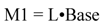
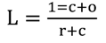
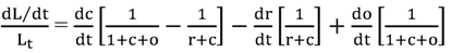
The money supply process for M1 is described by equation (1) where L is the money multiplier as given by (2), and Base consists of the reserves of the banking system plus currency in the hands of the public.5

(1)

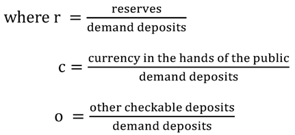
(2)

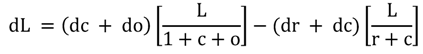
In equation (2), L is a simplified money multiplier in that the variable “reserves” includes both required and excess reserves, and M1 includes currency in the hands of the public, plus demand deposits, plus other checkable deposits.6 Equation (3) gives the total differential of (2), and (4) gives this differential in the form of instantaneous percentage changes, i.e., dln(L)/dt where t is time.

(3)

(4)

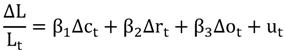
Equation (4) suggests the time-series model (5) where ∆L, ∆r, ∆c and ∆o are all changes through time, and u_t is a random error term that reflects any imperfections in the simplified multiplier measurements.

(5)

Model equation (5) can be estimated from time-series data. This allows the decomposition of the money multiplier into changes in the currency ratio (∆c), changes in the reserve ratio (∆r), and changes in the other-checkable-deposits ratio (∆o).

4. Empirical Estimation

4.1. Data Set Analyzed

To estimate equation (5), monthly data for M1, the Monetary Base, and Total Reserves were gathered from series H.3 [6], 12/2006 to 3/2012, seventy-five monthly observations. All data was Not Seasonally Adjusted, and the reserve data was also not adjusted for required reserves. Similar monthly data for Currency in the Hands of the Public, and Demand Deposits, were gathered from series H.6, Not Seasonally Adjusted for the same months. Table 2a presents the basic statistics for the data analyzed. Table 2b presents the means and standard deviations for the relevant variables as measured over the time period 8/2008 to 3/2012.

Table 2. a. Basic Statistics for M1 and Its Multiplier. b. Mean Averages and Standard Deviations Over Period 8/2008 to 3/2012.

a.

Month	M1 1	Base 1	Total Reserves 1	Demand Deposits 1	Currency 2	Other Check.3	Mult. 4	r	c	o
3/2012	$2,239.2	$2,654.54	$1,606.48	$771.8	$1,033.1	$430.2	0.8435	2.08	1.34	0.56
8/2008	$1,400.9	$847.30	$44.13	$305.6	$774.8	$305.7	1.6745	0.14	2.54	1.00
%∆ 5	+59.83	+213.29	3,540.34	+152.55	+33.23	40.73	−48.98	1,344	−7.24	−44.28

a.

Month	M1 1	Base 1	Total Reserves 1	Demand Deposits 1	Currency 2	Other Check.3	Mult. 4	r	c	o
3/2012	$2,239.2	$2,654.54	$1,606.48	$771.8	$1,033.1	$430.2	0.8435	2.08	1.34	0.56
8/2008	$1,400.9	$847.30	$44.13	$305.6	$774.8	$305.7	1.6745	0.14	2.54	1.00
%∆ 5	+59.83	+213.29	3,540.34	+152.55	+33.23	40.73	−48.98	1,344	−7.24	−44.28

b.

	M1	Base	Total Reserves	Demand Deposits	Currency	Multiplier	r	c	o
Means	$1,617.9	$1,526.4	$674.7	$426.6	$836.9	1.2343	1.314	2.0877	0.8642
S.D.	265.8	694.9	618.3	142.3	88.4	0.4066	1.080	0.3945	0.1568

¹ Denoted in $billions; ² “Currency in the Hands of the Public” in $billions; ³ “Other Checkable Deposits” in $billions; ⁴ Multiplier = M1/Base = L in equation (2); ⁵ %∆ is the percentage change over the period 8/2008 through 3/2012.

b.

	M1	Base	Total Reserves	Demand Deposits	Currency	Multiplier	r	c	o
Means	$1,617.9	$1,526.4	$674.7	$426.6	$836.9	1.2343	1.314	2.0877	0.8642
S.D.	265.8	694.9	618.3	142.3	88.4	0.4066	1.080	0.3945	0.1568

¹ Denoted in $billions; ² “Currency in the Hands of the Public” in $billions; ³ “Other Checkable Deposits” in $billions; ⁴ Multiplier = M1/Base = L in equation (2); ⁵ %∆ is the percentage change over the period 8/2008 through 3/2012.

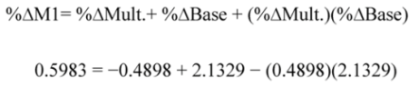
The statistics show that although there was a flight to currency during the period 8/2008 to 3/2012, the coincident increase in demand deposits was greater so that the currency-to-deposit ratio actually declined. The reserves-to-deposit ratio, however, increased by approximately 1,345 percent, so that this change more than counteracted the effects on the multiplier of a decrease in c, and as a result, the net effect decreased the multiplier. Equation (5) indicates that the effects of ∆c on the multiplier must be less than the effects of ∆r, and the large positive magnitude of ∆r must account for the almost 50 percent decline in the multiplier over the 2008–2012 period.

Table 2a also shows that the Base increased substantially (213 percent) over the 8/2008 to 3/2012 period. This Base increase offset the Multiplier decline to result in an increase in M1 by 60 percent over this period. Equation (6) presents the decomposition of this decline in M1.

(6)

Table 3 presents an OLS (Ordinary Least-Squares) estimate of equation (5), the percentage change in the multiplier, with the constant-intercept term suppressed in this regression.

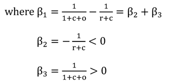
Since the OLS estimation of equation (5) indicates that both β₁ and β₃ are insignificantly different from zero, then equation (7) was also estimated. The results are reported in Table 4. The F-ratio for inclusion of ∆c is F = 0.67. As a result, the OLS analysis that the hypothesis that ∆c and ∆o contribute explanatory power to the model is rejected at 99% significance level, i.e., the joint hypothesis that β₁ = β₃ = 0 cannot be rejected.

(7)

Table 3. OLS Estimates of Model Equation (5) ¹.

Coefficient	OLS Estimate	S.E. of Est.	t-statistic	p-value
β1	−0.0453	0.0737	−0.62	0.46
β2	−0.2492	0.0252	−9.90	0.000
β3	+0.2701	0.2077	+1.30	0.198
R2 = 0.6066	F = 36.50	p = 0.000		0.000

¹ The constant-intercept term was suppressed in the OLS estimation.

Table 3. OLS Estimates of Model Equation (5) ¹.

Coefficient	OLS Estimate	S.E. of Est.	t-statistic	p-value
β1	−0.0453	0.0737	−0.62	0.46
β2	−0.2492	0.0252	−9.90	0.000
β3	+0.2701	0.2077	+1.30	0.198
R2 = 0.6066	F = 36.50	p = 0.000		0.000

¹ The constant-intercept term was suppressed in the OLS estimation.

Table 4. OLS Estimates of Model Equation (7) ¹.

Coefficient	OLS Estimate	S.E. of Est.	t-statistic	p-value
β2	−0.2251	0.0247	−10.32	0.000
R2	0.5969

¹ The intercept term is suppressed in this OLS estimation.

Table 4. OLS Estimates of Model Equation (7) ¹.

Coefficient	OLS Estimate	S.E. of Est.	t-statistic	p-value
β2	−0.2251	0.0247	−10.32	0.000
R2	0.5969

¹ The intercept term is suppressed in this OLS estimation.

4.2. Calculated Effects of c, o and r on the Multiplier

The OLS empirical analysis indicates that changes in the currency ratio ∆c, and the other-checkable-deposits ratio ∆o, have little to no effects on the money multiplier, i.e., β₁ ≈ β₃ ≈ 0. Table 5, however, presents descriptive statistics of β₁, β₂, and β₃ as based upon monthly calculations using the formulae of equation (5) and monthly calculations of c, r and o. The mean estimates align closely with the OLS estimates, but the range for each coefficient is fairly wide. For example, the minimum value for β₁ is −0.18 which indicates that ∆c might have had a significant inverse impact on the multiplier over some sub-period, although in total over the entire period investigated, its effects often have little to no impact.

Table 5. Descriptive Statistics Using Monthly Observations from Equation (5), 1/2006 to 3/2012.

Coefficient	Mean	SE Mean	t-statistic	Minimum	Maximum	Range
β1	−0.0515	0.0116	−4.44	−0.1845	+0.0793	0.2638
β2	−0.3099	0.0082	−37.79	−0.4212	−0.2078	0.2134
β3	+0.2584	0.0046	+56.17	+0.2090	+0.3552	0.1461

Table 5. Descriptive Statistics Using Monthly Observations from Equation (5), 1/2006 to 3/2012.

Coefficient	Mean	SE Mean	t-statistic	Minimum	Maximum	Range
β1	−0.0515	0.0116	−4.44	−0.1845	+0.0793	0.2638
β2	−0.3099	0.0082	−37.79	−0.4212	−0.2078	0.2134
β3	+0.2584	0.0046	+56.17	+0.2090	+0.3552	0.1461

The effects of changes in the total reserve ratio (∆r) clearly had an impact of substantial size. The mean of the calculations of β₂ shows the largest absolute magnitude among the coefficients; ∆r clearly had a substantial inverse effect on the multiplier. The impact of ∆o on the multiplier is clearly positive; an increase in “other-checkable-deposits” as a ratio of demand deposits increases the multiplier. In addition, the t-statistics shown in Table 5 indicates that the means statistics for β₁, β₂, and β₃ are significantly different from 0 for each. Also, the ranges for β₂ and β₃ are entirely positive, although the range for β₁ includes both negative and positive values. Also, at the means for these coefficients we do have β₁ = β₂ + β₃ as established by (5).

We conclude, from the combination of the mean and OLS analysis that increases in the total-reserve ratio and increases in the other-checkable-deposits ratio have effects of similar, but opposite in direction, magnitudes on the money multiplier. Changes in the currency ratio have a smaller, but occasionally significant magnitude, effect.

5. Implications for Monetary Policy

The estimate of equation (5) has interesting implications for the future of monetary policy in that it allows an estimation of the change in the money-multiplier given a return to normal levels with respect to excess reserves. Table 6 presents the percentage changes in the multiplier (L) given returns of r, o and c to their former levels on 8/2008. Table 2a shows their levels on the selected dates of 8/2008 and 3/2012, and the time difference values of ∆r = +1.94, ∆c = −1.20, and ∆o = −0.44 as calculated. These reversals are presented in Table 6. Using the mean values for β₁, β₂, and β₃ presented on Table 5, the percentage changes in L are computed and presented. As shown, if all three variables (r, c and o) return to their pre-financial crisis levels, the multiplier will increase by 65.31 percent.

Table 6. Impacts on %∆L of Restoration of r, c and o to 8/2008 Levels.

Variable	∆L/L	%∆L
∆r = −1.94	∆r(Mean β2) = (−1.94)(−0.3099) = +0.6012	60.12%
∆c = +1.20	∆c(Mean β1) = (+1.20)(−0.0515) = −0.0618	−6.18%
∆o = +0.44	∆o(Mean β3) = (+0.44)(+.2584) = +0.1137	11.37%
	Total = +0.6531	Total = 65.31%

Table 6. Impacts on %∆L of Restoration of r, c and o to 8/2008 Levels.

Variable	∆L/L	%∆L
∆r = −1.94	∆r(Mean β2) = (−1.94)(−0.3099) = +0.6012	60.12%
∆c = +1.20	∆c(Mean β1) = (+1.20)(−0.0515) = −0.0618	−6.18%
∆o = +0.44	∆o(Mean β3) = (+0.44)(+.2584) = +0.1137	11.37%
	Total = +0.6531	Total = 65.31%

The flight to liquidity involving the increase in currency ratio (c) and other-checkable-deposits ratio (o), add only slightly more than 5% to the multiplier, but the reduction in the total reserves-to-deposit ratio to its pre-crisis level increases the multiplier slightly more than 60 percent.

During 2006, and before the onset of the financial crisis, the reserve-to-deposit ratio hovered about its approximate long-term average of 0.14. Post the crisis, and because of the radical increase in the excess reserves, this reserve-to-deposit ratio has hovered above 2.0. A return to “normality” of a ratio of 0.14, i.e., if the banking system loans the excess reserves as is typically the case during economic growth periods, then the money supply increases by approximately 60 percent assuming no change in the monetary base. It should be obvious that a 60 percent increase in the money supply M1 over a period of even 5 years or less is unacceptable for the course of Federal Reserve monetary policy. A 60 percent increase over a period of even a decade would likely be unacceptably large because of consequent inflation.

6. Simulated Monetary Results under Various Fed Options

The purpose of quantitative easing is to purchase private sector assets by a substantial amount so as to reduce term- and risk-premiums. Anderson, et al. [2] examined these monetary policies across international central banks. They point out that quantitative easing policies have been effective only when the central banks are credible with respect to unwinding their balance-sheet adjustments so as to prevent consequent inflation. Bullard [3] reinforces the importance of this credibility for Fed policy with respect to the current need for unwinding excess reserves. Note that not all economic analysts find the Fed’s policy as credible. (See Meltzer [15] as an example.) Its credibility depends upon two characteristics:

• The central bank’s political authority (perhaps independence from other governmental influence) and willingness to handle the inflation problem.
• The central bank’s power to resolve the problem.

The latter authority depends upon fundamental economic time-sequence characteristics, i.e., is the increase in the monetary base that results from quantitative easing capable of being unwound, and can the money multiplier be controlled? To examine these issues, we utilized time-sequence simulations to illustrate the extent of the Fed’s problem, and possible resolutions of these difficulties.

The monthly measures of the multiplier for M1 indicate it was stable at 1.66 for the months of October, 2007 through August, 2008, the year prior to the financial crisis. Starting in September, 2008, the multiplier began to collapse to its low level of 0.82 reached in January of 2012, a decline of slightly over 50 percent.7 Table 7 shows the required annualized geometric growth rate if the multiplier restores to 1.66 over four different time-horizons: a 3 year period, a 5 year period, an 8 year period, and a 10 year period. Given these calculations, and given scenarios for changes in the monetary base presented in Table 8, various changes in M1 can be simulated as presented in Table 9.

If the reserve ratio (r) returns to its pre-crisis level (with essentially no excess reserves), then a money multiplier of 1.66 will be approached. As presented in Table 7, this involves a minimum of 7.3 percent annual-change for this multiplier provided the restoration occurs over a ten year horizon, and not a shorter period. Shorter horizons mean a much more rapid annual change. These rapid increases suggest pressure on the Fed to contract the monetary base in order to control the growth in M1.

Table 7. Annualized Growth Rates for Restoration of the M1 Multiplier from 0.82 to 1.66 ¹.

N Year Horizon	Growth Rate Per Year
3 Year	26.50%
5 Year	15.15%
8 Year	9.22%
10 Year	7.31%

¹ The multiplier was 0.82 in January, 2012, and 1.66 in July, 2008. Annualized growth rates were calculated by g = (1.66/0.82)^1/N − 1.

Table 7. Annualized Growth Rates for Restoration of the M1 Multiplier from 0.82 to 1.66 ¹.

N Year Horizon	Growth Rate Per Year
3 Year	26.50%
5 Year	15.15%
8 Year	9.22%
10 Year	7.31%

¹ The multiplier was 0.82 in January, 2012, and 1.66 in July, 2008. Annualized growth rates were calculated by g = (1.66/0.82)^1/N − 1.

Table 8. Annualized Reduction Rates of Monetary Base Over Various Horizons ¹.

Horizon	Base Reduced by ½ Over Horizon	Base Reduced by ¼ Over Horizon
3 Years	−20.63%	−9.14%
5 Years	−12.94%	−5.59%
8 Years	−8.30%	−3.53%
10 Years	−6.70%	−2.84%

¹ The annual reduction rates are the geometric averages necessary to achieve the overall reductions of either ½ or ¼ of the base as indicated by the headings.

Table 8. Annualized Reduction Rates of Monetary Base Over Various Horizons ¹.

Horizon	Base Reduced by ½ Over Horizon	Base Reduced by ¼ Over Horizon
3 Years	−20.63%	−9.14%
5 Years	−12.94%	−5.59%
8 Years	−8.30%	−3.53%
10 Years	−6.70%	−2.84%

¹ The annual reduction rates are the geometric averages necessary to achieve the overall reductions of either ½ or ¼ of the base as indicated by the headings.

Table 9. Annualized Growth Rates for M1 Given Assumptions for Growth Rates in the Multiplier as Presented in Table 7 ¹.

Horizon	No Change in Base	Base Reduced by 1/4	Base Reduced by ½
3 Years	26.50%	14.94%	0.4000%
5 Years	15.15%	8.72%	0.0025%
8 Years	9.22%	5.36%	0.0015%
10 Years	7.31%	4.26%	0.0013%

¹ %ΔM1 = %ΔMult + %ΔBase + (%ΔMult)(%ΔBase)

Table 9. Annualized Growth Rates for M1 Given Assumptions for Growth Rates in the Multiplier as Presented in Table 7 ¹.

Horizon	No Change in Base	Base Reduced by 1/4	Base Reduced by ½
3 Years	26.50%	14.94%	0.4000%
5 Years	15.15%	8.72%	0.0025%
8 Years	9.22%	5.36%	0.0015%
10 Years	7.31%	4.26%	0.0013%

¹ %ΔM1 = %ΔMult + %ΔBase + (%ΔMult)(%ΔBase)

Table 8 presents annual reduction rates in the base in order to achieve either a one-half or a one-quarter overall base-reduction over 3, 5, 8, and 10 year horizons. Table 9 presents the annualized changes in M1 given both the multiplier changes of Table 8, and also given the various base changes over the simulated horizons. As indicated, in order to achieve annual growth rates of M1 that are under 6 percent (the importance of this threshold is reviewed below), provided the multiplier does restore to its pre-crisis level, then the base must be reduced by at least one-quarter oven an 8 or 10 year horizon (at least 5.36 percent reduction per year).

To what extent might an increase in the required reserve ratio be useful for controlling the money multiplier? If the reserve to deposit ratio decreases from its current value of 2.08 down to 0.28, rather than to its pre-September, 2008, level of 0.14 (a doubling of the current required reserve ratio), then for the simulations presented in Table 6, ∆r = −1.80. For the purpose of the Table 6 calculations, this moderate increase in the reserve-to-deposit ratio still results in the money multiplier increasing by approximately fifty-six percent rather than sixty percent. Increasing the required reserve ratio, therefore, has only a potential of moderately controlling the restoration of the money multiplier. This is at first review a perplexing result, but this moderation of the Fed’s traditional tools for controlling the money supply is the natural consequence of the enormous flight to liquidity that occurred during the 2008 financial crisis.

The last period of US financial history that witnessed a sustained inflation was the decade of the 1970s. In December, 1970, the consumer price index (CPI) was 39.80, and M1 was $220.1 billion. (See the St. Louis Federal Reserve Bank, FRED, Economics Data.) In December, 1980 (the end of the decade), the CPI was 86.40, and M1 was $419.5 billion. The annualized inflation rate was 8.06 percent, and the annualized growth rate of M1 was 6.66 percent.

Table 10 presents inflation rates, and money supply and monetary base growth rates for recent decades and years. As shown, the geometric mean-average annual inflation rate of 8.06 percent for the 1970s was followed by consistently lower rates in the subsequent decades. The geometric growth rates for M1 have, however, been less than 8 percent for these same decades except in the last few years 0f 2010 to 2012. Geometric average growth rates for the monetary base have exceeded 7 percent during these decades, but annual rates have shown substantial instability in recent years: −2.45 percent in 2000, 97 percent in 2008, 21 percent in 2009, −0.40 percent in 2010, 29.6 percent in 2011, and 2.1 percent in 2012.

Table 10. Inflation Rates, Growth Rates of M1, and Growth rates of the Monetary Base in Percentages by Decades.

Variable	1970s	1980s	1990s	2000s	2010–2012
Inflation % 1	8.06	5.09	2.94	2.56	2.07
Range	3.26 to 13.25	1.18 to 12.35	1.61 to 6.25	0.00 to 4.11	1.42 to 3.02
Growth in M1 2	6.66	7.51	3.54	4.14	13.24
Range	4.29 to 9.21	0.93 to 16.81	−4.07 to 14.19	−3.18 to 17.03	8.53 to 17.98
Base Growth 3	7.90	7.73	8.49	12.38	9.61
Range	5.87 to 9.59	3.40 to 10.55	4.67 to 15.93	−2.45 to 97.00	−0.40 to 29.57

¹ Inflation is measured as the average geometric growth rate in the CPI over the decade. For example, for the 1970s, the CPI is measured at December, 1969 through December 1979. The range is measured as the lowest percentage in the decade to the highest percentage; ² The growth rate in M1 is measured as the geometric average growth rate in M1 as measured over the decade, from the December prior to the decade to the last December in the decade; ³ The growth in the monetary base is measured as the geometric growth rate from the December prior to the decade to the last December in the decade.

Table 10. Inflation Rates, Growth Rates of M1, and Growth rates of the Monetary Base in Percentages by Decades.

Variable	1970s	1980s	1990s	2000s	2010–2012
Inflation % 1	8.06	5.09	2.94	2.56	2.07
Range	3.26 to 13.25	1.18 to 12.35	1.61 to 6.25	0.00 to 4.11	1.42 to 3.02
Growth in M1 2	6.66	7.51	3.54	4.14	13.24
Range	4.29 to 9.21	0.93 to 16.81	−4.07 to 14.19	−3.18 to 17.03	8.53 to 17.98
Base Growth 3	7.90	7.73	8.49	12.38	9.61
Range	5.87 to 9.59	3.40 to 10.55	4.67 to 15.93	−2.45 to 97.00	−0.40 to 29.57

¹ Inflation is measured as the average geometric growth rate in the CPI over the decade. For example, for the 1970s, the CPI is measured at December, 1969 through December 1979. The range is measured as the lowest percentage in the decade to the highest percentage; ² The growth rate in M1 is measured as the geometric average growth rate in M1 as measured over the decade, from the December prior to the decade to the last December in the decade; ³ The growth in the monetary base is measured as the geometric growth rate from the December prior to the decade to the last December in the decade.

The Fed is in part charged with controlling inflation. It must fear any sustained M1 growth rate in excess of 6 percent because (1) it fears consequent sustained inflation, and (2) it fears that sustained easy credit will result in speculative bubbles such as those observed in the 1980s (real estate and tech- stock bubbles), and the first decade of the 21th century (a real estate bubble). For these reasons, the results of the simulations presented above are relevant. The extraordinary instability of the monetary base post 2007 may well be in part the result of effective monetary policy necessitated by the crisis, but the simulations do indicate that a reduction in the base over the next 8 to 10 years is not only warranted given the extraordinary base levels achieved after 2008, but negative rates for some years have been witnessed.

7. Conclusions

The money multiplier and money supply simulations presented above show some startling evidence concerning future monetary policy, i.e., if the Fed does not liquidate at least some of its holdings of Treasuries and MBS, and provided that bank loans do return to normal levels, it is highly likely that substantial growth rates of M1 will result. This occurs because a mobilization of excess reserves into bank loans will increase the money multiplier by upwards of 50 percent. This translates into a similar increase in the money supply. Given this, simulations indicate that a reduction of one quarter of the monetary base over a ten-year horizon results in a 4.26 percent annual growth rate in M1. If we have no change in the monetary base over the decade that follows the initial stages of loan restoration, i.e., if the Fed decides to continue its support of the Treasury bond and MBS markets for these long-term securities, then growth rates in M1 in excess of 7 percent per year is likely. Given the inflation-M1 correlation, this is unlikely to be acceptable to Fed policy makers. As a result, we conclude that sustained reductions in the monetary base are highly likely.