
Financial Insights from the Last Few Components of a Stock Market PCA


1
Department of Economics and Finance, University of Canterbury, Private Bag 4800, Christchurch 8140, New Zealand
2
Centre for Applied Statistics, University of Western Australia, 35 Stirling Hwy, Crawley 6009, Australia
*
Author to whom correspondence should be addressed.
Int. J. Financial Stud. 2017, 5(3), 15; https://doi.org/10.3390/ijfs5030015
Submission received: 14 March 2017
/
Revised: 10 July 2017
/
Accepted: 12 July 2017
/
Published: 20 July 2017
Abstract
:We show that the last few components in the principal component analysis of the correlation matrix of a group of stocks may contain useful financial insights by identifying highly correlated pairs or larger groups of stocks. The results of this type of analysis can easily be included in the information an investor uses to manage an investment portfolio.
Keywords:
principal component analysis; stock correlation; diversification; stock portfolios; ASX 200JEL Classification:
G111. Introduction
In recent years, principal component analysis (PCA) has been widely applied to the study of financial markets. PCA (Jolliffe 1986) is a standard method in statistics for extracting an ordered set of uncorrelated sources of variation in a multivariate system, and is widely used as a dimension reduction method. The correlation matrix is computed from a finite sample, and it is well-understood that small sample effects increase the observed correlations. Thus, a PCA can be used to clean a correlation matrix by removing potentially spurious correlations which are only a consequence of sampling. PCA is an attractive method to apply, given that financial markets are typically characterised by a high degree of multicollinearity—implying that there are only a few independent sources of information in a market.
Using random matrix theory (or, more specifically, the spectral decomposition theorem—see Jolliffe 1986, p. 13), many authorities have divided the eigenvectors into three distinct groups based on their eigenvalues. For example, Kim and Jeong (2005) decomposed a correlation matrix of 135 stocks which traded on the New York Stock Exchange (NYSE) into three parts:
- The first principal component (PC1) with the largest eigenvalue which they asserted represents a market-wide effect that influences all stocks.
- A variable number of principal components (PCs) following the market component which represent synchronized fluctuations affecting groups of stocks.
- The remaining PCs indicate randomness in the price fluctuations.
Authorities such as Driesson et al. (2003), Kim and Jeong (2005), Pérignon et al. (2007), Kritzman et al. (2011), Billio et al. (2012), and Zheng et al. (2012) all assumed without any real question that the PCs of interest were PC1 and—depending on the author’s purposes—some or all of the PCs in group (2) above. The PCs in group (3) above have the smallest eigenvalues, and hence the smallest amount of information; it is very likely that they only contain noise. As a consequence of this well-understood fact, it is likely that if a PCA of a stock market correlation matrix is carried out, the analyst or researcher will not bother to examine the high-numbered components because she or he believes that they contain nothing of interest.
In this paper we show that the highest-numbered PCs may contain useful financial insights, while at the same time they may contain little or no information in the sense that that word is used in information science. We explain below how this apparent paradox arises—that a high-numbered PC can have little or no information yet there may still be useful financial insights to be gleaned from it.
While relatively unknown (and hence unexploited in the finance literature), it is widely understood in the both the statistical and econometric literatures that within group (3) (the random or noise PCs), there may be two more sub-categories of PC—both of which may be of interest to a stock (or other financial) market analyst. The first is the detection of outlier variables (rather than outlier observations). It is well understood that the presence of an outlier in a sample may dramatically affect an analysis of that sample. In the context of a stock market, an outlier stock would be one which behaves in a manner unlike any other individual stock or group of stocks in that market. The identification of such a stock or stocks would potentially be of considerable interest. However, in the analysis of our data below, we did not find any PCs of this type, so we are unable to give any further guidance on how to interpret the presence of such a stock, should one or more be found. Consequently, will not pursue this further, but see Jolliffe (1986, chp. 10) for details on this type of PC and Hawkins (1980), Barnett and Lewis (1994), or Aggarwal (2013) for further discussion on outlier detection and analysis.
The other type of PC is near-constant relationships between variables described in Jolliffe (1986, sct. 3.4). It is somewhat counter-intuitive that a high-numbered PC—which by definition contains very little explanatory power—can identify a grouping of stocks or other financial assets which are of interest to a financial analyst or portfolio manager. To see how these are detected, consider two stocks which are highly correlated with each other. We will consider the final () PC from the PCA, although as will be seen below, in our sample the last PC was not the only PC which detected stocks with a near-constant relationship. Assume the eigenvalue of the final principal component, PCn, is small and close to zero. This assumption can be justified on the basis that the final PC explains the least amount of variation within the sample and thus will be the PC with the eigenvalue closest to zero. The actual amount of variation explained by any given principal component is given by
where
The eigenvector of each principal component is a linear combination of all variables (Jolliffe 1986), which can be written as
where is the eigenvector of component n, and is the coefficient (or loading) of variable i (in our case stock i) in component k. For each principal component (for example, component n),
If variables and are the two highly correlated variables (stocks) being detected in component n, these two variables will have large coefficients while the remainder of the variables will have near-zero coefficients (note that the variation associated with each of the highly correlated variables and other variables in the data set will be captured in other principal components). Equation (3) can then be written
but where
so that
As a consequence, the closer and are in magnitude, the more correlated are the and variables (stocks). To see why such a principal component explains so little variation (and hence contains so little information in the technical sense), it is clear from Equation (5) that the contribution of variables 3 through n are negligible because their coefficients (loadings) are near zero. If and are highly positively correlated, then and in Equation (6) will have opposite signs so that variation in variable (stock) 1 is largely cancelled by variation in variable (stock) 2. If and are negatively correlated, the and will have the same sign. Again, however, the variation in will be cancelled by variation in . Thus, the manner in which the information has been eliminated from the PC to yield a small eigenvalue is of financial interest to us because it allows us to identify stocks with near-linear relationships, should such stocks exist.
In this illustration, we have used two stocks; however, associations of larger groups may be found and in the results below, where we report larger associations. In these cases, Equations (4) and (6) need to be modified to increase the number of stocks with significant loadings.
In any given market, such highly correlated assets may or may not exist. We argue that if a financial analyst or portfolio manager undertakes a PCA of a stock or other financial market as part of their routine analysis, then they should examine the last few components for the presence of highly correlated stocks. If they do exist, finding them is straight-forward, as we will show below and the implications for stock selection and portfolio management are easily understood. Using the information available in the PCA may mean the analyst could avoid using a separate clustering analysis (e.g., K-means) to identify these stocks (Ding and He 2004). However, there is no point in undertaking a PCA if the only goal is to identify highly correlated stocks, because there are much more computationally efficient methods of finding them.
It is possible to automate this process of identifying highly correlated stocks in the process of portfolio selection and management; we gave details of this in an earlier paper (Yang et al. 2016).
2. Data and Methods
2.1. Data
Our research is based on the Australian market. The main index for the market is the ASX200, which is a market capitalization weighted index of the 200 largest shares by capitalization listed on the Australian Securities Exchange. The index in its current form was created on 31 March 2000. We investigated the constituents of the ASX200 index from inception to February 2014. The ASX200 index is a capitalization index, and so does not adjust for dividends. In our research, we calculated the returns for all constituents, which included the dividends paid.
There was a high frequency of stocks that were added to or deleted from the index over time, so we identified all stocks which had been in the ASX200 for the whole study period. After adjusting for mergers, acquisitions, and name changes, we obtained a final data set of 524 unique stocks. We obtained daily closing prices and dividends for each stock from the SIRCA database (http://www.sirca.org.au/). All the prices and dividends were adjusted to be based on the AUD. The return was calculated in the following steps:
- We created a new variable associated with each stock called the Dividend Factor. We started with a factor of 1, and every time a dividend was paid we multiplied the Dividend Factor,where is the dividend for stock i in time t, and is the price of stock i at time t in units of one trading day.
- We adjusted the price series with the Cumulative Dividend Factor , the adjusted price was calculated by
- The return series for a given stock i was calculated as
We extracted a set of stocks that had complete return information for the whole study period, and there were 156 such stocks. The remaining 368 stocks were either listed after April 2000 or delisted before February 2014.
2.2. Principal Component Analysis
PCA can be applied to either a correlation matrix or a covariance matrix, but there are some problems associated with using a covariance matrix. If there are large differences between the variances of variables, then using a covariance matrix will result in low-numbered principal components being dominated by variables that have a large variance. All PCAs reported in this paper were carried out on correlation matrices generated from the return series.
Correlation matrices and PCAs were were carried out using functions in R (R Core Team 2014). The PCs were not rotated. We note that rotation of PCs is common, but should not be carried out in this type of application.
To determine whether any of the last few PCs provide evidence of either stocks with near-linear relationships or outlier stocks, we started at the last PC (PC 156) and worked towards the first until no further PCs of either type were found. To identify such PCs, we made scatter plots of the last few PCs using plotting functions in the graphics package in base R and examined them for near constant relationships. In the results below, we present the scatter plots starting with PC151/PC152, the lowest-numbered PCs which showed evidence of stocks with a near-linear relationship. There is a more general method of plotting PCs against each other known as biplots, see Jolliffe (1986, sct. 5.3) for further details.
3. Results
In this section, we present some details on the eigenvalues of the last six PCs: , their values and variance explained in Table 1, scatter plots of their loadings in Figure 1, Figure 2 and Figure 3, which successfully picked up groups of stocks with highly correlated returns, together with time series plots of their adjusted price in Figure 4, Figure 5, Figure 6, Figure 7 and Figure 8. As noted in Equation (6), the values (loadings) of the highly correlated stocks will dominate the principal component and this can be visualised with a scatter plot.
For our own reference, we made more scatter plots than are reported here. For the purpose of reporting, only the pairs which showed the behaviour of interest are reported. We start with principal components 151 and 152, which picked up three pairs of near-linear relationships and then discuss the “big four” banks and two mining firms. Each eigenvector is presented only once, as the vectors are dominated by just a handful of stocks.
These six low-variance principal components detected stocks with high correlations. In some applications, the eigenvalues associated with the last few principal components are very close to zero. In our case, the eigenvalues of the last few principal components were small but clearly different from zero. Nevertheless, they still picked up near-linear relationships between some stocks—see Table 1 for a list of their eigenvalues and percentage of variance explained.
In Figure 1, we present scatter plots of PCs 151 and 152. BHP Billiton (BHP) and CFS Retail Property Trust Group (CFX) in the real estate industry (CFX changed its name to Novion Property Group after the close of the study period and now has the ticker symbol NVN) clearly form a pair, they have high loadings of opposite signs on PC151 but low loadings on PC152. Mirvac Group (MGR), Stockland (SGP), Santos Limited (STO) and Woodside Petroleum Limited (WPL) form a group of four and have high loadings on both PC151 and PC152. This group of four can be broken into two pairs based on the signs of their loadings in PC151 and PC152 : STO with WPL, and MGR with SGP. Both pairs of stocks are positively correlated (see Table 2), accounting for the loading having opposite signs in these PCs.
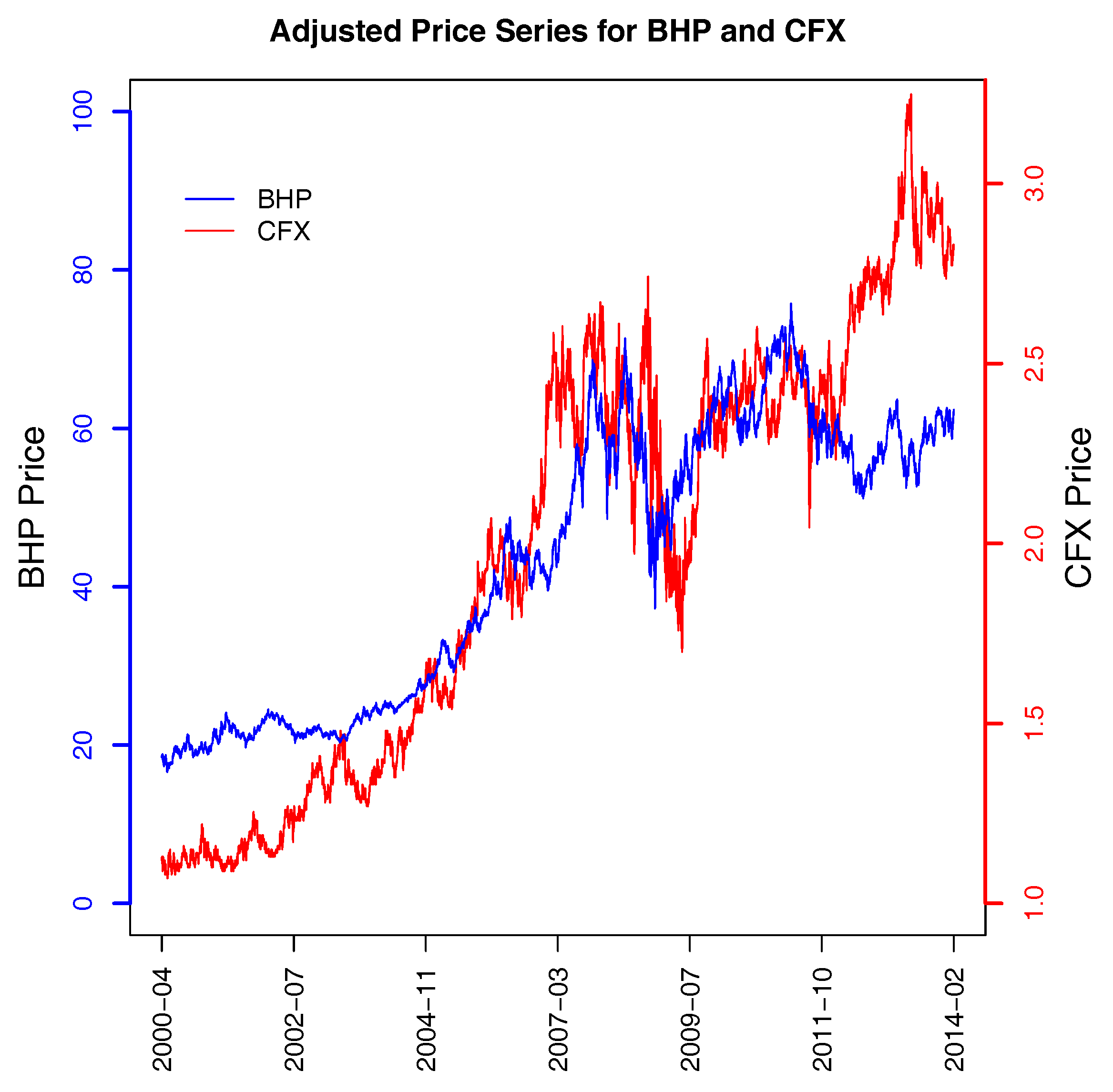
Curiously, the first pair of stocks are not in the same industry. BHP is in Basic Materials and CFX in the real estate industry. They tended to move in the same direction from the start of the study period until 2011. Their price trajectories then began to move in different directions after this time, as can be seen in Figure 4.
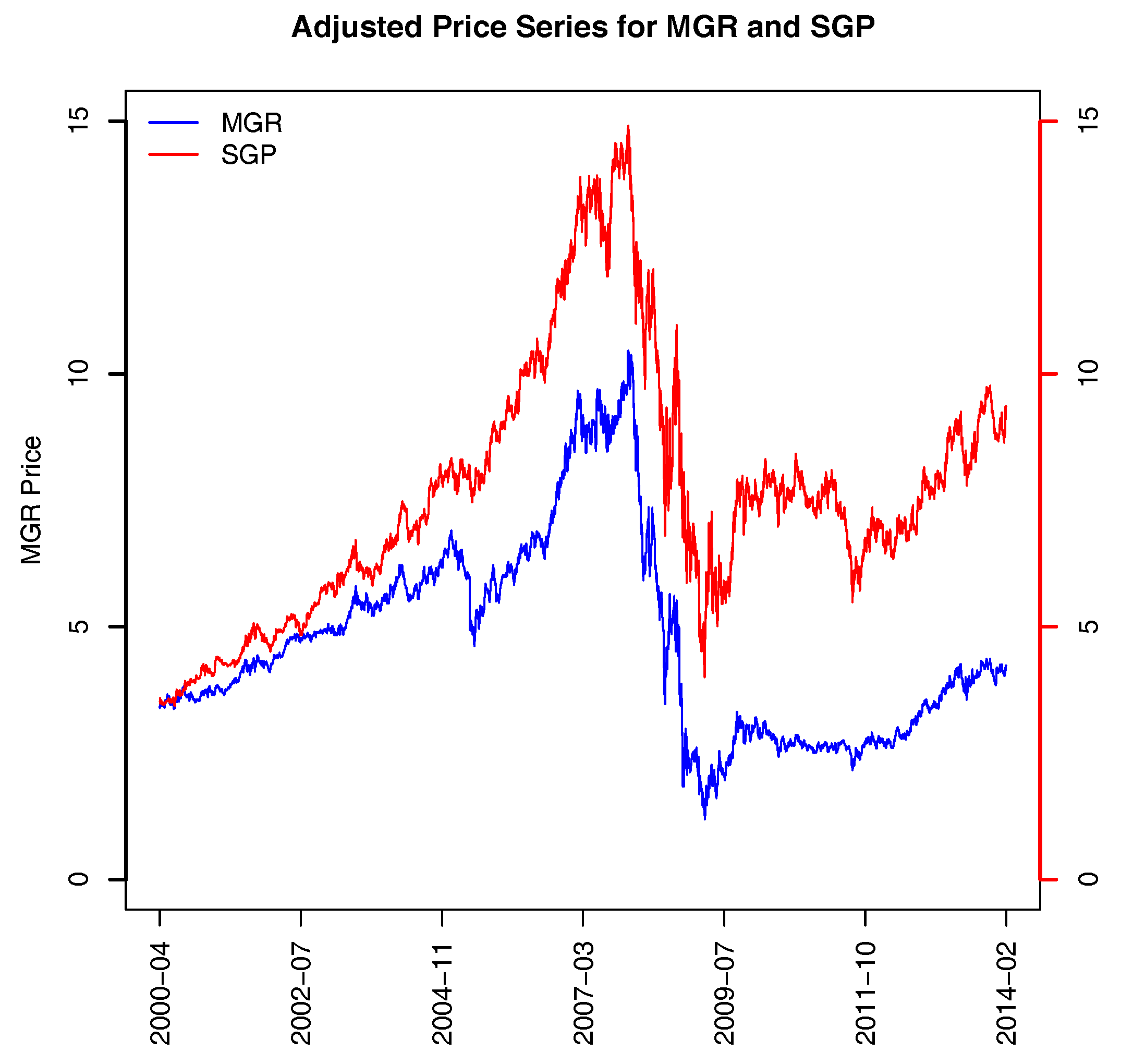
The second pair—MGR and SGP—are both large diversified real estate groups. They had nearly the same stock price level in the beginning of 2000, and have diverged since then. The similarity in their price movements can be easily seen over short time frames, but over the longer term, their price level has diverged, as can be seen in Figure 5.
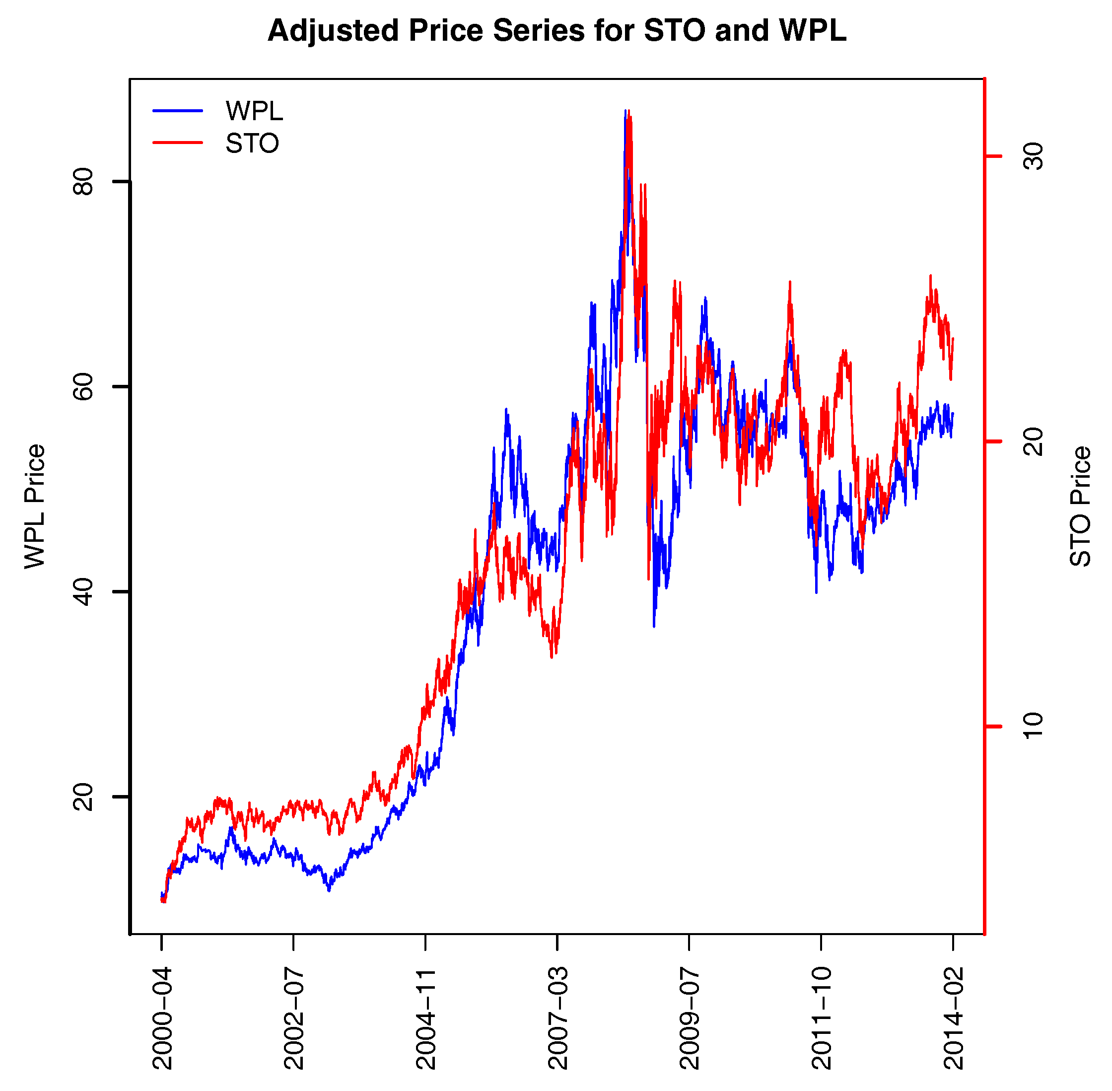
The third pair of stocks are STO and WPL, which are in the Oil & Gas industry. Both companies explore for and produce oil and gas from onshore and offshore wells. The high correlations in their price movements over both the short- and long-term are clearly evident, as can be seen in Figure 6.
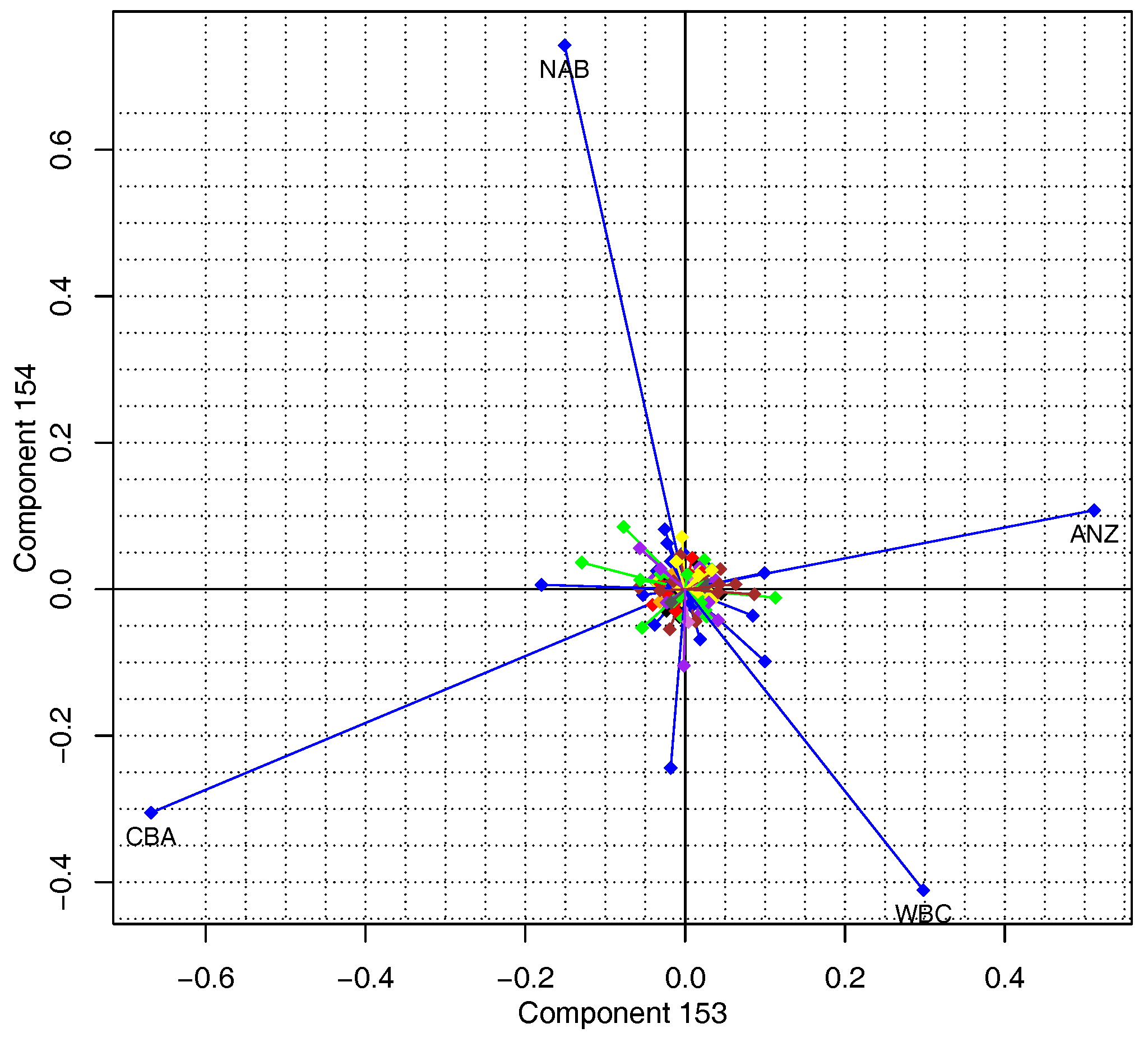
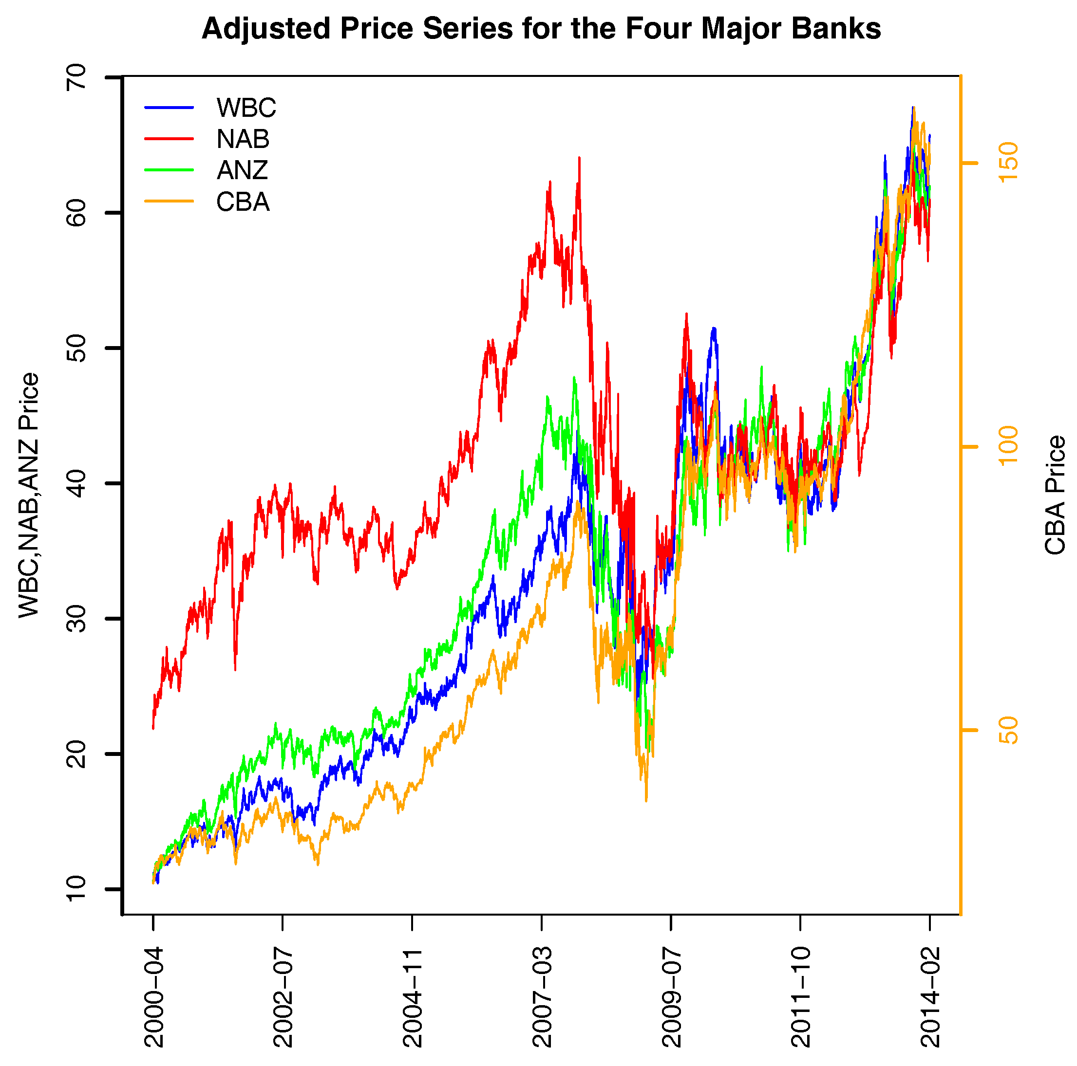
The last four components (PC 153–156, Figure 2 and Figure 3) all picked up the four largest banks in Australia, often referred to as the “four pillars”; their ticker symbols are ANZ, CBA, NAB, and WBC. The strong relationships in price (and consequently returns) are easily seen in Figure 7; their correlations are reported in Table 3. To help in visualizing the price co-movement of the four largest banks, we used a different scale for CBA. Its dividend-adjusted price changed from $20 in the beginning of our study period to approximately $150 at the end of study period, while the other three banks had price levels that ranged from $10 to $70. Obviously, NAB was least correlated with others among the four banks. However, after the 2008 financial crisis, all four banks converged to move very similarly.
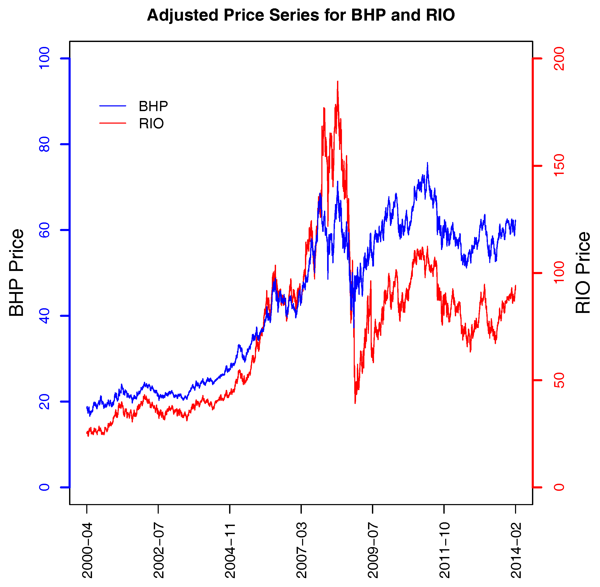
In the scatter plot of PC155 and PC156 (Figure 3), Australia’s two biggest mining firms were also picked up, BHP and Rio Tinto Ltd (RIO). They have a correlation of 0.77 over the sample period (see Table 2). However, they are clearly different from the four banks because they have high loadings of opposite signs in PC155 and near-zero loadings in PC156. A plot of their price trajectories is presented in Figure 8.
In Figure 3 we have the best illustration of Equation (6), because in PC155, BHP and RIO both have loadings whose absolute values are greater than 0.6. Combined, they account for somewhat over 72 percent of the variation, and (as discussed in Section 1) because they are highly positively correlated (see Table 2) their loadings have opposite signs, resulting in a component with only a small amount of variation.
At the beginning of our study period, the price of RIO was approximately 1.4 times that of BHP. Before the price collapsed in 2008, both stocks increased significantly; however, RIO increased more than BHP so that at the end of 2007, the price of RIO was about 2.5 times that of BHP. However, during the 2008 financial crisis, RIO also declined more than BHP. At the end of our study period, the price of RIO was about 1.5 times that of BHP, which is almost the same as it was at the beginning of our study period.
4. Conclusions
As indicated above, our argument is that if a financial analyst undertakes a PCA of a stock or other financial markets as part of their analysis, then they should examine the last few PCs, beginning with the final PC, because they may provide financially useful insights. In this sense, our results above differ from that of other authorities such as Kim and Jeong (2005), who reported that only the market component (PC1) and the subsequent group PCs contained useful information about the financial market analysed. Our results illustrate that further financially useful insights may be contained in the last few principal components because these may identify stocks with near-linear correlations. In the data we examined, the final six components were of this type. The potential existence of such components seems to have been overlooked in the finance literature, despite it being well known in the statistics and econometrics literatures.
The identification of highly correlated stocks (or other assets) can aid in the task of portfolio selection and management because it identifies pairs or groups of stocks which provide little benefit for diversification; holding one of the pair or group will provide most of the benefits of diversification while freeing funds to be invested in other assets. In the data analysed above, holding all four major banking stocks provides very little diversification to a portfolio because their prices all move in a nearly identical manner. It is not a given that such associations exist in any particular market. However, if they do exist, they can be easily detected and that information can be fed into the fund manager’s or other investor’s task of managing their portfolio well.
Even if, for example, a pair of highly correlated stocks are identified, there may be considerations other than diversification which mean that an investor may hold both. Figure 4, Figure 5, and Figure 7 show that high correlations in price movements do not necessarily indicate that the returns over the longer term will be similar. Thus, depending on how much short-fall risk an investor is willing to take on, he or she may decide to hold more than one of the stocks identified in each of these groups.
In our analysis of the Australian Stock Market, we did not find any PCs which indicated the existence of outlier stocks in that market. However, it is possible that other markets may contain such stocks, so a market analyst should examine the PCs to see if evidence of such outliers can be found.
We applied the PCA to the full sample period to illustrate the value of the method. In practical applications, a fund manager would apply the PCA on a rolling window basis to a much shorter period of data. However, our results show that highly correlated stocks tend to remain highly correlated over long periods of time. Nevertheless, these correlations may break down, as is evident in Figure 4. It is clear that the strong correlation between them evident in the first 11 years of the sample ceased to hold in about 2011.
While the method presented here was applied to a stock market, it is general and can be applied to any set of assets for which a correlation matrix can be generated.
Author Contributions
This paper is drawn from Libin Yang’s Master of Commerce thesis entitled “An Application of Principal Component Analysis to Stock Portfolio Management”. William Rea and Alethea Rea were, respectively, the senior and associate supervisors of the thesis. They jointly wrote the paper based on Libin’s work.
Conflicts of Interest
The authors declare no conflict of interest.
Abbreviations
| ANZ | ANZ Bank |
| ASX 200 | Australian Stock Exchange 200 Index |
| BHP | BHP Billiton |
| CBA | Commonwealth Bank |
| CFX | CFS Retail Property Group |
| MGR | Mirva Group |
| NAB | National Australia Bank |
| NVN | Novion Property Group |
| NYSE | New York Stock Exchange |
| PCA | Principal Component Analysis |
| PC | Principal Component |
| RIO | Rio Tinto Ltd |
| SGP | Stockland |
| STO | Santos Limited |
| WBS | Westpac Banking Corporation |
| WPL | Woodside Petroleum Limited |
References
- Aggarwal, Charu C. 2013. Outlier Analysis. New York: Springer. [Google Scholar]
- Barnett, Vic, and Toby Lewis. 1994. Outliers in Statistical Data, 3rd ed. New York: Wiley. [Google Scholar]
- Billio, Monica, Mila Getmansky, Andrew W. Lo, and Loriana Pelizzon. 2012. Econometric measures of connectedness and systemic risk in the finance and insurance sectors. Journal of Financial Economics 104: 535–59. [Google Scholar] [CrossRef]
- Ding, Chris, and Xiaofeng He. 2004. K-means Clustering via Principal Component Analysis. In Paper presented at ICML ’04 Proceedings of the Twenty-First International Conference on Machine Learning, Banff, AB, Canada, 4–8 July; p. 29. [Google Scholar]
- Driessen, Joost, Bertrand Melenberg, and Theo Nijman. 2003. Common factors in international bond returns. Journal of International Money and Finance 22: 629–56. [Google Scholar] [CrossRef]
- Hawkins, Douglas M. 1980. Identification of Outliers. Dordrecht: Springer. [Google Scholar]
- Jolliffe, Ian T. 1986. Principal Component Analysis. New York: Springer. [Google Scholar]
- Kim, Dong-Hee, and Hawoong Jeong. 2005. Systematic analysis of group identification in stocks markets. Physical Review E 72: 046133. [Google Scholar] [CrossRef] [PubMed]
- Kritzman, Mark, Yuanzhen Li, Sebastien Page, and Roberto Rigobon. 2011. Principal Components as a measure of systemic risk. Journal of Portfolio Management 37: 112–26. [Google Scholar] [CrossRef]
- Pérignon, Christophe, Daniel R. Smith, and Christophe Villa. 2007. Why common factors in international bond returns are not so common. Journal of International Money and Finance 26: 284–304. [Google Scholar]
- R Core Team. 2014. R: A Language and Environment for Statistical Computing. Vienna: R Foundation for Statistical Computing. [Google Scholar]
- Yang, Libin, William Rea, and Alethea Rea. 2016. Stock Selection with Principal Component Analysis. Journal of Investment Stategies 5: 1–21. [Google Scholar]
- Zheng, Zeyu, Boris Podobnik, Ling Feng, and Baowen Li. 2012. Changes in cross-correlations as an indicator for systemic risk. Scientific Reports 2: 888. [Google Scholar] [CrossRef] [PubMed]
Figure 1.
Scatter plots of relative weights of each stock in components 151 and 152 arising from a principal components analysis (PCA) on a correlation matrix from the whole study period. The lines join the origin to the point representing the coefficient in the 151th eigenvalue (x-axis) and 152nd eigenvalue (y-axis). The stocks are colour-coded using the Industry Classification Benchmark Industry (ICB) classification. Financials are blue (33 stocks), Health Care are red (9 stocks), Industrials are yellow (24 stocks), Consumer Services are brown (19 stocks), Basic Materials are green (31 stocks), Oil & Gas are purple (16 stocks), Utilities are orange (5 stocks), Consumer Goods are black (9 stocks), Telecommunications are orchid (4 stocks), Technology are grey (6 stocks). Stocks with a loading of at least 0.2 in one of the PCs are labelled with their ticker symbol. From this scatterplot, we can conclude that there are six highly correlated stocks structured as three pairs: namely, STO and WPL, SGP and MGR, and BHP and CFX.
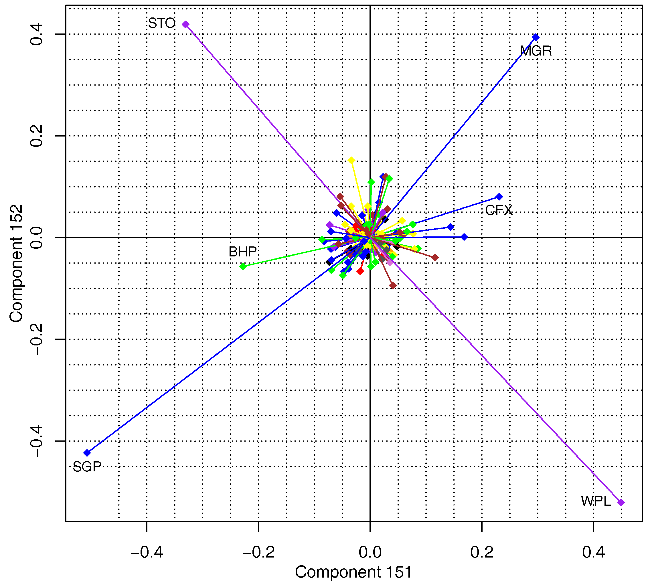
Figure 2.
Scatter plots of relative weights of each stock in components 153 and 154 arising from a PCA on a correlation matrix from the whole study period. The lines join the origin to the point representing the coefficient in the 153rd eigenvalue (x-axis) and 154th eigenvalue (y-axis). The stocks are colour-coded using the colour scheme described in Figure 1. Stocks with a loading of at least 0.25 in one of the PCs are labelled with their ticker symbol. From this scatterplot, we can conclude that there are four highly correlated stocks structured as two pairs: namely, CBA (Commonwealth Bank of Australia) and ANZ (ANZ), and NAB (National Australia Bank) and WPC (Westpac).

Figure 3.
Scatter plots of relative weights of each stock in components 155 and 156 arising from a PCA on a correlation matrix from the whole study period. The lines join the origin to the point representing the coefficient in the 155th eigenvalue (x-axis) and 156th eigenvalue (y-axis). The stocks are colour-coded using the colour scheme described in Figure 1. Stocks with a loading of at least 0.2 in one of the PCs are labelled with their ticker symbol. From this scatterplot, we can conclude that there are six highly correlated stocks structured as three pairs: namely, CBA and WBC, NAB and ANZ, and BHP and RIO.
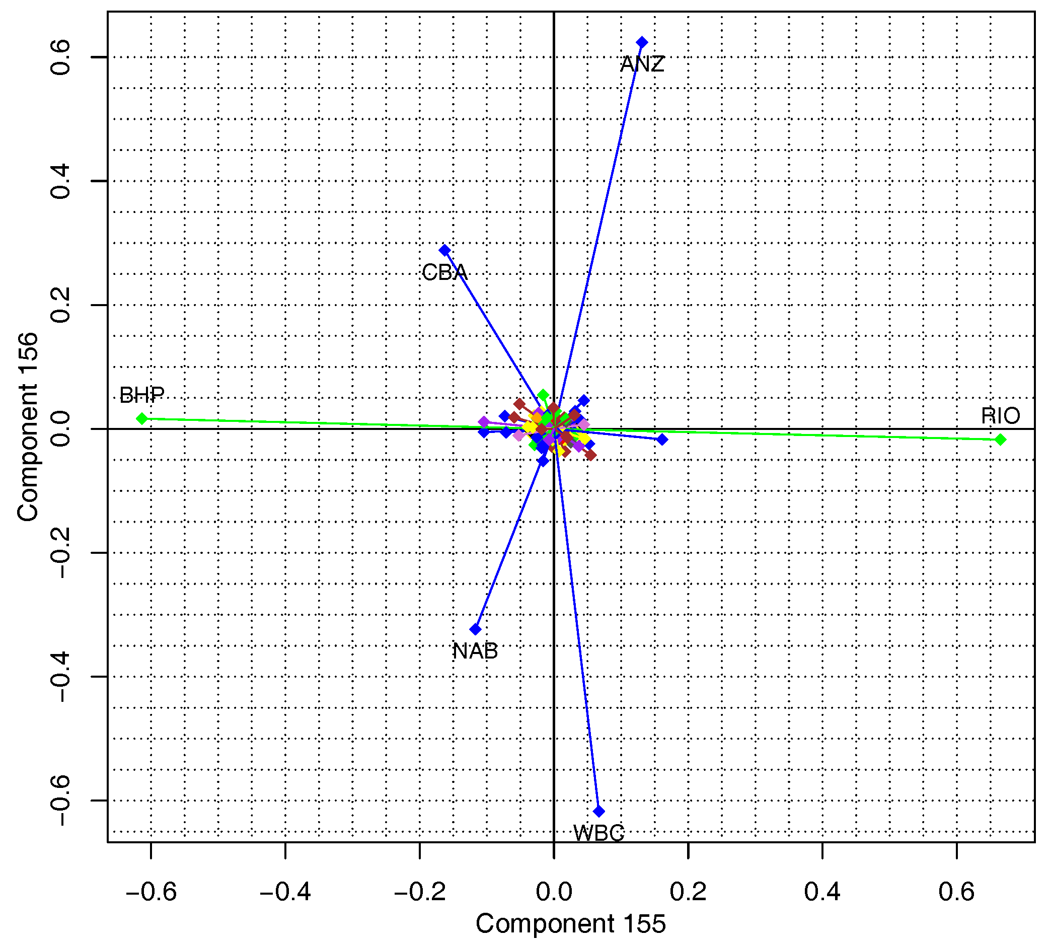
Figure 4.
Time series plot of two stocks identified in the scatter plot of components 151 and 152: BHP-Billiton (BHP) in basic materials and CFS Retail Property Trust Group (CFX) in the real estate industry.
Figure 4.
Time series plot of two stocks identified in the scatter plot of components 151 and 152: BHP-Billiton (BHP) in basic materials and CFS Retail Property Trust Group (CFX) in the real estate industry.

Figure 5.
Time series plots of near-linear correlated stocks identified in a scatter plot of components 151 and 152: Mirvac Group (MGR) and Stockland Corporation Limited (SGP)—two stocks in the real estate sector.
Figure 5.
Time series plots of near-linear correlated stocks identified in a scatter plot of components 151 and 152: Mirvac Group (MGR) and Stockland Corporation Limited (SGP)—two stocks in the real estate sector.

Figure 6.
Time series plot of two stocks in the Oil & Gas industry identified in the scatter plot of components 151 and 152: Santos (STO) and Woodside Petroleum (WPL).
Figure 6.
Time series plot of two stocks in the Oil & Gas industry identified in the scatter plot of components 151 and 152: Santos (STO) and Woodside Petroleum (WPL).

Figure 7.
Time series plots of near-linear correlated stocks identified in the scatter plots of components 153 to 156: the four big banks in Australia. ANZ (ANZ), Commonwealth Bank of Australia (CBA), National Australia Bank (NAB) and Westpac (WBC).
Figure 7.
Time series plots of near-linear correlated stocks identified in the scatter plots of components 153 to 156: the four big banks in Australia. ANZ (ANZ), Commonwealth Bank of Australia (CBA), National Australia Bank (NAB) and Westpac (WBC).

Figure 8.
Time series plot of two stocks in Basic Materials identified in component 155: BHP and Rio Tinto (RIO).
Figure 8.
Time series plot of two stocks in Basic Materials identified in component 155: BHP and Rio Tinto (RIO).


Table 1.
Eigenvalues and variances explained by the last six principal components. The percent of variation explained was calculated using Equation (1).
Table 1.
Eigenvalues and variances explained by the last six principal components. The percent of variation explained was calculated using Equation (1).
| Eigenvalue | Variance Explained (%) | |
|---|---|---|
| PC151 | 0.398 | 0.255% |
| PC152 | 0.380 | 0.244% |
| PC153 | 0.321 | 0.206% |
| PC154 | 0.304 | 0.195% |
| PC155 | 0.286 | 0.183% |
| PC156 | 0.244 | 0.157% |
Table 2.
The correlations of stocks with near-linear relationships in principal components (PCs) 151, 152, and 155. See Figure 1 and Figure 3.
| Pair | Correlation | PCs |
|---|---|---|
| MGR-SGP | 0.71 | 151, 152 |
| STO-WLP | 0.95 | 151, 152 |
| BHP-RIO | 0.77 | 155 |
Table 3.
Price correlation coefficients of the four largest banks.
| ANZ | WBC | CBA | NAB | |
|---|---|---|---|---|
| ANZ | 1 | 0.97 | 0.96 | 0.85 |
| WBC | 0.97 | 1 | 0.98 | 0.76 |
| CBA | 0.96 | 0.98 | 1 | 0.73 |
| NAB | 0.85 | 0.76 | 0.73 | 1 |
© 2017 by the authors. Licensee MDPI, Basel, Switzerland. This article is an open access article distributed under the terms and conditions of the Creative Commons Attribution (CC BY) license (http://creativecommons.org/licenses/by/4.0/).
Share and Cite
MDPI and ACS Style
Yang, L.; Rea, W.; Rea, A. Financial Insights from the Last Few Components of a Stock Market PCA. Int. J. Financial Stud. 2017, 5, 15. https://doi.org/10.3390/ijfs5030015
AMA Style
Yang L, Rea W, Rea A. Financial Insights from the Last Few Components of a Stock Market PCA. International Journal of Financial Studies. 2017; 5(3):15. https://doi.org/10.3390/ijfs5030015
Chicago/Turabian StyleYang, Libin, William Rea, and Alethea Rea. 2017. "Financial Insights from the Last Few Components of a Stock Market PCA" International Journal of Financial Studies 5, no. 3: 15. https://doi.org/10.3390/ijfs5030015
Note that from the first issue of 2016, this journal uses article numbers instead of page numbers. See further details here.