
Does Gold Act as a Hedge and a Safe Haven for China’s Stock Market?


School of Finance and Statistics, Hunan University, Changsha, Hunan 410079, China
*
Author to whom correspondence should be addressed.
Int. J. Financial Stud. 2017, 5(3), 18; https://doi.org/10.3390/ijfs5030018
Submission received: 28 June 2017
/
Revised: 5 August 2017
/
Accepted: 8 August 2017
/
Published: 17 August 2017
Abstract
:This paper examines the dynamic relationships between gold and stock markets in China. Using daily gold and stock indexes data, we estimated the DCC-GARCH model for the five bear markets since 31 October 2002, and simultaneously used different segments of China’s stock markets for analysis. Our main objective was to examine the time-varying correlations between gold and stock and to check the effectiveness of gold as a hedge or a safe haven for stocks. Results showed that: (1) the dynamic conditional correlations switched between positive and negative values over the periods under study; (2) due to the increasing investment demand of gold, the hedging effect of gold on China’s stock market has strengthened remarkably. Gold acts as a safe haven for only the latest two of the five bear markets analyzed (12 June 2015–26 August 2015 and 22 December 2015–29 February 2016); and (3) for non-bear markets, gold does not offer good risk hedging.
1. Introduction
Gold is one of the most malleable, ductile, dense, conductive, non-destructive, brilliant, and beautiful of metals. This unique set of qualities has made it a coveted object throughout history by humans in almost every civilization, and there have been active gold markets for over 6000 years (Green 2007). As money, as an investment, as a store of value, gold has long fascinated the financial media, investors and researchers in equal measure. Since the breakdown of the Bretton Woods System, gold is no longer a central cornerstone of the international monetary system, but nevertheless still attracts considerable attention from investors and researchers. Owing to the increasing uncertainty of the global financial markets, diversifying a portfolio through hedging becomes more important (Beckmann et al. 2015) especially, since during the global financial and economic crisis that started in 2007, financial assets (in particular stock prices) exhibited losses while the gold price experienced an intense increase. Figure 1 shows the evolution of the Shanghai Stock Exchange (SSE) Composite Index and the price of gold from 31 October 2016. Since the beginning of the financial crisis in October 2007, the SSE Composite Index has fallen 38%, while the gold price has risen 22%1. The performance of gold is most impressive given the losses suffered in other asset classes during the crisis. The paper aimed to investigate the dynamic relationships between gold and stocks and to test whether gold represents a safe heaven or as a hedge against China’s stock market.
Among all financial assets, gold is quite unique and virtually sits as its own asset class that differs from other precious metals including silver, platinum, and palladium (Batten et al. 2010, 2014). One reason is that its usefulness as an industrial metal is small and declining when compared with its investment and uses in jewelry. The other precious metals still have significant uses in industry: platinum is commonly used in catalysts, palladium is now mixed into many of the alloys that are replacing gold in dentistry and silver can be used in the production of solar panels (O’Connor et al. 2015). According to the 2016 Chinese Gold Yearbook published by the China Gold Association, physical gold transactions in the Shanghai gold exchange have been the highest in the world for nine consecutive years. Figure 2 shows the gold production and consumption by China from 2009–2016. Gold production increased annually and reached 453,486 tons in 2016. China has been the world’s largest gold producer for 10 consecutive years. The gold consumption of China reached 975.38 tons in 2016, and China has been the world’s top gold consumer for four consecutive years; however, gold consumption in 2016 declined by 6.74% when compared to 2015. From 2015 to 2016, the use of gold in jewelry in China decreased by 18.91%, while the use of gold bars increased by 28.19% and the use of gold coins increased by 10.14%. Although the consumption of gold has sharply declined, gold as an investment in China has increased dramatically, with a total growth of almost 30%. Gold has a dual nature of commodity and finance, so the demand for gold is generally divided into two parts: the consumption demand and the investment demand. With the development of China’s gold market, there is a growing variety of gold investment demands as well as gold investment products. As the world’s largest gold consumer and producer, checking whether gold is a safe haven or hedge for China’s stock market is of great significance for Chinese investors, as well as investment product designers. While the research related to this field are rather scarce, one existing study on the hedging potential of gold traded on the relatively new Shanghai Gold Exchange was that of Hoang et al. (2015). They investigated the role of gold quoted on the Shanghai Gold Exchange in the diversification of Chinese portfolios from 2004–2014. Against this background, this paper estimated the DCC-GARCH model for daily gold and stock data for the five bear markets in China, examined the dynamic relationships between the gold and stock markets, and checked the effectiveness of gold as a hedge or a safe haven for stock markets.
2. Related Literature
Investors and financial analysts often emphasize that gold acts as an alternative investment asset to counter market risk in times of market stress; not surprisingly, the hedge and safe heaven potentials of gold have been extensively analyzed in market fluctuations. Baur and Lucey (2010) were the first to formulate empirically testable definitions for a hedge and a safe haven with regard to financial assets such as stocks. Following their definitions, a hedge (safe haven) is an asset that is uncorrelated (negatively correlated) with another asset or portfolio on average (only in times of market stress or turmoil) (Beckmann et al. 2015) and reported that gold was a safe haven for stocks in the US, the UK and Germany. Gold was also found as a hedge for stocks in the US and the UK. Their analysis revealed that gold was not a safe haven for stocks at all times, but only in extreme bearish stock markets and that the safe haven property was short-lived. Baur and Mcdermott (2010) also distinguished between a strong and a weak form of the hedge and the safe haven property (Beckmann et al. 2015). Gürgün and Ünalmıs (2014); Beckmann et al. (2015); Nguyen et al. (2016); Iqbal (2017) and Shahzad et al. (2017) all found that gold could act as a hedge and safe haven in emerging and developing countries, European stock markets, five Eurozone peripheral GIPSI countries, and Pakistan and India, respectively. For countries with a religion factor such as Malaysia and the GCC (Gulf Cooperation Council: Bahrain, Kuwait, Oman, Qatar, Saudi Arabia and United Arab Emirates), the domestic Islamic gold account provided hedge and safe haven to sharia compliant stocks (Ghazali et al. 2015; Mensi et al. 2015, 2016). Ciner et al. (2013); Chen and Lin (2014); Choudhry et al. (2015) and Smiech and Papiez (2016) also depicted that gold had characteristics of a hedge and safe haven for the US stock market. According to the analysis above-mentioned, most of the previous research has shown that gold can act as a safe haven against extreme market movement and as a hedge on average.
Other studies have examined the dynamic relationship between gold and stock. Souček (2013) found that during unstable periods, the correlation between gold and stock, proxied by open interest, tended to be weak or negative. Thus, gold can serve as an investors’ safe haven. Baruník et al. (2016) investigated the dynamic correlations between gold and stocks. Their analyses showed that heterogeneity in correlations across a number of investment horizons between gold and stock was a dominant feature during times of economic downturn and financial turbulence. Heterogeneity prevailed in correlations between gold and stocks. After the 2008 crisis, correlations among gold and stock increased and became homogenous.
A number of studies have focused on the relationship between gold and stock in emerging economies. For example, Jain and Biswal (2016) investigated the dynamic linkages between the prices of gold and Indian stocks and uncovered a strong relationship between gold and stocks, suggesting the importance of using gold to restrain stock market volatility. However, the study by Basher and Sadorsky (2016) was based on data from 23 emerging economies, which indicated that there was a positive link between gold and stocks in most emerging economies. Bouri et al. (2017) also found that there was a positive nonlinear relationship between gold and the stock market in India. Dee et al. (2013); Arouri et al. (2015) and Huang et al. (2016) all focused their studies on the relationship between gold and stocks in China.
From the existing literature, we uncovered several things. For the method, most of the studies used the quantile-GARCH model, and some of them used the DCC-GARCH model, Copula and wavelet analysis. For the results, gold was negatively related to stocks in most countries, so gold could be used as a hedge and a safe haven asset. The main feature of these studies, which partially motivated our research, was to first use a quantile regression approach which included a simple GARCH (1,1) model; Baur and Lucey (2010) analyzed gold’s safe-haven role in the stock market, however, their analyses were based on the short-term extreme negative impact of stocks on days, which adapted to the characteristics of the “slow bull and quick bear” in western stock markets. For the characteristics of a “quick bull and slow bear” in China’s stock markets, bear markets are usually measured in months or years. Dividing the time period into bear market periods and nonbear market periods based on the fluctuating situation in China’s stock market was more realistic to study whether gold could play the role of a safe haven and hedge in different periods. Second, the previous literature has only used the SSE Composite Index as the proxy variable for China’s stock market, therefore, this paper selected the SSE Composite Index, the SZSE Component Index, the CSI 300 Index, the SME Index, and GEM Index simultaneously to research the effectiveness of gold as a hedge or a safe haven for different stock indexes during the bear and nonbear markets. The results could describe the overall relationship between gold and China’s stock market.
3. Data, Definitions, Empirical Methodology
3.1. Data
As indicated above, the five stock indexes used were the Shanghai Stock Exchange Composite Index (SSE)2, the Shenzhen Stock Exchange Component Index (SZSE)3, the Capitalization-weighted Stock Index 300 Index (CSI)4, the Small and Medium Enterprise Board Index (SME)5 and the Growth Enterprise Market Index (GEM)6. The paper used the AU9995 spot price from the Shanghai Gold Exchange (SGE) as the proxy variable for China’s gold price. The start date of AU9995 was 31 October 2002, so the sample period spanned 31 October 2002 to 18 April 2017. However, the start date of the CSI 300 Index, the SME Index and the GEM Index were April 2005, June 2005 and June 2010, respectively. Thus, the starting times of the above-mentioned three kinds of index were different from the SSE Composite Index and the SZSE Component Index, as shown in Table 1. Daily data of the five stock indexes and gold spot prices were obtained from Datastream and SGE. The continuous returns for both stock and gold prices were calculated by taking the natural logarithm of the ratio of two consecutive prices, which was then, multiplied it by 100.
Table 2 presents the descriptive statistics for the daily return series of the gold and five stock indexes and unit root tests for returns. As shown in panel A, all stock index returns varied more dramatically than the gold returns as indicated by their simple standard deviation. Skewness coefficients showed that the return distribution for all time series were negatively and significantly skewed. Kurtosis coefficients indicated that all return series were far from normally distributed. In addition, the Jarque–Bera test statistics clearly confirmed the rejection of the null hypothesis of normality for all returns series at the 1% significance level for both the stock indexes and gold series.
Panel B presents the results of the four unit root and stationarity tests namely the DF, ADF, DF-GLS and PP tests. The DF, ADF, and PP test statistics were significant at the 1% significance level, rejecting the null hypothesis of unit root for all time return series. Referring to the DF-GLS results, we could not reject the null hypothesis of stationarity only for the SME Index. Consequently, all the return series were stationary and thus suitable for further analysis.
Financial time series often exhibit correlation. Under such conditions, GARCH modeling is particularly appropriate. Table 3 shows the results of the Ljung-Box test and ARCH test. The Ljung-Box test indicated evidence of autocorrelation in the return series for both the gold and stock indexes. Furthermore, the empirical statistics of the Engle (1982) test for conditional heteroscedasticity were significant for all cases suggesting the presence of ARCH effects in returns. All these features justified our choice of GARCH type models to examine the dynamic relationship between gold and stock indexes.
3.2. Definitions of Bear and Nonbear Stock Markets in China
At present, there are two main methods to divide the cycle of the bull market and the bear market: (i) the parameter method where Hamilton (1989) divided the bear market and bull market by estimating the parameters of the Markov-switching model; and (ii) the nonparametric method, which divides the bull and bear markets by looking for peaks and troughs. The parameter method is more suitable for mature markets such as the US and Europe. Considering the particularity of the Chinese capital market, which is immature and vulnerable to national policy, the nonparametric method was adopted in this paper to divide bull and bear markets in China. Referring to Eliot wave theory (Frost and Prechter 2005) and combining the characteristics of policy intervention and institutional change in China’s stock market development (Lu and Xu 2004), this paper found that the SSE composite index contained five bear markets from 31 October 2002 to 18 April 20177, as shown in Table 4 and Figure 3. In addition to the five bear markets, other periods including bull markets and shock markets were considered as normal or nonbear markets. The “bear market periods” and the “nonbear market periods” of the other four stock indexes were all consistent with the SSE Composite Index.
3.3. Methodology
Following the definitions of Baur and Lucey (2010), a hedge (safe haven) is an asset that is uncorrelated or negatively correlated with another asset or portfolio on average (in times of market stress or turmoil). We estimated the dynamic conditional correlations between the return of gold and five stock indexes in times of bear market periods and nonbear market periods. That is, if gold was uncorrelated or negatively correlated with stocks in times of bear market periods (or nonbear market periods), gold can be a safe haven (hedge) for stock markets.
The aim of this paper is to investigate contemporaneous time-varying correlation between gold and stock index in different periods, the correlations thus obtained will shed light on the dynamic relationships amongst the variables. The DCC-GARCH model by Engle (2002) is used to examine time varying correlations between two or more series. So, using the DCC-GARCH framework is more appropriate than other GARCH models. The DCC-GARCH model is estimated in two steps: in the first step, the GARCH parameters are estimated; and in the second step, the conditional correlations are estimated.
Ht is a n × n conditional covariance matrix, Rt is the conditional correlation matrix, and Dt is a diagonal matrix with time-varying standard deviations on the diagonal.
The expressions for h are univariate GARCH models (H is a diagonal matrix). For the GARCH (1,1) model, the elements of Ht can be written as:
where Qt is a symmetric positive definite matrix.
where is the n × n unconditional correlation matrix of the standardized residuals . The parameters and are non-negative, and are associated with the exponential smoothing process used to construct the dynamic conditional correlations. The DCC model is mean reverting as long as + < 1. Dependence on only parameters and is one of the strengths of this model. Irrespective of the number of variables, only these two parameters need to be estimated, making it more likely to reach an optimal solution.
When the standardized residuals from two variables rise or fall together, they push the correlation up. This elevated level will gradually decrease back to the average level over the passage of time due to the complete absorption of information. When the residuals move in different directions, they pull the correlation down, which moves up with time. The speed of this process is controlled by the parameters and .
The correlation estimator is
For the purposes of this study, the focus of interest is , which represents the conditional correlation between the return of gold and the return of each stock index pair.
4. Empirical Results
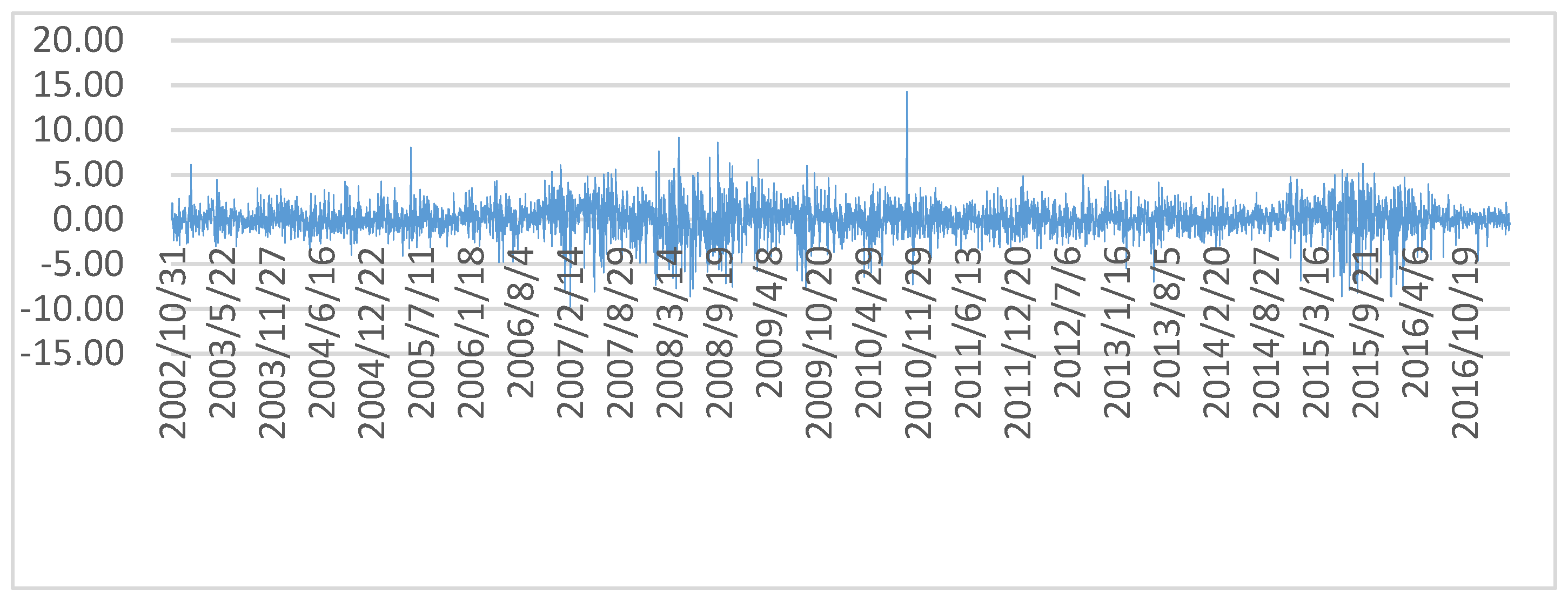
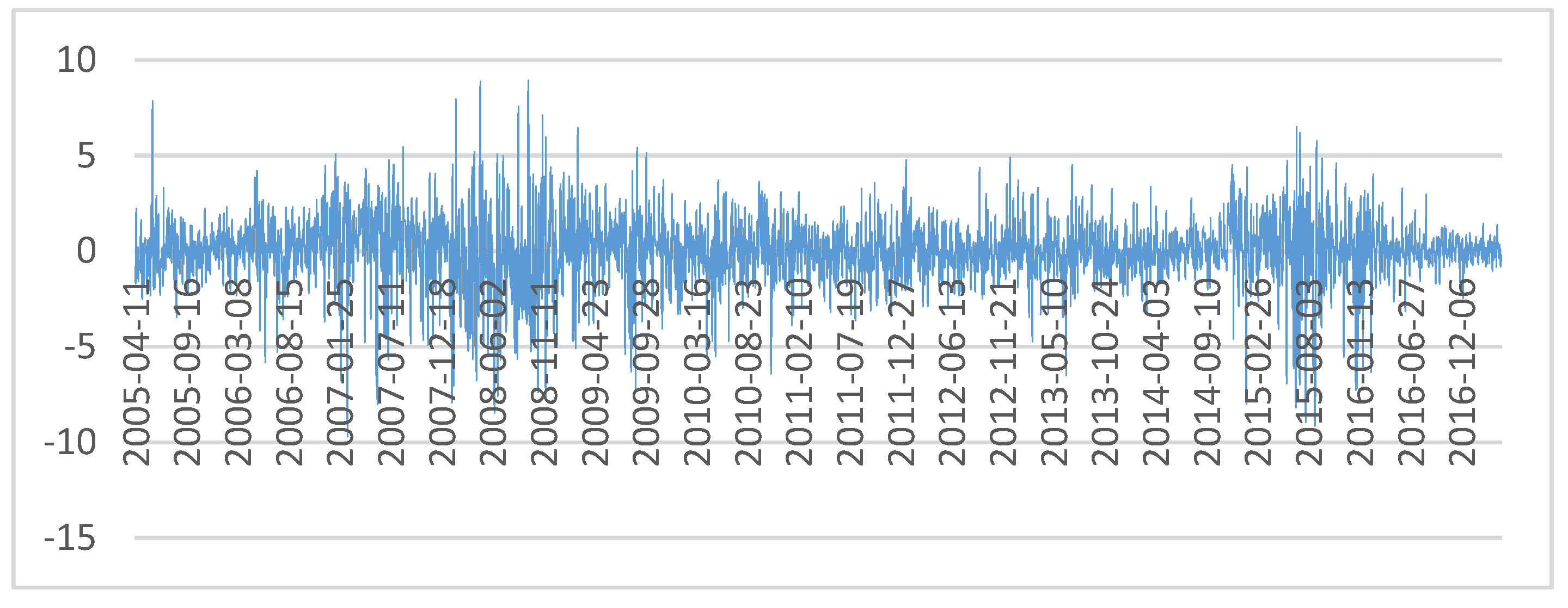
Time series graphs of returns show how volatility has changed across time (Figure 4, Figure 5, Figure 6, Figure 7, Figure 8 and Figure 9). Each series displays several periods of volatility clustering, which also confirms the conclusions from Table 3 that ARCH effects exist in each yield series8. It is reasonable to assume that the GARCH model is appropriate.
First, the time-varying variances of the series were estimated using a univariate GARCH specification, and the parameter estimates are presented in Table 5. α and β represent the estimated ARCH (1) and GARCH (1) parameters, respectively. All univariate GARCH processes showed a high degree of persistence, that is, the sum of α and β were all close to one, indicating that all the models were of good fit. The low values of α and the high values of β indicated that the correlation process was resistant to shocks and reverted to mean quickly. This indicated that the correlations amongst the variables were stable.
The magnitude of the GARCH cofficient (β) for stock indexes were high and varied between 0.914 and 0.945, and the magnitude of the GARCH cofficient (β) for gold as around 0.9, indicating the high persistence of volatility over time.
According to Engle (2002), the DCC (1,1) model is the most suitable for fitting a financial time series. The multivariate GARCH model of dynamic conditional correlations was estimated using the maximum likelihood estimation. To account for non-normality in the distribution of returns, the DCC-GARCH was estimated with a multivariate student t distribution. The DCC (1,1)–GARCH (1,1) parameter estimates are presented in Table 6.
The estimated DCC parameters, and , implied a persistent correlation. The sum of and was closer to one, so the dynamic correlation was more obvious. Thus, the dynamic correlation between the SSE Composite Index and gold was the strongest, while the dynamic correlation between the CSI 300 index and gold was the weakest.
The magnitude of mean dynamic conditional correlation coefficients varied between −1 and 1. If the coefficient was closer to −1, the negative correlation between gold and stock index was stronger. In contrast, when the coefficient was closer to 1, the positive correlation between gold and stock index was stronger. If the coefficient was equal to 0, gold had no relation with the stock indexes. The mean dynamic conditional correlations between stock indexes and gold are presented in Table 7.
The mean dynamic conditional correlations between SSE-Gold and SZ-Gold were positive in the period of Bear Market I, and both of their values were close to 0.1. This indicates that gold could not act as a safe haven during Bear Market I. The relationship of gold and the CSI 300 Index, the SME Index and the GEM Index could not be analyzed since these three indexes did not exist at this time.
The mean dynamic conditional correlations between SSE-Gold, SZ-Gold, CSI-Gold, and SME-Gold were all positive in the period of Bear Market II. Similarly, the mean dynamic conditional correlations between SSE-Gold, SZ-Gold, CSI-Gold, SME-Gold and GEM-Gold were all positive in Bear Market III. This finding indicated that gold did not act as a safe haven for stock indexes in Bear Markets II and III.
With the exception that the mean dynamic conditional correlation coefficient of CSI-Gold was greater than 0, the mean dynamic conditional correlation coefficients of SSE-Gold, SZ-Gold, SME-Gold and GEM-Gold were all less than 0 in Bear Market IV. These four dynamic conditional correlation coefficients varied between −0.02 and −0.05, indicating that gold was negatively related to most stock indexes, so gold was a safe haven asset for stocks in Bear Market IV. Moreover, the mean dynamic conditional correlation coefficients of SSE-Gold, SZ-Gold, CSI-Gold, SME-Gold and GEM-Gold were all less than 0 in Bear Market V, which varied between 0 and −0.01. This showed that gold could also act as a safe haven in Bear Market V. This can be explained that with the increase in investment demand for gold, more investors tended to include gold in their investment portfolio to diversify risk.
The mean dynamic conditional correlation coefficients of SSE-Gold, SZ-Gold, CSI-Gold, SME-Gold, and GEM-Gold were greater than 0 in the non-bear markets. Among them, the mean dynamic conditional correlation coefficient of CSI-Gold was the largest at 0.0669, and the minimum mean dynamic conditional correlation coefficient was GEM-Gold, which was 0.0344. This showed that not only was gold not used as an investment hedge, but was instead invested just like a stock during periods of non-bear markets.
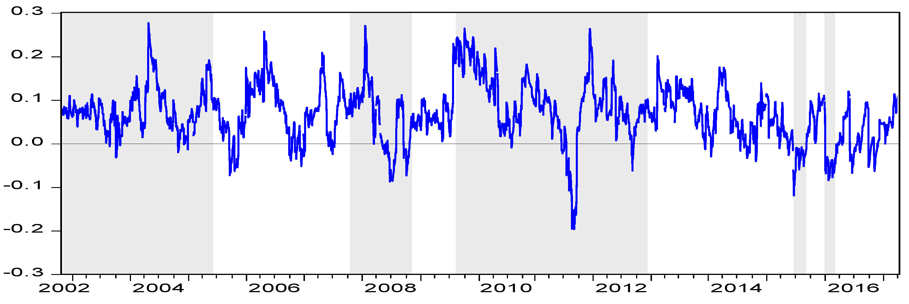
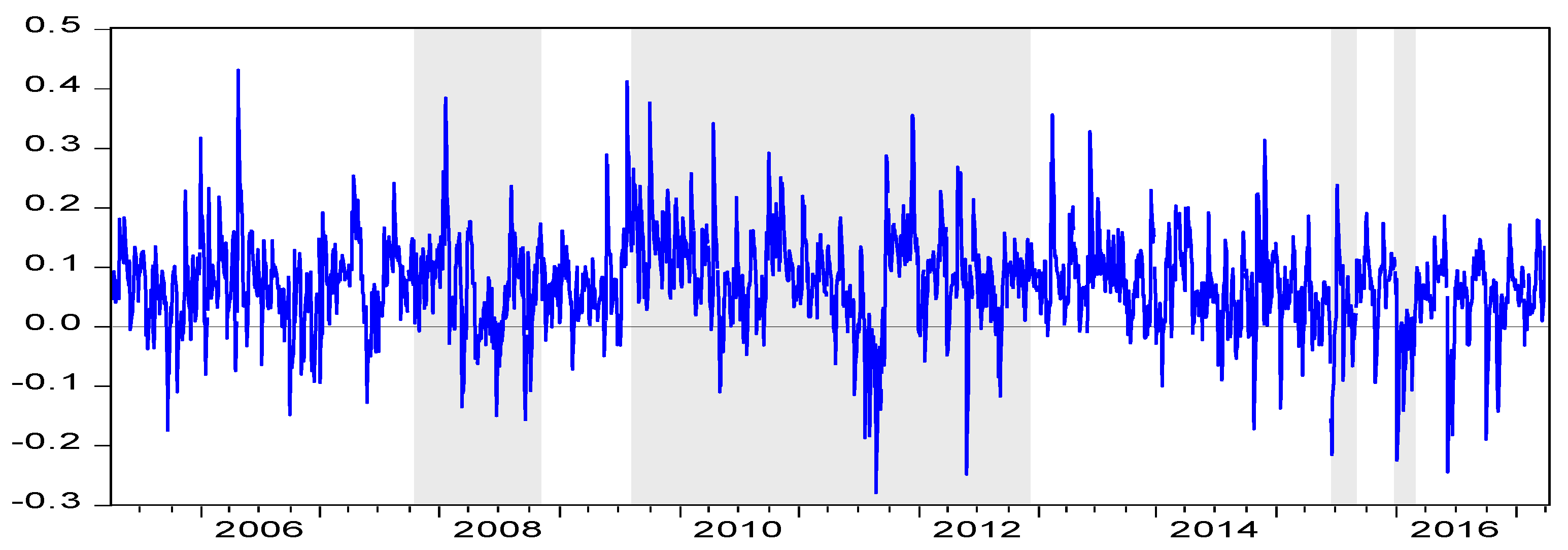
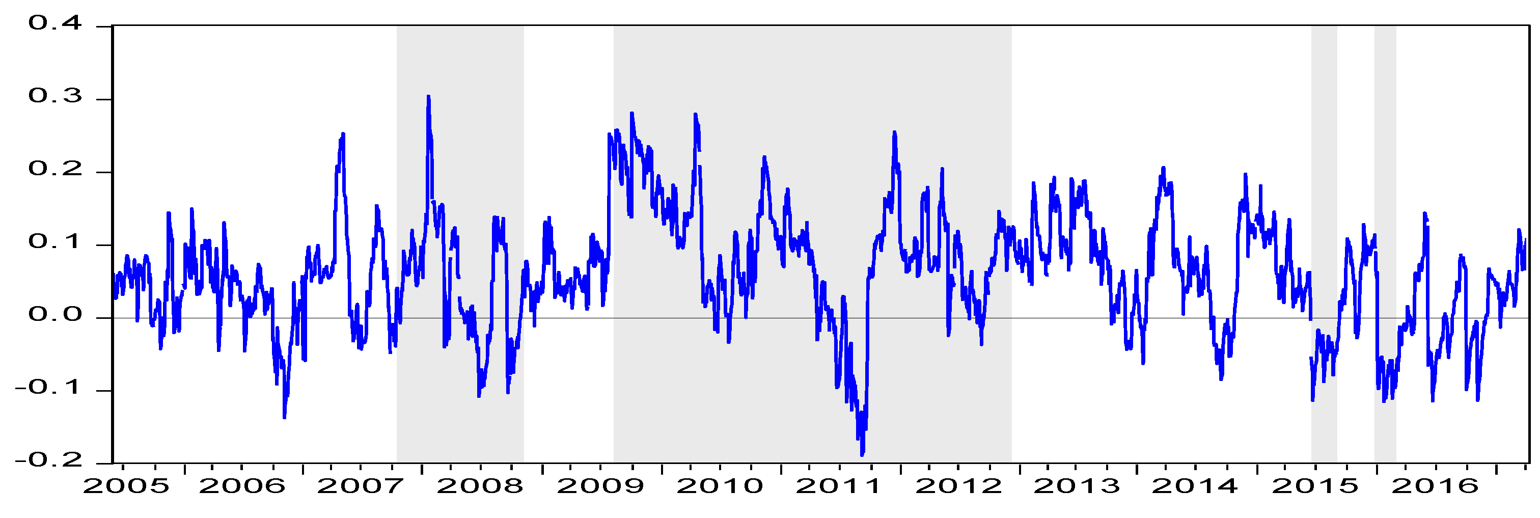
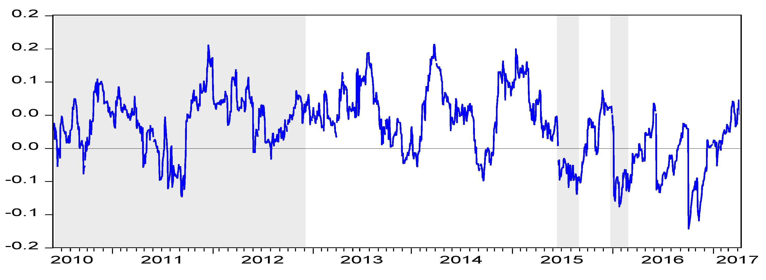
Figure 10, Figure 11, Figure 12, Figure 13 and Figure 14 show the evolution over time of the dynamic conditional correlation coefficient
. The sign of all correlation coefficients was consistently negative over Bear Markets IV and V (12 June 2015–26 August 2015 and 22 December 2015–29 February 2016); that is, there was a negative relationship between gold and the five stock indexes, so gold was a safe haven asset for stocks. However, the correlation coefficients sign was consistently positive in nonbear market periods (see non-shadow section in Figure 8, Figure 9, Figure 10, Figure 11 and Figure 12), where gold did not act as a hedge for stocks in China.
5. Subsample Test
Subsamples of bear and nonbear market periods were also estimated in Table 8, Table 9, Table 10, Table 11 and Table 12. The results were almost consistent with Table 7, where gold acted as a safe haven for only the latest two of the five bear market periods (12 June 2015–26 August 2015 and 22 December 2015–29 February 2016); however, gold did not offer good risk hedging for nonbear market periods. Nevertheless, due to the limited number of observations, many estimates were not stable (see the blue font, and “/” indicates it could not be estimated).
6. Conclusions
Against a background of intensified macroeconomic uncertainty, whether gold can play its traditional role of stored value effectively and become a hedge and safe haven asset for the stock market is a question worth discussing. This paper examined the dynamic relationships between the returns of the Shanghai gold spot price and the returns of the SSE Composite Index, the SZSE Component Index, the CSI 300 Index, the SME Index, and the GEM Index, using daily data from 31 October 2002 to 18 April 2017, which contained five bear markets. Our analysis yielded several noteworthy findings. First, gold was a safe haven for the SSE Composite Index, the SZSE Component Index, the CSI 300 Index, the SME Index, and the GEM Index only in Bear Market V (22 December 2015–29 February 2016); with the exception of the CSI 300 Index, gold as a safe haven for the SSE Composite Index, the SZSE Component Index, the SME Index and the GEM Index in Bear Market IV (12 June 2015–26 August 2015), while in the other three bear markets, gold did not act as a safe haven asset for China’s stock market. Second, for nonbear markets, gold also did not offer good risk hedging. The possible reasons may be that, on one hand, China’s capital market is imperfect and investors are irrational and are suffering losses in emerging market stocks rather than seeking an alternative safe haven asset to readjust their portfolios. On the other hand, China’s gold market is still in its infancy with few investment products related to gold.
While our findings suggest that with the development and improvement to China’s gold market as well as China’s stock market, the hedging effect of gold on China’s stock market has strengthened remarkably. More investors are willing to include gold as a safe haven and a hedge asset against the volatility of the stock market in their investment portfolios. Nowadays, the reform of China’s capital market has been deepening, and the Chinese stock market is becoming more standard. China’s gold market is also in a period of progress and rapid development: gold future contracts have been listed and traded; Shanghai gold has been officially listed, and China is gradually gaining a place in international gold pricing. The investment use of gold has increased dramatically in China. With the acceptance of gold as a risk management tool, investors can use gold in hedging the volatility risk to Chinese stock markets and in equity-commodity portfolio management. Investment product designers in China should develop more gold related investment products for investors to choose from.
Acknowledgments
Project supported by the Social Science Foundation of Hunan Province, China. “A Research on the Onshore and Offshore RMB Exchange Rates Co-movement and Spreads” Grant No. 16JD11.
Author Contributions
All authors, Ke Chen and Meng Wang, have contributed significantly and have approved the content of the manuscript.
Conflicts of Interest
The authors declare no conflict of interest.
References
- Arouri, Mohamed El Hedi, Amine Lahiani, and Duc Khuong Nguyen. 2015. World Gold Prices and Stock Returns in China: Insights for Hedging and Diversification Strategies. Economic Modelling 44: 273–82. [Google Scholar] [CrossRef]
- Baruník, Jozef, Evžen Kočenda, and Lukáš Vácha. 2016. Gold, oil, and stocks: Dynamic correlations. International Review of Economics & Finance 42: 186–201. [Google Scholar]
- Basher, Syed Abul, and Perry Sadorsky. 2016. Hedging emerging market stock prices with oil, gold, VIX, and bonds: A comparison between DCC, ADCC and GO-GARCH. Energy Economics 54: 235–47. [Google Scholar] [CrossRef]
- Batten, Jonathan A., Cetin Ciner, and Brian M. Lucey. 2010. The macroeconomic determinants of volatility in precious metals markets. Resources Policy 35: 65–71. [Google Scholar] [CrossRef]
- Batten, Jonathan A., Cetin Ciner, and Brian M. Lucey. 2014. On the economic determinants of the gold-inflation relation. Resources Policy 41: 101–08. [Google Scholar] [CrossRef]
- Baur, Dirk G., and Brian M. Lucey. 2010. Is gold a hedge or a safe haven? An analysis of stocks, bonds and gold. Financial Review 45: 217–29. [Google Scholar] [CrossRef]
- Baur, Dirk G., and Thomas K. Mcdermott. 2010. Is gold a safe haven? International evidence. Journal of Banking & Finance 34: 1886–98. [Google Scholar]
- Beckmann, Joscha, Theo Berger, and Robert Czudaj. 2015. Does gold act as a hedge or a safe haven for stocks? A smooth transition approach. Economic Model 48: 16–24. [Google Scholar] [CrossRef]
- Bouri, Elie, Anshul Jain, P. C. Biswal, and David Roubaud. 2017. Cointegration and nonlinear causality amongst gold, oil, and the Indian stock market: Evidence from implied volatility indices. Resources Policy 52: 201–06. [Google Scholar] [CrossRef]
- Chen, An-Sing, and James Wuh Lin. 2014. The relation between gold and stocks: An analysis of severe bear markets. Applied Economics Letters 21: 158–70. [Google Scholar] [CrossRef]
- Choudhry, Taufiq, Syed S. Hassan, and Sarosh Shabi. 2015. Relationship between Gold and Stock Markets during the Global Financial Crisis: Evidence from Nonlinear Causality Tests. International Review of Financial Analysis 41: 247–56. [Google Scholar] [CrossRef]
- Ciner, Cetin, Constantin Gurdgiev, and Brian M. Lucey. 2013. Hedges and safe havens: An examination of stocks, bonds, gold, oil and exchange rates. International Review of Financial Analysis 29: 202–11. [Google Scholar] [CrossRef]
- Dee, Junpeng, Liuling Li, and Zhonghua Zheng. 2013. Is gold a hedge or a safe haven? Evidence from inflation and stock market. International Journal of Development and Sustainability 2: 1–16. [Google Scholar]
- Engle, Robert F. 1982. Autoregressive conditional heteroscedasticity with estimates of the variance of UK inflation. Econometrica 50: 987–1008. [Google Scholar] [CrossRef]
- Engle, Robert F. 2002. Dynamic conditional correlation: A simple class of multivariate GARCH models. Journal of Business and Economic Statistics 20: 339–50. [Google Scholar] [CrossRef]
- Frost, Alfred J., and Robert R. Prechter Jr. 2005. Elliott Wave Principle, 10th ed. Gainesville: New Classics Library, pp. 31, 78–85. [Google Scholar]
- Ghazali, Mohd Fahmi, Hooi Hooi Lean, and Zakaria Bahari. 2015. Sharia compliant gold investment in Malaysia: Hedge or safe haven? Pacific-Basin Finance Journal 34: 192–204. [Google Scholar] [CrossRef]
- Green, Timothy. 2007. The Ages of Gold. London: Gold Fields Minerals Services Ltd. [Google Scholar]
- Gürgün, Gözde, and Ibrahim Ünalmıs. 2014. Is gold a safe haven against equity market investment in emerging and developing countries? Finance Research Letters 11: 341–48. [Google Scholar] [CrossRef]
- Hamilton, James D. 1989. A new approach to the economic analysis of nonstationary time series and the business cycle. Econometrica 57: 357–84. [Google Scholar] [CrossRef]
- Huang, Shupei, Haizhong An, Xiangyun Gao, and Xuan Huang. 2016. Time–frequency featured co-movement between the stock and prices of crude oil and gold. Physica A: Statistical Mechanics and its Applications 444: 985–95. [Google Scholar] [CrossRef]
- Hoang, Thi-Hong-Van, Wing-Keung Wong, and Zhen Zhen Zhu. 2015. Is gold different for risk-averse and risk-seeking investors? An empirical analysis of the Shanghai Gold Exchange. Economic Modelling 50: 200–11. [Google Scholar] [CrossRef]
- Iqbal, Jav. 2017. Does gold hedge stock market, inflation and exchange rate risks? An econometric investigation. International Review of Economics & Finance 48: 1–17. [Google Scholar]
- Jain, Anshul, and P. C. Biswal. 2016. Dynamic linkages among oil price, gold price, exchange rate, and stock market in India. Resources Policy 49: 179–85. [Google Scholar] [CrossRef]
- Lu, Rong, and Longbing Xu. 2004. The asymmetry information effect on bull and bear stock markets. Economic Research 03: 65–72. [Google Scholar]
- Mensi, Walid, Shawkat Hammoudeh, Juan C. Reboredo, and Duc Kuong Nguyen. 2015. Are Sharia stocks, gold and US Treasury hedges and/or safe havens for the oil-based GCC markets? Emerging Markets Review 24: 101–21. [Google Scholar] [CrossRef]
- Mensi, Walid, Shawkat Hammoudeh, and Aviral Kumar Tiwari. 2016. New evidence on hedges and safe havens for Gulf stock markets using the wavelet-based quantile. Emerging Markets Review 28: 155–83. [Google Scholar] [CrossRef]
- Nguyen, Cuong, M. Ishaq Bhatti, Magda Komorníková, and Jozef Komorník. 2016. Gold price and stock markets nexus under mixed-copulas. Economic Modelling 58: 283–92. [Google Scholar] [CrossRef]
- O’Connor, Fergal A., Brian M. Lucey, Jonathan A. Batten, and Dirk G. Baur. 2015. The financial economics of gold-A survey. International Review of Financial Analysis 41: 186–205. [Google Scholar] [CrossRef]
- Smiech, Slawomir, and Monika Papiez. 2016. In search of hedges and safe havens: Revisiting the relations between gold and oil in the rolling regression framework. Finance Research Letters 20: 238–44. [Google Scholar] [CrossRef]
- Souček, Michael. 2013. Crude oil, equity and gold futures open interest co-movements. Energy Economics 40: 306–15. [Google Scholar] [CrossRef]
- Shahzad, Syed Jawad Hussain, Naveed Raza, Muhammad Shahbaza, and Azwadi Ali. 2017. Dependence of stock markets with gold and bonds under bullish and bearish market states. Resources Policy 52: 308–19. [Google Scholar] [CrossRef]
| 1 | From October 2007 to November 2008. |
| 2 | The SSE Composite Index is a stock market index of all stocks (A shares and B shares) that are traded at the Shanghai Stock Exchange. |
| 3 | The SZSE Component Index is an index of 500 stocks that are traded at the Shenzhen Stock Exchange (SZSE). It is the main stock market index of SZSE. |
| 4 | The CSI 300 is a capitalization-weighted stock market index designed to replicate the performance of 300 stocks traded in the Shanghai and Shenzhen stock exchanges. |
| 5 | SME Board is a supplement to the main board market, and it is a direct financing platform for small and medium enterprises. |
| 6 | GEM Index is a stock market index set up by Stock Exchange of Hong Kong for growth companies that do not fulfill the requirements of profitability or track record. |
| 7 | The conventional definition for a bear market which is usually defined as time periods when the stock market down more than 20% from its most recent highs to its corresponding relative minima (Chen and Lin 2014). |
| 8 | Evidence of conditional heteroscedasticity lends support to the use of ARCH-type models and, in particular, to the use of GARCH (1,1) models to capture the volatility behavior of the data series. |
Figure 1.
Price for gold and the Shanghai Stock Exchange (SSE) Composite Index.
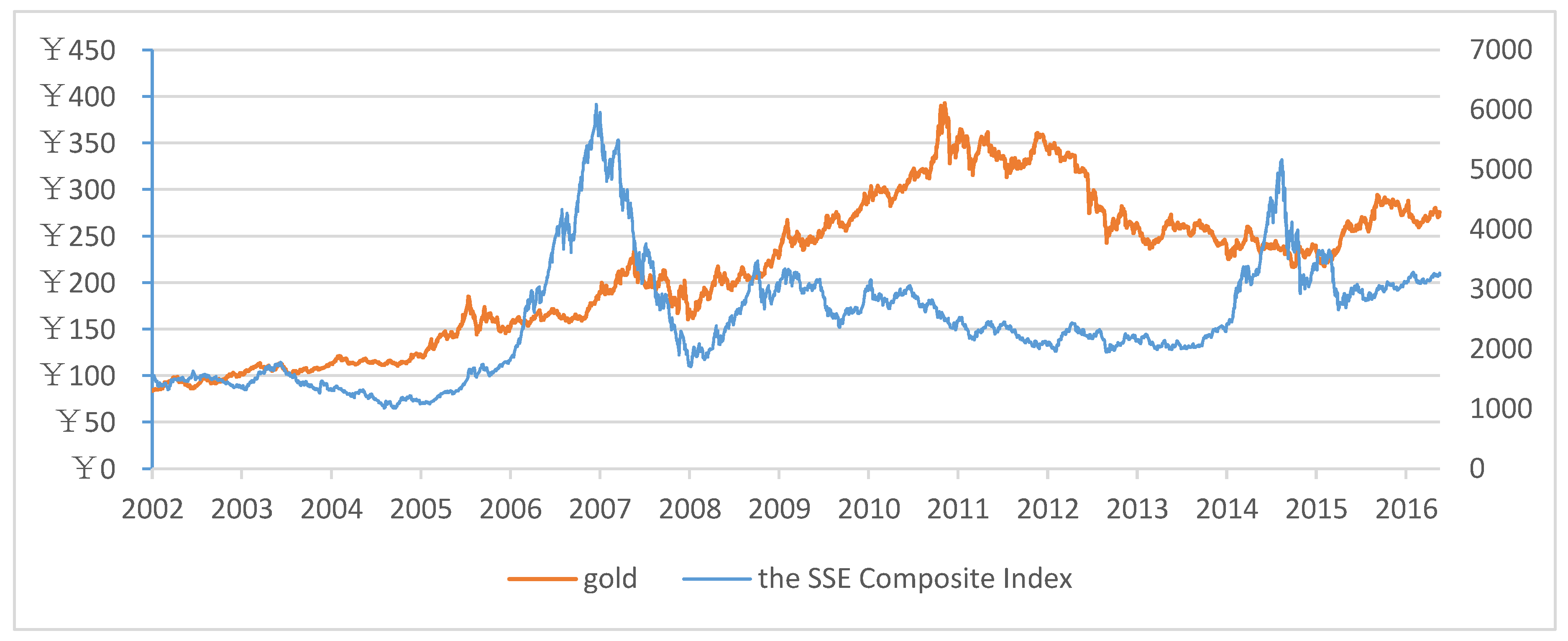
Figure 2.
Gold production and consumption in China (ton) 2009–2016.
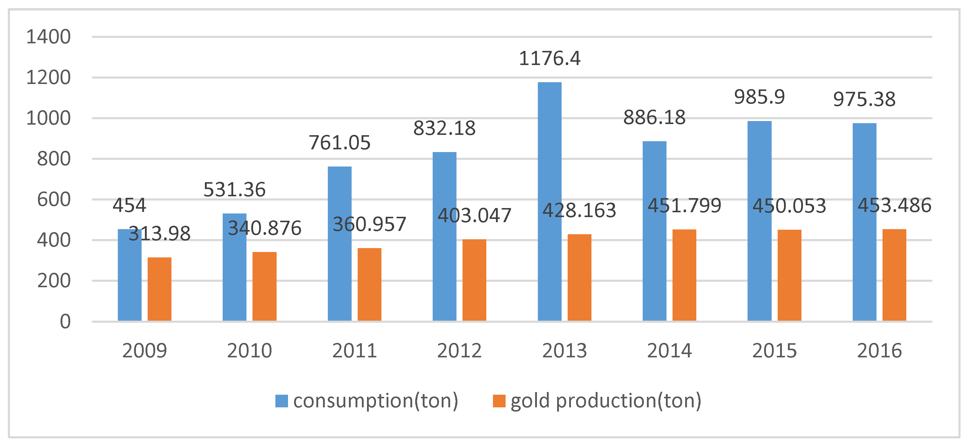
Figure 3.
Five bear markets in China since October 2002.
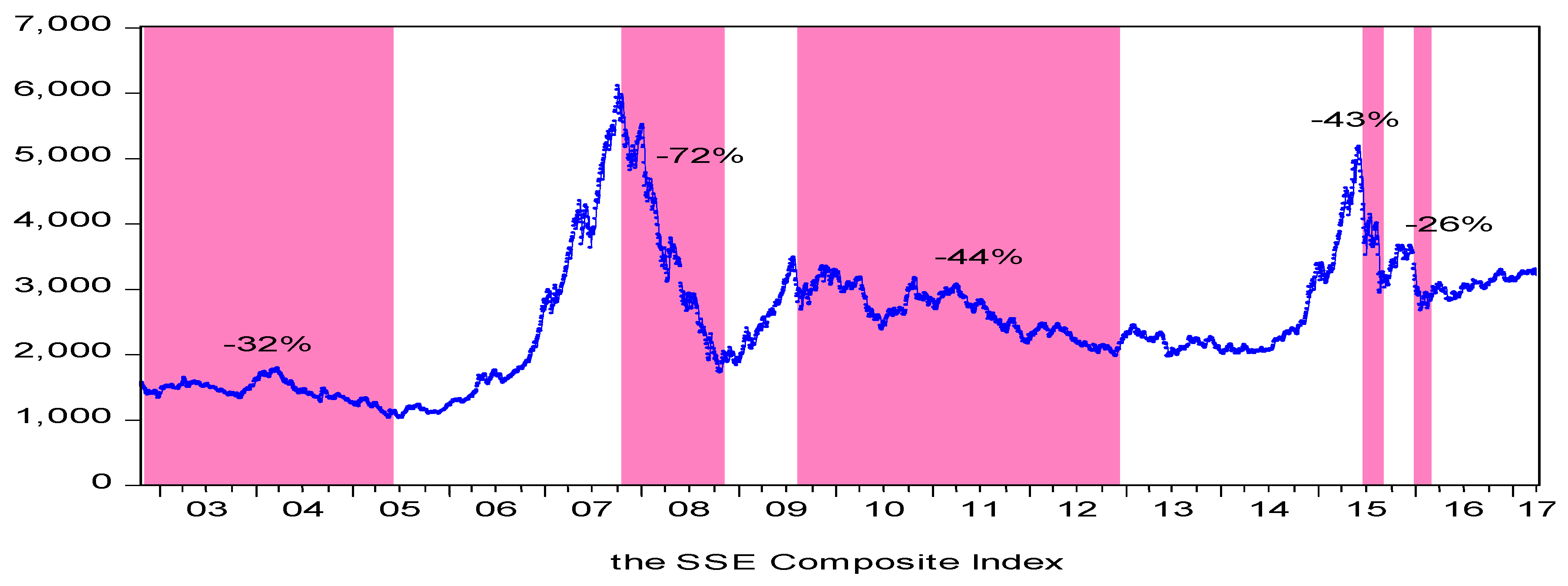
Figure 4.
Return of the Shanghai Stock Exchange Composite Index (31 October 2002–18 April 2017).
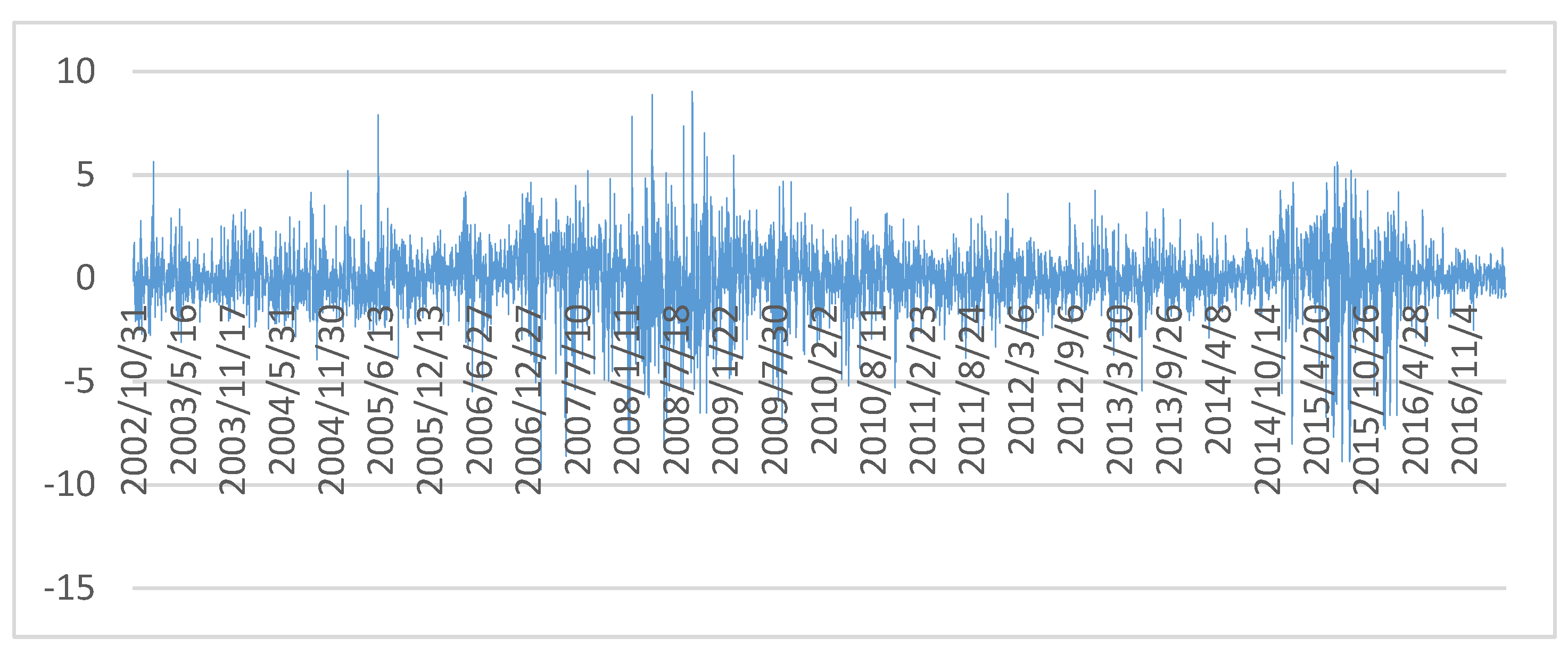
Figure 5.
Return of the Shenzhen Stock Exchange Component Index (31 October 2002–18 April 2017).

Figure 6.
Return of the Capitalization-weighted Stock Index 300 (11 April 2005–18 April 2017).

Figure 7.
Return of the Small and Medium Enterprise Board Index (8 June 2005–18 April 2017).
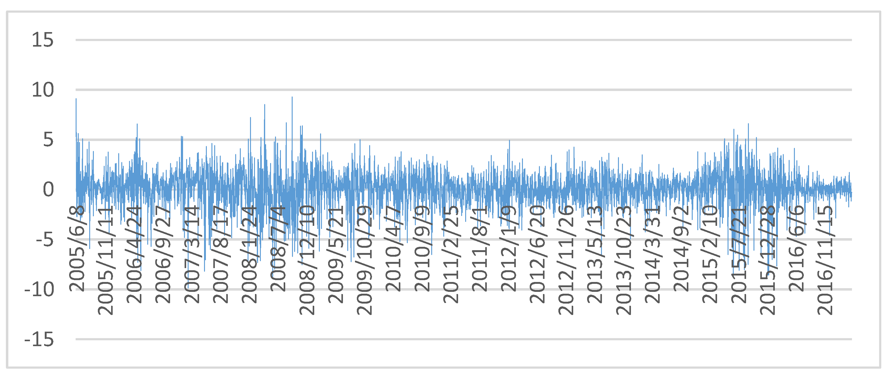
Figure 8.
Return of the Growth Enterprise Market Index (2 June 2010–18 April 2017).
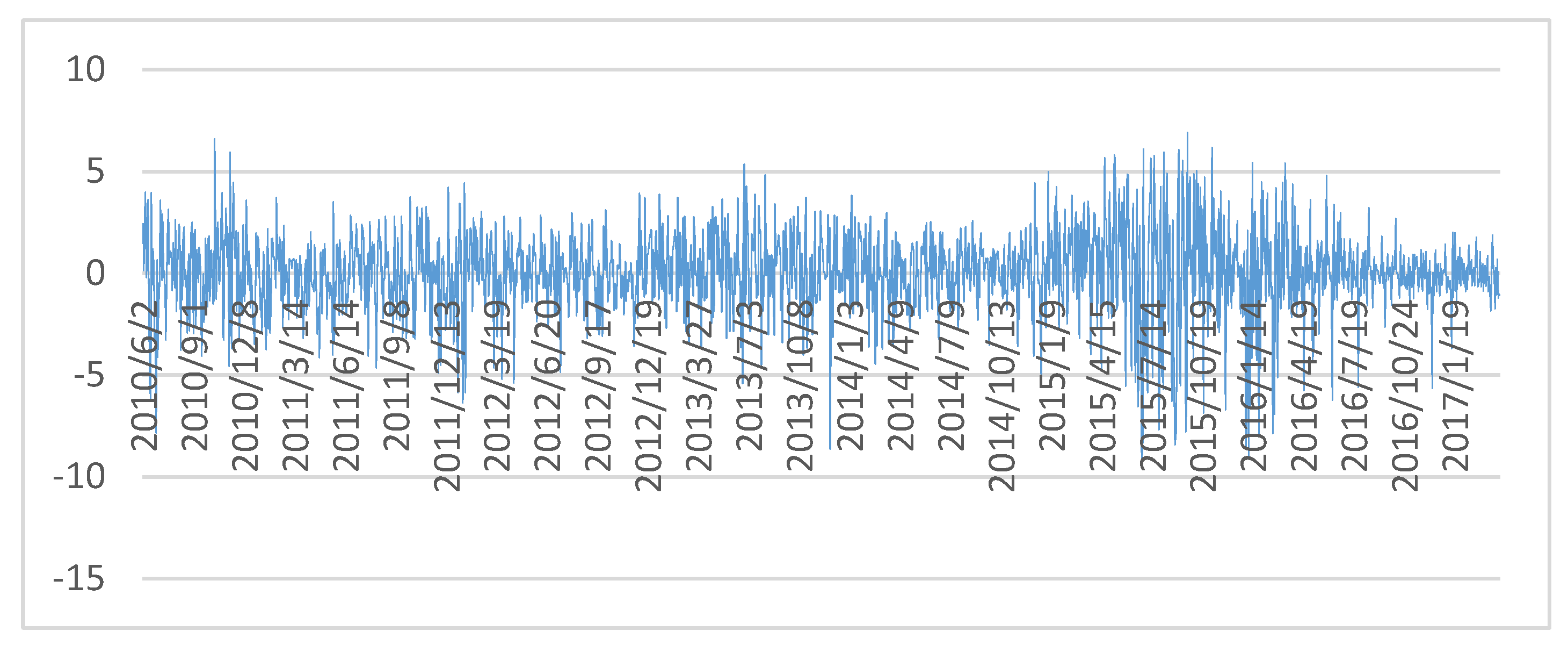
Figure 9.
Return of gold (31 October 2002–18 April 2017).
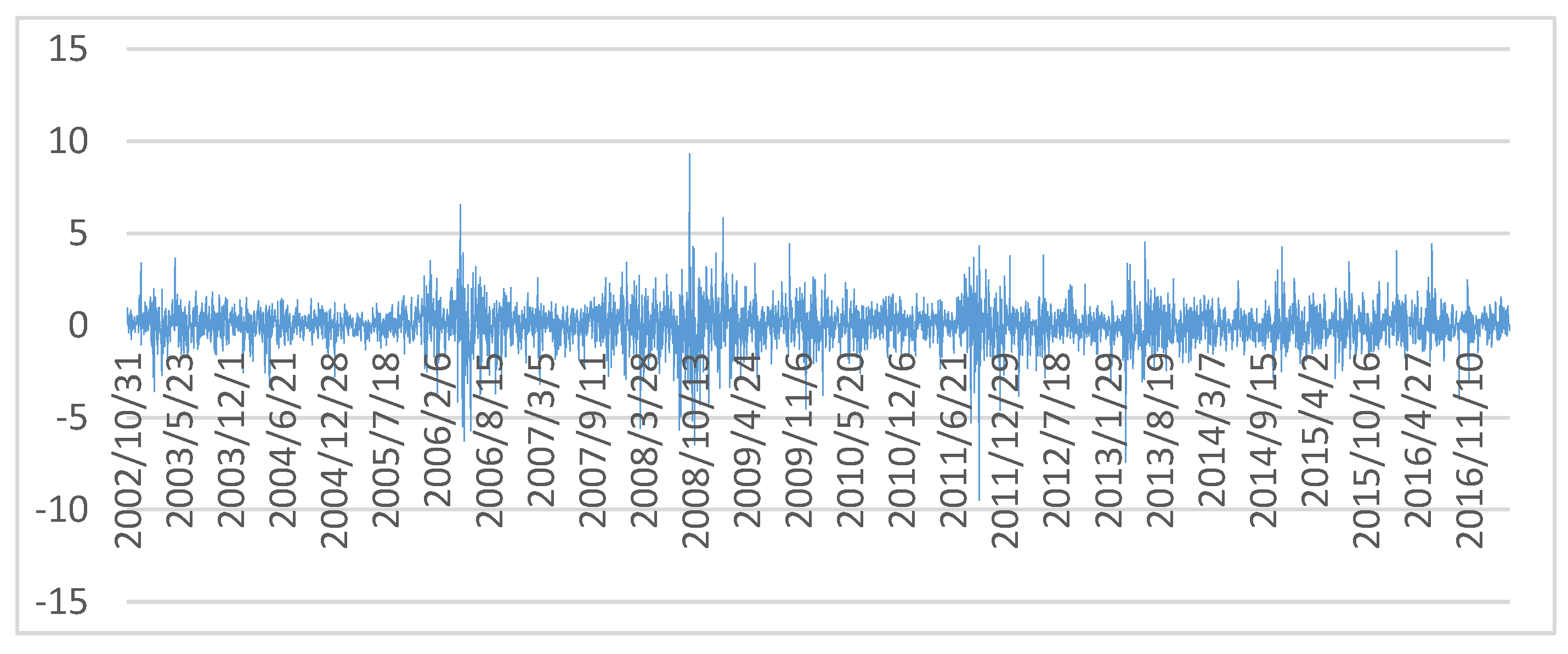
Figure 10.
Dynamic conditional correlations between gold and SSE.
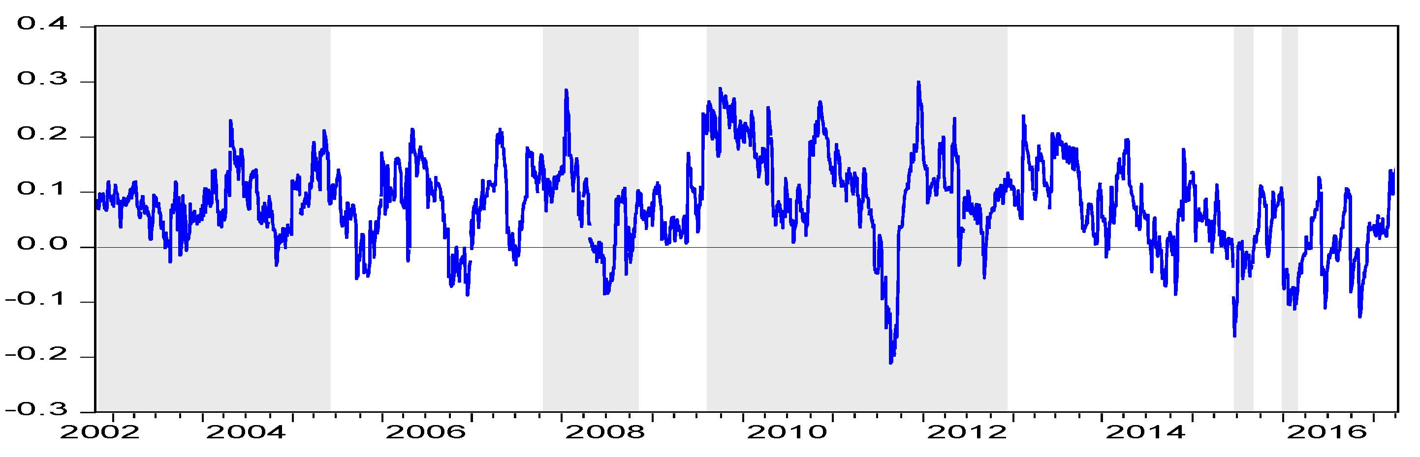
Figure 11.
Dynamic conditional correlations between gold and SZ.

Figure 12.
Dynamic conditional correlations between gold and CSI.

Figure 13.
Dynamic conditional correlations between gold and SME.

Figure 14.
Dynamic conditional correlations between gold and GEM.


Table 1.
The sources and intervals of variables.
| Name | Data Sources | Sample Interval |
|---|---|---|
| Rgold | SGE | 31 October 2002–18 April 2017 |
| Rsse | Datastream | 31 October 2002–18 April 2017 |
| Rsz | Datastream | 31 October 2002–18 April 2017 |
| Rcsi | Datastream | 4 November 2005–18 April 2017 |
| Rsme | Datastream | 8 June 2005–18 April 2017 |
| Rgem | Datastream | 2 June 2010–18 April 2017 |
Note: Rgold, Rsse, Rsz, Rcsi, Rsme, and Rgem represent the return of gold price, the return of the SSE Composite Index, the return of the SZSE Component Index, the return of CSI 300 index, the return of SME Index and the return of GEM Index, respectively.
Table 2.
Descriptive statistics (31 October 2002–18 April 2017) and unit root tests for returns.
| Rsse | Rg(sse) | Rsz | Rg(sz) | Rsci | Rg(sci) | Rsme | Rg(sme) | Rgem | Rg(gem) | |
|---|---|---|---|---|---|---|---|---|---|---|
| Panel A: Descriptive Statistics | ||||||||||
| Mean | 0.021 | 0.035 | 0.035 | 0.035 | 0.042 | 0.031 | 0.066 | 0.032 | 0.038 | 0.004 |
| Median | 0.068 | 0.06 | 0.06 | 0.06 | 0.102 | 0.052 | 0.192 | 0.052 | 0.108 | 0.009 |
| Max | 9.034 | 9.328 | 14.25 | 9.33 | 8.931 | 9.328 | 9.27 | 9.328 | 6.914 | 4.527 |
| Min | −9.256 | −9.474 | −9.75 | −9.47 | −9.695 | −9.474 | −9.87 | −9.474 | −9.332 | −9.474 |
| Std. Dev. | 1.656 | 1.102 | 1.876 | 1.095 | 1.834 | 1.155 | 1.995 | 1.161 | 2.128 | 1.014 |
| Skewness | −0.491 | −0.392 | −0.324 | −0.388 | −0.528 | −0.378 | −0.582 | −0.378 | −0.554 | −0.682 |
| Kurtosis | 7.13 | 10.069 | 6.757 | 10.11 | 6.456 | 9.769 | 5.58 | 9.682 | 4.873 | 11.582 |
| JB | 2637.04 *** | 7402.45 *** | 2120.62 *** | 7463.47 *** | 1589.86 *** | 5648.30 *** | 963.19 *** | 5435.87 *** | 329.39 *** | 5250.75 *** |
| Obs. | 3512 | 3512 | 3502 | 3502 | 2922 | 2922 | 2885 | 2885 | 1669 | 1669 |
| Panel B: Unit Root Test Statistics | ||||||||||
| DF | −57.938 *** | −62.295 *** | −56.115 *** | −62.172 *** | −52.426 *** | −56.584 *** | −50.653 *** | −56.248 *** | −37.577 *** | −43.123 *** |
| ADF | −57.939 *** | −62.323 *** | −56.120 *** | −62.198 *** | −52.441 *** | −56.609 *** | −50.687 *** | −56.278 *** | −37.566 *** | −43.110 *** |
| DF-GLS | −57.603 *** | −62.231 *** | −56.024 *** | −40.748 *** | −9.766 *** | −56.427 *** | −1.939 | −55.255 *** | −4.553 *** | −41.993 *** |
| PP | −57.998 *** | −62.252 *** | −56.229 *** | −62.122 *** | −52.499 *** | −56.582 *** | −50.636 *** | −56.199 *** | −37.501 *** | −43.085 *** |
Notes: JB is the Jarque-Berra test for normality, *** indicates the rejection of null hypotheses at the 1% level. Rgold, Rsse, Rsz, Rcsi, Rsme and Rgem represent the return of gold price, the return of the SSE Composite Index, the return of the SZSE Component Index, the return of CSI 300 index, the return of SME Index and the return of GEM Index, respectively. As the sample intervals of SSE, SZSE, CSI300, SME and GEM are different, the corresponding return of gold price in different sample intervals are also different, which are expressed as Rg(sse), Rg(sz), Rg(sci), Rg(sme) and Rg(gem) respectively.
Table 3.
Ljung-Box Q test and ARCH test statistics.
| Q(10) | ARCH(1) | ARCH(5) | ARCH(10) | |
|---|---|---|---|---|
| Rsse | 37.954 (0.000) *** | 106.269 (0.000) *** | 295.041 (0.000) *** | 352.277 (0.000) *** |
| Rg(sse) | 29.23 (0.001) *** | 99.536 (0.000) *** | 170.455 (0.000) *** | 224.957 (0.000) *** |
| Rsz | 34.332 (0.000) *** | 71.440 (0.000) *** | 215.862 (0.000) *** | 313.094 (0.000) *** |
| Rg(sz) | 33.109 (0.000) *** | 90.553 (0.000) *** | 142.107 (0.000) *** | 178.969 (0.000) *** |
| Rsci | 36.5 (0.000) *** | 83.465 (0.000) *** | 233.190 (0.000) *** | 292.751 (0.000) *** |
| Rg(sci) | 24.404 (0.007) *** | 81.784 (0.000) *** | 137.488 (0.000) *** | 181.913 (0.000) *** |
| Rsme | 25.732 (0.004) *** | 78.634 (0.000) *** | 236.576 (0.000) *** | 278.628 (0.000) *** |
| Rg(sme) | 24.422 (0.007) *** | 78.974 (0.000) *** | 132.345 (0.000) *** | 175.468 (0.000) *** |
| Rgem | 27.884 (0.002) *** | 82.632 (0.000) *** | 205.258 (0.000) *** | 232.847 (0.000) *** |
| Rg(gem) | 9.5233 (0.483) | 74.896 (0.000) *** | 88.509 (0.000) *** | 93.421 (0.000) *** |
Note: Numbers in parenthesis indicate the prob. of the coefficient. *** indicates the rejection of null hypotheses at the 1% level. Rgold, Rsse, Rsz, Rcsi, Rsme and Rgem represent the return of gold price, the return of the SSE Composite Index, the return of the SZSE Component Index, the return of CSI 300 index, the return of SME Index and the return of GEM Index, respectively. As the sample intervals of SSE, SZSE, CSI300, SME and GEM are different, so the corresponding return of gold price in different sample intervals are also different, which are expressed as Rg(sse), Rg(sz), Rg(sci), Rg(sme) and Rg(gem), respectively.
Table 4.
Bear markets in China since October 2002.
| Time Period | Maximum | Minimum | Drop | Origin | |
|---|---|---|---|---|---|
| Bear market I | 31 October 2002–7 June 2005 | 1507.50 | 1030.94 | 32% | Reduction of state-owned shares |
| Bear market II | 16 October 2007–4 November 2008 | 6092.06 | 1706.70 | 72% | The global financial crisis |
| Bear market III | 4 August 2009–3 December 2012 | 3471.44 | 1959.77 | 44% | Restarting IPO, tightening macro policies, the European debt crisis |
| Bear market IV | 12 June 2015–26 August 2015 | 5166.35 | 2927.29 | 43% | De-leveraging, checking OTC Future Financing by the CSRC (China Security Regulatory committee) |
| Bear market V | 22 December 2015–29 February 2016 | 3651.77 | 2687.98 | 26% | Implementing the fuse mechanism and the registration system, devaluation of RMB |
Table 5.
Univariate GARCH (1,1) parameter estimates.
| Coefficient | Std. Error | z-Statistic | Prob. | ||
|---|---|---|---|---|---|
| Rsse | C | 0.014 *** | 0.005 | 2.774 | 0.006 |
| α | 0.058 *** | 0.008 | 7.541 | 0.000 | |
| β | 0.939 *** | 0.007 | 128.774 | 0.000 | |
| Rg(sse) | C | 0.017 *** | 0.004 | 3.794 | 0.000 |
| α | 0.068 *** | 0.009 | 7.264 | 0.000 | |
| β | 0.921 *** | 0.010 | 92.139 | 0.000 | |
| Rsz | C | 0.024 *** | 0.008 | 2.977 | 0.003 |
| α | 0.057 *** | 0.008 | 7.287 | 0.000 | |
| β | 0.938 *** | 0.008 | 119.071 | 0.000 | |
| Rg(sz) | C | 0.016 *** | 0.004 | 3.705 | 0.000 |
| α | 0.064 *** | 0.009 | 7.159 | 0.000 | |
| β | 0.925 *** | 0.010 | 96.013 | 0.000 | |
| Rsci | C | 0.009 * | 0.005 | 1.887 | 0.059 |
| α | 0.056 *** | 0.008 | 7.115 | 0.000 | |
| β | 0.945 *** | 0.007 | 135.173 | 0.000 | |
| Rg(sci) | C | 0.022 *** | 0.006 | 3.620 | 0.000 |
| α | 0.073 *** | 0.011 | 6.614 | 0.000 | |
| β | 0.914 *** | 0.012 | 76.444 | 0.000 | |
| Rsme | C | 0.041 *** | 0.013 | 3.104 | 0.002 |
| α | 0.078 *** | 0.011 | 7.052 | 0.000 | |
| β | 0.914 *** | 0.011 | 85.693 | 0.000 | |
| Rg(sme) | C | 0.024 *** | 0.007 | 3.665 | 0.000 |
| α | 0.071 *** | 0.011 | 6.445 | 0.000 | |
| β | 0.913 *** | 0.012 | 73.841 | 0.000 | |
| Rgem | C | 0.018 | 0.012 | 1.569 | 0.117 |
| α | 0.054 *** | 0.011 | 5.120 | 0.000 | |
| β | 0.943 *** | 0.010 | 94.613 | 0.000 | |
| Rg(gem) | C | 0.038 *** | 0.012 | 3.079 | 0.002 |
| α | 0.074 *** | 0.016 | 4.541 | 0.000 | |
| β | 0.888 *** | 0.023 | 38.610 | 0.000 |
Note: * and *** denote significance at the 10% and 1% level of significance, respectively. Rgold, Rsse, Rsz, Rcsi, Rsme and Rgem represent the return of gold price, the return of the SSE Composite Index, the return of the SZSE Component Index, the return of CSI 300 index, the return of SME Index and the return of GEM Index, respectively. As the sample intervals of SSE, SZSE, CSI300, SME and GEM are different, the corresponding return of gold price in different sample intervals are also different, which are expressed as Rg(sse), Rg(sz), Rg(sci), Rg(sme) and Rg(gem), respectively.
Table 6.
DCC (1,1)–GARCH (1,1) parameter estimates.
| Coef. | S.E | Z | Prob | ||
|---|---|---|---|---|---|
| SSE-Gold | 0.017 *** | 0.006 | 2.944 | 0.003 | |
| 0.957 *** | 0.016 | 60.510 | 0.000 | ||
| SZ-Gold | 0.016 *** | 0.006 | 2.623 | 0.009 | |
| 0.953 *** | 0.019 | 50.333 | 0.000 | ||
| CSI-Gold | 0.045 | 0.028 | 1.599 | 0.110 | |
| 0.770 *** | 0.218 | 3.533 | 0.000 | ||
| SME-Gold | 0.021 ** | 0.009 | 2.252 | 0.024 | |
| 0.947 *** | 0.030 | 31.468 | 0.000 | ||
| GEM-Gold | 0.012 | 0.007 | 1.558 | 0.119 | |
| 0.960 *** | 0.025 | 38.843 | 0.000 |
Note: ** and *** denote significance at the 5% and 1% level of significance, respectively.
Table 7.
The dynamic conditional correlations between stock indexes and gold.
| Bear Markets | Non-Bear Market | |||||
|---|---|---|---|---|---|---|
| I | II | III | IV | V | ||
| SSE-Gold | 0.0808 | 0.0667 | 0.1151 | −0.0410 | −0.0770 | 0.0639 |
| SZ-Gold | 0.0772 | 0.0561 | 0.0926 | −0.0345 | −0.0137 | 0.0612 |
| CSI-Gold | \ | 0.0623 | 0.0870 | 0.0182 | −0.0101 | 0.0669 |
| SME-Gold | \ | 0.0457 | 0.0920 | −0.0424 | −0.0337 | 0.0519 |
| GEM-Gold | \ | \ | 0.0405 | −0.0285 | −0.0278 | 0.0344 |
Note: For convenient observations, the dynamic conditional correlation coefficients (ρ) in the bear markets and non-bear market periods are shown by means of arithmetic average.
Table 8.
DCC (1,1) Model-2 Step Estimation of SSE-GOLD.
| Step One | Step Two | The Mean of Dynamic Conditional Correlations | ||||
|---|---|---|---|---|---|---|
| c | α | β | ||||
| Subsample 1: 31 October 2002–7 June 2005 | ||||||
| SSE | 0.115 (0.074) * | 0.065 (0.003) *** | 0.863 (0.000) *** | −0.026 (0.246) | 0.859 (0.000) *** | 0.0941 |
| GOLD | 0.015 (0.001) *** | 0.056 (0.000) *** | 0.921 (0.000) *** | |||
| Subsample 2: 16 October 2007–4 November 2008 | ||||||
| SSE | 0.079 (0.133) | −0.041 (0.011) ** | 1.035 (0.000) *** | 0.023 (0.318) | 0.958 (0.000) *** | 0.0074 |
| GOLD | 0.068 (0.193) | 0.065 (0.051) * | 0.921 (0.000) *** | |||
| Subsample 3: 4 August 2009–3 December 2012 | ||||||
| SSE | 0.017 (0.012) ** | 0.014 (0.003) *** | 0.974 (0.000) *** | 0.102 (0.107) | 0.694 (0.002) *** | 0.1714 |
| GOLD | 0.020 (0.000) *** | 0.064 (0.000) *** | 0.921 (0.000) *** | |||
| Subsample 4: 12 June 2015–26 August 2015 | ||||||
| SSE | 4.222 (0.849) | −0.039 (0.838) | 0.729 (0.641) | 0.151408 (0.388) | −0.213287 (0.804) | −0.0755 |
| GOLD | 0.082 (0.214) | −0.18245 (0.010) *** | 1.148 (0.000) *** | |||
| Subsample 5: 22 December 2015–29 February 2016 | ||||||
| SSE | 7.035 (0.399) | −0.182 (0.127) | 0.120 (0.919) | −0.065 (0.628) | 0.762 (0.105) | −0.2423 |
| GOLD | 0.259 (0.465) | −0.070 (0.239) | 0.785 (0.014) ** | |||
| Subsample 6: non-bear market | ||||||
| SSE | 0.007 (0.026) ** | 0.059 (0.000) *** | 0.940 (0.000) *** | 0.030 (0.206) | 0.653 (0.007) *** | 0.0701 |
| GOLD | 0.038 (0.000) *** | 0.085 (0.000) *** | 0.884 (0.000) *** | |||
Note: *, ** and *** denote significance at the 10%, 5%, and 1% level of significance, respectively.
Table 9.
DCC (1,1) Model-2 Step Estimation of SZ-GOLD.
| Step One | Step Two | The Mean of Dynamic Conditional Correlations | ||||
|---|---|---|---|---|---|---|
| c | α | β | ||||
| Subsample 1: 31 October 2002–7 June 2005 | ||||||
| SZ | 0.207 (0.103) | 0.069 (0.019) ** | 0.814 (0.000) *** | 0.005 (0.697) | 0.961 (0.000) *** | 0.1065 |
| GOLD | 0.015 (0.001) *** | 0.056 (0.000) *** | 0.921 (0.000) *** | |||
| Subsample 2: 16 October 2007–4 Novemver 2008 | ||||||
| SZ | 0.115 (0.065) * | −0.046 (0.011) ** | 1.037 (0.000) *** | 0.057 (0.236) | 0.849 (0.000) *** | −0.0111 |
| GOLD | 0.050 (0.237) | 0.046 (0.052) * | 0.944 (0.000) *** | |||
| Subsample 3: 4 August 2009–3 December 2012 | ||||||
| SZ | 0.043 (0.043) ** | 0.011 (0.006) *** | 0.972 (0.000) *** | 0.119 (0.033) ** | 0.591 (0.009) *** | 0.1461 |
| GOLD | 0.020 (0.001) *** | 0.063 (0.000) *** | 0.922 (0.000) *** | |||
| Subsample 4: 12 June 2015–26 August 2015 | ||||||
| SZ | 4.555 (0.869) | −0.049 (0.847) | 0.736 (0.685) | −0.192 (/) | 0.976 (/) | −0.0874 |
| GOLD | 0.096 (0.003) *** | −0.214 (0.003) *** | 1.163 (0.000) *** | |||
| Subsample 5: 22 December 2015–29 February 2016 | ||||||
| SZ | 10.267 (0.401) | −0.174 (0.199) | 0.096 (0.936) | −0.210 (/) | 1.051 (/) | −0.4322 |
| GOLD | 0.283 (0.469) | −0.068 (0.257) | 0.757 (0.030) ** | |||
| Subsample 6: non-bear market | ||||||
| SZ | 0.022 (0.000) *** | 0.053 (0.000) *** | 0.940 (0.000) *** | 0.002 (0.912) | 0.716 (0.417) | 0.0682 |
| GOLD | 0.038 (0.000) *** | 0.085 (0.000) *** | 0.884 (0.000) *** | |||
Note: *, ** and *** denote significance at the 10%, 5%, and 1% level of significance, respectively.
Table 10.
DCC (1,1) Model-2 Step Estimation of CSI-GOLD.
| Step One | Step Two | The Mean of Dynamic Conditional Correlations | ||||
|---|---|---|---|---|---|---|
| c | α | β | ||||
| Subsample 1: 16 October 2007–4 November 2008 | ||||||
| CSI | −0.004 (0.979) | −0.035 (0.113) | 1.036 (0.000) *** | 0.049 (0.324) | 0.822 (0.000) *** | −0.0021 |
| GOLD | 0.068 (0.192) | 0.065 (0.051) * | 0.921 (0.000) *** | |||
| Subsample 2: 4 August 2009–3 December 2012 | ||||||
| CSI | 0.028 (0.035) ** | 0.017 (0.004) *** | 0.967 (0.000) *** | 0.136 (0.021) | 0.499 (0.039) | 0.1669 |
| GOLD | 0.020 (0.000) *** | 0.064 (0.000) *** | 0.921 (0.000) *** | |||
| Subsample 3: 12 June 2015–26 August 2015 | ||||||
| CSI | 4.111 (0.863) | 0.029 (0.889) | 0.692 (0.687) | 0.171 (0.355) | 0.209 (0.826) | −0.0973 |
| GOLD | 0.096 (0.003) *** | -0.214 (0.003) *** | 1.163 (0.000) *** | |||
| Subsample 4: 22 December 2015–29 February 2016 | ||||||
| CSI | 5.669 (0.275) | −0.168 (0.127) | 0.206 (0.804) | 0.509 (0.170) | −0.157 (0.283) | −0.2234 |
| GOLD | 0.283 (0.469) | -0.068 (0.257) | 0.757 (0.030) ** | |||
| Subsample 5: non-bear market | ||||||
| CSI | 0.005 (0.107) | 0.055 (0.000) *** | 0.945 (0.000) *** | 0.019 (0.403) | 0.624 (0.039) ** | 0.0663 |
| GOLD | 0.030 (0.000) *** | 0.079 (0.000) *** | 0.895 (0.000) *** | |||
Note: *, ** and *** denote significance at the 10%, 5%, and 1% level of significance, respectively.
Table 11.
DCC (1,1) Model-2 Step Estimation of SME-GOLD.
| Step One | Step Two | The Mean of Dynamic Conditional Correlations | ||||
|---|---|---|---|---|---|---|
| c | α | β | ||||
| Subsample 1: 16 October 2007–4 November 2008 | ||||||
| SME | −0.014 (0.928) | −0.030 (0.085) * | 1.032 (0.000) *** | 0.048 (0.322) | 0.722 (0.006) *** | 0.0043 |
| GOLD | 0.068 (0.193) | 0.065 (0.051) * | 0.921 (0.000) *** | |||
| Subsample 2: 4 August 2009–3 December 2012 | ||||||
| SME | 0.092 (0.047) ** | 0.053 (0.001) *** | 0.910 (0.000) *** | 0.027 (0.110) | 0.941 (0.000) *** | 0.1451 |
| GOLD | 0.020 (0.001) *** | 0.064 (0.000) *** | 0.921 (0.000) *** | |||
| Subsample 3: 12 June 2015–26 August 2015 | ||||||
| SME | 4.263 (0.874) | −0.048 (0.864) | 0.760 (0.656) | −0.033 (/) | 1.037 (/) | −0.1767 |
| GOLD | 0.096 (0.003) *** | -0.214 (0.003) *** | 1.163 (0.000) *** | |||
| Subsample 4: 22 December 2015–29 February 2016 | ||||||
| SME | 9.928 (0.375) | −0.169 (0.205) | 0.098 (0.931) | −0.216 (/) | 1.047 (/) | −0.4166 |
| GOLD | 0.259 (0.465) | −0.070 (0.239) | 0.785 (0.014) ** | |||
| Subsample 5: non-bear market | ||||||
| SME | 0.042 (0.000) *** | 0.065 (0.000) *** | 0.922 (0.000) *** | 0.014 (0.423) | 0.845 (0.000) *** | 0.0585 |
| GOLD | 0.038 (0.000) *** | 0.085 (0.000) *** | 0.884 (0.000) *** | |||
Note: *, ** and *** denote significance at the 10%, 5%, and 1% level of significance, respectively.
Table 12.
DCC (1,1) Model-2 Step Estimation of GEM-GOLD.
| Step One | Step Two | The Mean of Dynamic Conditional Correlations | ||||
|---|---|---|---|---|---|---|
| c | α | β | ||||
| Subsample 1: 4 August 2009–3 December 2012 | ||||||
| GEM | 0.091 (0.139) | 0.038 (0.008) *** | 0.933 (0.000) *** | 0.052 (0.369) | −0.155 (0.769) | 0.0686 |
| GOLD | 0.016 (0.009) *** | 0.068 (0.000) *** | 0.920 (0.000) *** | |||
| Subsample 2: 12 June 2015–26 August 2015 | ||||||
| GEM | 2.950 (0.128) | −0.318 (0.108) | 1.181 (0.000) *** | −0.131 (0.360) | 0.930 (0.000) *** | −0.1414 |
| GOLD | 0.096 (0.003) *** | −0.214 (0.003) *** | 1.163 (0.000) *** | |||
| Subsample 3: 22 December 2015–29 February 2016 | ||||||
| GEM | 8.104 (0.017) ** | −0.210 (0.056) * | 0.466 (0.165) | −0.117 (/) | 1.014 (/) | −0.1418 |
| GOLD | 0.259 (0.465) | −0.070 (0.239) | 0.785 (0.014) ** | |||
| Subsample 4: non-bear market | ||||||
| GEM | 0.018 (0.007) *** | 0.038 (0.000) *** | 0.956 (0.000) *** | −0.013 (/) | −0.001 (/) | 0.0594 |
| GOLD | 0.108 (0.000) *** | 0.122 (0.000) *** | 0.760 (0.000) *** | |||
Note: *, ** and *** denote significance at the 10%, 5%, and 1% level of significance, respectively.
© 2017 by the authors. Licensee MDPI, Basel, Switzerland. This article is an open access article distributed under the terms and conditions of the Creative Commons Attribution (CC BY) license (http://creativecommons.org/licenses/by/4.0/).
Share and Cite
MDPI and ACS Style
Chen, K.; Wang, M. Does Gold Act as a Hedge and a Safe Haven for China’s Stock Market? Int. J. Financial Stud. 2017, 5, 18. https://doi.org/10.3390/ijfs5030018
AMA Style
Chen K, Wang M. Does Gold Act as a Hedge and a Safe Haven for China’s Stock Market? International Journal of Financial Studies. 2017; 5(3):18. https://doi.org/10.3390/ijfs5030018
Chicago/Turabian StyleChen, Ke, and Meng Wang. 2017. "Does Gold Act as a Hedge and a Safe Haven for China’s Stock Market?" International Journal of Financial Studies 5, no. 3: 18. https://doi.org/10.3390/ijfs5030018
Note that from the first issue of 2016, this journal uses article numbers instead of page numbers. See further details here.