Export-Led Growth, Global Integration, and the External Balance of Small Island Developing States


1
US Center, Stockholm Environment Institute, Somerville, MA 02144, USA
2
Cave Hill Campus, University of the West Indies, Cave Hill 64, Barbados
3
Brighton Business School, University of Brighton, Brighton BN2 4AT, UK
*
Author to whom correspondence should be addressed.
Economies 2018, 6(2), 35; https://doi.org/10.3390/economies6020035
Submission received: 5 March 2018
/
Revised: 17 April 2018
/
Accepted: 7 May 2018
/
Published: 4 June 2018
Abstract
:Small, open developing economies in general, and small island developing states (SIDS) in particular, have specific macroeconomic characteristics due both to their openness and their small size. Small size means they can never have fully independent capital-intensive domestic economies, so to raise incomes they must become thoroughly integrated into the global economy. The export sector thus becomes the engine of growth; it provides domestic income, which is spent on domestic goods and imports, driving overall economic output through a multiplier effect. Building on work within the Caribbean structuralist tradition, this paper presents a demand-driven model that includes capital accumulation and external debt. Given the limited data available for many small island states, the model explicitly represents the external macroeconomic balance. An aggregate representation of the national economy is derived formally from a two-sector model, following models of a petroleum exporting country developed Seers and Bruce and Girvan. The model’s performance was evaluated against the historical performance of the Caribbean countries of Barbados, Jamaica and Trinidad and Tobago.
JEL Classification:
B50; F41; O111. Introduction
The economies of small, open, developing states have particular macroeconomic characteristics due to their openness, their economic structure, and their small size. Within this group, many small island developing states (SIDS) are also readily accessible to shipping. The English-speaking Caribbean islands have produced a number of prominent economists who focused attention on those special characteristics, and who had a significant influence over national and regional policy (McKenzie 2005). Lewis (1954, 1979) introduced the idea of a “dual” economy in his analysis of the transformation from largely agrarian economies with abundant labor to industrialized economies. Arguing that domestic capital is scarce, Lewis suggested that countries should seek foreign investors, a strategy since dubbed, somewhat critically, “industrialization by invitation”. In light of subsequent experience, Demas (Demas [1965] 2009) argued that this pathway can only ever lead to a partial transformation. Small economies cannot become “balanced”, with light and heavy manufactures; raw materials production and high technology; and robust agricultural, industrial and service sectors. Rather, they must specialize. Moreover, because beyond a certain point small economies cannot reap the gains of increasing scale on the basis of their own consumption, their specialization must be oriented towards exports. Export-oriented sectors then become leading sectors, in that gross domestic product (GDP) growth tracks export growth to a much greater degree in small economies than it does in large ones.
The theory and policy advocated by Lewis and Demas came under fierce attack as the English-speaking Caribbean islands gained their independence in the 1960s and 1970s. In part, the attack was associated with a self-defined New World Group of young economists (Girvan 2006). One influential model emerging from this group was the Plantation Economy model of Best (1968), of which a central theme was that the export sector in Caribbean countries developed initially to serve a metropolitan economy, and so was not fully integrated into the domestic economy. In a related analysis, Girvan and Girvan (1970) argued that the development and exploitation of mineral resources in small economies by larger ones led to an export sector minimally connected to the rest of the domestic economy. These critiques, although they may have been unduly critical of prior theorists (Figueroa 1996), highlighted the substantial challenges that small economies face in effectively using the export sector to drive a transformation of the domestic economy.
Kraay and Easterly (1999) questioned whether it is appropriate to focus attention on small island economies. They demonstrated that such states tend to have higher GDP per capita compared to their neighbors, and urged instead a focus on landlocked countries. This was not a new observation. Demas (Demas [1965] 2009) echoes a point made by Kuznets (1960) in a classic article, and reinforced recently by Armstrong and Read (1995) that while small size creates problems, it also has benefits, such as unified markets and flexibility, which small states can and have used to their advantage. Kuznets (1960) noted that while country size is inversely related to openness, he found no correlation between size and medium-term economic growth, a finding later confirmed by Milner and Westaway (1993). Nevertheless, although landlocked countries face very serious challenges that should be seriously addressed, SIDS will always be driven by forces out of their direct control. In particular, they rely heavily on export demand and are vulnerable to storms and sea-level rise, which are intensifying with climate change (Nurse et al. 2014). As the countries are too small—in terms of land area and population—to support a self-reliant industrial economy, economic development depends on their integration into a continually changing global economy. Without that integration, increases in GDP per capita are misleading, reflecting what Demas (Demas [1965] 2009) called growth without development. Briguglio (1995) quantified the distinction by comparing country rankings by GDP per capita and vulnerability. Of the 12 Caribbean Community (CARICOM) states included in his study, he found that 11 have an “overrated” GDP per capita (the exception was Trinidad and Tobago). His findings are supported by Guillaumont (2009), and Briguglio’s vulnerability index has informed subsequent efforts to improve the resilience of small states (Lewis-Bynoe 2014). In short, while small island developing states may tend to have comparatively high GDP per capita, it does not secure them a restful existence.1
From the foregoing, we can characterize the economic structure of small island developing states as being composed of one or more export-oriented sectors, which may be capital or labor-intensive, and a domestically oriented labor-intensive sector. Investment goods are imported. SIDS rely heavily on imports, and must thus generate export revenue.
1.1. Related Research
A recurring theme in Caribbean economic thought (Demas [1965] 2009; Best 1968; Girvan and Girvan 1970) is that the foreign exchange earned by the export-oriented sectors must be used to fund the transformation of the rest of the domestic economy. That is, while an effective insertion into the global economy is necessary for development, it must be accompanied by an equally effective insertion of the export-oriented sectors into the domestic economy. The Plantation Economy model of Best was a historical explanation for why this had failed to happen in the Caribbean. Seers (1964) studied domestic-export sector links with a simple model for a small petroleum exporter. He constructed an effective aggregate one-sector model formally from a two-sector model. Bruce and Girvan (1972) later recast his model in Keynesian terms, while following the same strategy. In the models of Seers and Bruce and Girvan, export demand drives domestic demand through a multiplier. The multiplier operates through domestic wage income, which may derive from government employment.
The approach of Seers and Bruce and Girvan is reminiscent of “export base” theory, which enjoyed some popularity in the 1970s. In export base models, local (or “non-basic”) employment or income is a multiplier on the “basic” employment or income generated by export-oriented sectors. In a foundational paper, North (1955) stated explicitly that he meant the theory to apply to U.S. regions or similar and not to developing countries, and most applications of the theory followed his lead. Nevertheless, many of his observations and conclusions are relevant to SIDS: dependence on a narrow range of exports; the need to import capital goods (at least initially); and vulnerability to external demand for the export and changes in the costs of intermediate inputs to production. A distinct difference between U.S. regions and SIDS is that the geographical area covered by the U.S. region can expand, allowing economic activity to diversify, while the geographical extent of small islands is fixed. This distinction was central to both Demas’ (Demas [1965] 2009) and Kuznets’ (1960) arguments.
The models developed in the Caribbean theoretical tradition are structuralist, in that persistent structural features of the economy strongly influence its trajectory (Taylor 2004). Behavior matters, but structuralists argue that economics cannot be reduced to the optimizing behavior of individuals. Rather, institutions and persistent structural features of the economy strongly shape economic behavior. Chenery (1975) in a classic paper, argued that while neoclassical and neo-Marxist theory was originally developed for industrial economies and then later adapted to developing countries, structuralism started with the realities of developing economies. Citing Rosenstein-Rodan (1943), Lewis (1954), and others, he identified the structuralist approach as one that sought to “identify specific rigidities, lags, and other characteristics of the structure of developing economies that affect economic adjustments and the choice of development policy.” While structures are persistent, they can and do change over time, and can sometimes be deliberately altered through policy. Thus, structuralist models may focus on either understanding economic behavior within a given set of structures or the consequences of structural change. In this paper, we take the first approach, as did several authors in the Caribbean structuralist tradition (McKenzie 2005).
Gibson (2003) distinguishes the “early” structuralism of Chenery and others from “late” structuralism as practiced by Taylor and others (Taylor 1989, 1990, 2004; Ocampo 2003; Ocampo et al. 2013), which is more concerned with changes in the global economic environment than was early structuralism. Late structuralism is also concerned with themes explored in this paper: insertion into the global economy, domestic sectoral linkages, and instability (Ocampo 2003). Late structuralist models tend to be demand-led (Setterfield 2002), in that demand drives growth, which stimulates capital accumulation. In contrast, conventional macroeconomic models are typically supply-led, in that capital accumulation drives output growth. It is a truism that exports are particularly important for developing and small open economies because only exports can generate foreign exchange to purchase goods and services that the domestic economy cannot supply. This observation is particularly salient to demand-led models, and demand for exports plays a prominent role in both balance of payments-constrained models (Thirlwall 1979; Hussain 2006, p. 27) and structuralist models (Ocampo et al. 2013, chp. 4). As with Seers (1964), Bruce and Girvan (1972), and the current paper, many structuralist models capture the importance of exports through a multiplier.
The institutional structuralist tradition we draw on in this paper, can be contrasted with the neoclassical models that have dominated macroeconomic theory since the 1970s. The neoclassical “New Structural Economics” arose from the work of Chenery (1975) and others. Theorists in this field encourage countries to climb a technological ladder by following, at each rung, their (possibly dynamic) comparative advantage based on their (developing) endowment (Lin 2012). Similar concerns are shared by the institutional structuralism that informs this paper (e.g., Ocampo 2003), but in a broader institutional context. Because of its narrow context, limited set of causal mechanisms, and specific technical assumptions, institutional structuralists tend to view New Structural Economics as at best incomplete and at worst incoherent (Storm 2015).
Neoclassical growth models have been applied in the Caribbean, of the Solow (1956) and endogenous growth (Aghion et al. 1998) varieties (ECLAC 2009). Such models view growth as arising from expanding provision of factors of production and the productivity with which those factors are used. They posit an aggregate production function subject to decreasing returns to scale that serves to determine the optimal use of factors and the rates at which they are compensated. In the Solow model, productivity growth is exogenous. In endogenous growth models, which allow for constant or increasing returns to scale, firms and workers face a strategic choice between provision (fixed capital investment, labor force participation) and productivity growth (through research and development (R&D) and education or other human capital investment). Their optimal choices determine the growth path of the economy.
Structuralists see several problems with neoclassical growth theory, some of which are acute in the case of SIDS. The focus on supply-side factors ignores the problem of fluctuating demand, while the optimizing framework downplays the substantial uncertainties faced by small economies. Large economies normally operate as going concerns (Means 1964; Lee 1999), so firms can be reasonably confident of the level of demand for their products and the cost of their inputs, given the general state of the economy. That is not the case for SIDS, whose leading firms are small actors in global markets with more or less uncertain downstream demand and upstream prices. Long-range planning is a matter of strategic alliances, contingency planning, flexibility, and responsiveness, not optimal investment plans in a comparatively steady environment. Structuralists also object to the neoclassical production function. In the year after Solow published his model, Phelps Brown (1957) showed that the excellent goodness-of-fit statistics for the Cobb–Douglas production function were due to an accounting identity. Fisher (2005) argued that the neoclassical aggregate production function does not exist, while Samuelson (1966) conceded the claim of Sraffa (1962) and others associated with the University of Cambridge that a marginal productivity of capital cannot be defined (Cohen and Harcourt 2003).2 Phelps Brown’s finding has been rediscovered and reinforced several times (Shaikh 1974; Felipe and McCombie 2001, 2006). These and other critiques of the aggregate production function are thoroughly explored in Felipe and McCombie (2013).
Hausmann and Klinger (2009) provide a unique and compelling viewpoint on the prospects for structural change in the Caribbean. Their empirical approach, grounded in network analysis, sits outside both neoclassical and institutional structural theory. They take global trade data and treat it as a database of technical potential. They ask, first, what export basket a country is producing. They then ask, given the export baskets of other countries, what other products might be considered “nearby”. Their analysis makes clear that the “technological ladder” is a misleading analog. Given a country’s product mix, it can develop in any of several directions. The crucial question is the density of the country’s neighborhood in “product space”; greater density means greater choice. Hausmann and Klinger found that most Caribbean countries, taken individually, are in sparse, peripheral areas of product space.
1.2. Aims and Contribution
In this paper, we present a structuralist model to be applied to small island developing economies. The model was developed in the context of a set of Caribbean climate adaptation scenarios (Drakes et al. 2016) as an exercise in applied economics. The model can be seen as an elaboration of the approach of Seers (1964) and of Bruce and Girvan (1972). As in those papers, the local economy is driven by exports through a multiplier. However, the multiplier operates through both wages in the export sector and export-sector demand for domestic goods. Following Seers and Bruce and Girvan, we explicitly derive the multiplier through formally aggregating a two-sector model. As a consequence, the multiplier is not fixed. This distinguishes the theory in this paper from export base models, at least as practiced in the 1970s, which typically assumed a fixed multiplier (Lewis 1976). When we fit the model to data later in the paper, we estimate parameters related to the underlying two-sector model, rather than directly estimating the multiplier itself.
Data limitations effectively restrict the model to the “external” macroeconomic balance, or the trade gap (Taylor 1989), and only permit an aggregate representation of the national economy. Thus, the model can be used to understand how an exogenous export demand drives the national economy and the external debt, but not to study public spending, central bank operations, and similar internal dynamics. The focus on the external balance is reminiscent of balance of payments-constrained growth models (Thirlwall 1979, 2011), but unlike those models it is meant to apply in the short and medium terms, and not only the long run, so we do not impose a zero trade balance.
Gross domestic product (GDP)3 is driven mainly by exports, although it also responds to changes in population. An import propensity determines the level of imports, while the investment rate depends negatively on debt and positively on utilization of capital. The external balance is then computed, in which net addition to external liabilities is given by the gap between imports and exports, thereby increasing or decreasing the external debt.
We apply the model to three Caribbean countries: Barbados, Jamaica, and Trinidad and Tobago. In doing so, admittedly we break a cardinal rule of structuralism: to construct models tailored to specific national situations and reject “one size fits all” approaches. Our choice largely reflects the constraints of the study for which the model was developed. Macroeconomic analysis was not central; rather, it was one input out of many into the construction of adaptation scenarios at the level of individual islands. The limits of the study informed the decision to use readily-available datasets and focus on the external balance of individual countries. However, there is a further substantive justification for our choice. If the distinctive characteristics of SIDS are ever to be captured in global models, then it will be through stylized models. To the extent that the model presented in this paper succeeds in representing economic trends in these three quite different countries, it could be a step in that direction.
1.3. Study Area
The Caribbean consists of a large number of small island developing states that struggle to enter international markets and become integrated into the global economy. Regional integration, particularly amongst the English-speaking Caribbean countries, has long been seen as a method by which these small economies can play a larger role on the global stage. This has proven extraordinarily difficult, so otherwise modest but successful steps toward integration, such as the formation of the West Indies cricket team, have become important reference points. Political regional integration was first attempted in the late 1950s with the West Indian Federation, but it collapsed within four years. A further attempt began in 1973 with the formation of the Caribbean Community (CARICOM), a regional grouping of 15 Caribbean nations and dependencies, including the three case study countries in this paper.
CARICOM has a set of objectives which include, inter alia, expansion of trade and economic relations with third states and enhanced levels of international competitiveness.4 CARICOM proposes four pillars to achieve these objectives of which the most pertinent is the Caribbean Single Market and Economy (CSME). Hausmann and Klinger’s (2009) study provided strong evidence for the positive potential of integration by showing that CARICOM, in the aggregate, has a high current level of export sophistication and sits in a dense neighborhood of product space. However, integration carries political risks as well as economic rewards, and it is now 17 years since the Revised Treaty of Chaguaramas, which established the process of moving to a CSME. Although there was some early progress (ECLAC 2003), overall achievement is still limited (Alleyne and Francis 2017). Today, countries generally operate independently rather than as a coherent trading bloc when interacting with the rest of the world. Thus, we apply the model separately to each of the three countries vis-à-vis the rest of the world, and do not consider the possibility of regional integration. We briefly describe each case study country in turn.
Barbados is a middle income country according to World Bank definitions. It is the smallest country in our study, with a land area of just 430 square kilometers and a population of less than 0.3 million. Traditionally, the island relied upon sugar production and export; the island was one of the richest European colonies in the Caribbean in the 17th and 18th centuries. At independence in 1966 sugar was still the chief foreign exchange earner; however, the tide was already turning with an increase in visitors from the UK and Canada starting from the 1950s and 1960s continuing with the construction of a deep-water port in 1961 and the growth in international aviation through the 1980s and 1990s. The country is now heavily dependent on the tourist industry. In 2017, visitor exports contributed 13% of GDP directly, 41% of GDP including indirect contributions, and over 68% of all export revenue (WTTC 2018a).
Jamaica is the largest country in the study, with a land area of over 10,000 square kilometres and a population of over 3.0 million. It is also the poorest of our case study countries, with a GDP per capita just over half that of Barbados. Traditionally, the economy was dependent on the production of cash crops for export, predominantly sugar, bananas and tobacco. This changed markedly in the 1950s with the discovery of alumina deposits. Independence in 1962 was followed by sporadic and uneven development. The production and export of agricultural commodities declined, while manufacturing and mining have expanded, first through state assistance programs and then through structural adjustment and economic liberalization programs in the 1980s and 1990s. From the World Bank World Integrated Trade Solution (WITS) database, Jamaica’s key exports today are alumina and bauxite, which together account for almost half of exports. Tourism has also grown, along with remittances, as a substantial source of foreign exchange. Tourism contributed 10% of GDP directly in 2017 and 33% when including indirect contributions (WTTC 2018b). Visitor exports generated over 60% of all exports. Remittances are also a major source of foreign exchange. From the World Bank World Development Indicators (WDI) dataset, they accounted for 17% of GDP in 2016, the 11th highest contribution in the world.
Trinidad and Tobago is the richest of the three case studies, classified as a high income country by the World Bank. It is approximately half the size of Jamaica and has a population of 1.2 million. Its economy is heavily dependent on the extraction and processing of oil and gas. Oil was first discovered in 1866 and the economy has depended on global movements in the price of the commodity ever since (Boopsingh and McGuire 2014). After severe economic distress following the collapse of oil prices in the 1980s, the country began to diversify away from crude oil toward natural gas and derivative products. After a free-trade zone was established in 1988, industries dependent on oil and gas products or inexpensive energy have grown. From the World Bank WITS database, approximately 70% of all exports by value are now from oil or related products. In 2000, an Interim Revenue Stabilisation Fund helped cushion the effects of oil revenue on the economy. The interim fund was formalized in 2007 by an act of Parliament as the Heritage and Stabilisation Fund (Williams 2012).
In the next section we present the two-sector production model. We then aggregate to one sector and add investment and debt dynamics. After calibrating the model for Barbados, Jamaica, and Trinidad and Tobago, we present simulation results for Barbados, discuss the calibrations and simulations, and conclude.
2. Methodology
As discussed in the introduction, we construct a national model by starting from a model with two sectors—export and domestic—and then aggregating. Thus, we assume a dual economic structure, a common feature of models developed in the Caribbean structuralist tradition. The model allows for each sector to have some demand for the other’s outputs. Some products of the export sector might be consumed domestically, whether in final consumption or as an intermediate input to the domestic goods sector, while the domestic sector output might be purchased as intermediate inputs into the export sector, such as domestic services, construction, small manufactures or food production.
The main drivers and feedbacks for the two-sector model are shown in Figure 1. Export demand contributes to GDP and tends to reduce debt levels. GDP both fuels consumption and supplies it, while some consumption adds to imports. Investment also adds to imports, and the gap between imports and exports contributes to debt; remittances also affect debt accumulation.
In keeping with structuralist theory (Taylor 2004), we adopt Kaleckian models of saving and investment. As a matter of accounting, in an open economy, the current account balance B is equal to net saving S (both private and public) less investment,
The balance in this equation is not achieved automatically. Saving and investment decisions are made at different times, and often by different actors, while the current account balance is determined by export demand and domestic demand for imports, whether for consumption, investment, or intermediate inputs to production. In Kaleckian models, capacity utilization affects all three terms, and adjusts to ensure that Equation (1) holds. By contrast, in neoclassical models, flexible prices adjust to bring accounts into balance—we discuss prices below. In the model presented in this paper, and as shown in Figure 1, GDP growth, the debt-to-GDP ratio, and capacity utilization all influence investment, where utilization is determined by the ratio of GDP to the capital stock. The current account balance is computed as the difference between exports and imports, while saving is implicitly determined by income net of expenditure.
2.1. Prices
We express nominal wages and domestic prices in the local currency, and debt and external prices in the world currency, taken to be US dollars (USD). All prices in the model are exogenous, including the exchange rate, e. Exports, imports, and investment goods are all tradable, and we write the corresponding world prices with asterisks. The domestic prices are Px, Pm, and Pi, respectively.
Domestic goods are not traded, and they have only a domestic price, Pd.
For the domestic sector the exogeneity of prices requires some explanation. The price level of consumption, and thus the real wage in the domestic goods sector, is influenced by the cost of imported intermediate and final consumption goods and the wage rates prevailing in the export sector. Holder and Worrell (1985) found, for Barbados, Jamaica, and Trinidad and Tobago, that by far the strongest influence on the price of non-tradables (corresponding to the domestic sector in this model) is the price of tradables (corresponding to the export sector and imported goods in this model). Labor costs had a small and sometimes statistically insignificant effect, while bank lending rates had a statistically significant but not very large effect. In contrast, the lagged price level did explain wage rates. As the prices of tradables are determined in world markets, we assume exogenous prices and implicitly compute wage rates from prices by assuming constant wage shares of income in each production sector.
This approach toward price and wage determination differs from both neoclassical theory, in which prices adjust to bring accounts into balance, and Kaleckian theory, in which prices are set as a markup on labor costs. It is closer in spirit to classical theory with a conventional wage—or, in this case, a conventional wage share (Foley and Michl 1999, p. 104).
To compute the GDP price level P and real GDP Y, we construct a Laspeyre’s index. Denoting exports by X and the share of GDP output going to exports by ξ,
The GDP deflator is equal to a weighted sum of the inflation rate of prices for domestic goods and prices of exports. Using a hat to indicate a growth rate, we have
With this definition, the growth rate of real GDP is computed as
Next we explain how nominal GDP, PY, is determined in the model.
2.2. Gross Domestic Product (GDP) in the Two-Sector Model
Denoting the export sector by a subscript x and the domestic sector by a subscript d, the input–output relationships for the economy relate production Yx, Yd to demand for exports X, domestic consumption of export and domestic goods Cx, Cd, and demand for intermediate goods, net of own-use,
This is a conventional input–output framework, but net of intermediate exchanges within each sector. We expect such exchanges to be present—for example, we expect a demand for domestic goods by the domestic sector—but are compelled by data limitations to restrict the number of free parameters.
On the production side, GDP is equal to the production of goods for export and goods for domestic consumption produced by either the export or domestic-goods sectors,
On the consumption side, total income—GDP plus remittance inflows R plus net new external liabilities eℓ (where e is the exchange rate)—equals total expenditure. Total expenditure is given by consumption of domestically produced goods, PxCx and PdCd, plus consumption of imported goods PmCm and intermediate imports PmmxYx + PmmdYd, plus imported capital goods (investment PiI), and remitted profits Πr,
Net new external liabilities are computed as a residual in the model. Remittance income arrives from a variety of sources, including investment income and remitted wages from family members working abroad. For simplicity, we assume that personal remittance income is proportional to GDP, with a factor ρpers,
Remitted profits (an outflow) represent investment income to overseas investors, which we write as a rate ρK applied to the capital stock valued at the current price of investment goods, Pi,
2.3. Consumption in the Two-Sector Model
All consumption in the model is paid for out of wages or mixed income. Consumption patterns adjust gradually to changes in wages, so rather than the current year’s wage receipts W, consumption is related to (exponentially) smoothed wage income We set a floor to consumption at a basic consumption demand c0 per person, for a population N, and apply a marginal saving rate sw to marginal income above the level needed for basic consumption.
The wage bill, W, is equal to output multiplied by the wage, which we express as wage shares ωx and ωd multiplied by prices in the export and domestic goods sectors,
Basic consumption is supplied fully by the domestic goods sector, while non-basic consumption is split between the consumption of imported goods, with a share m, and consumption of domestically produced goods. Consumption of domestically produced goods is further divided between the consumption of domestic sector goods with a share cd, and of export sector goods with a share cx. The consumption shares sum to one,
With these assumptions, the different components of consumption are given by
Combined, they give total consumption expenditure,
The smoothed wage at the current time step is related to the current wage and the smoothed wage in the previous time step through the relation,
where z is a rate in terms of the time step, which is taken to be a quarter.
Substituting the expressions for consumption, Equations (14) and (15), into the expression for the wage bill, Equation (12), gives
Total imports, M, in domestic currency are given by the sum of imported consumption goods and investment expenditure,
Following Thirlwall (2011, p. 322), we allow imports to depend on the domestic price relative to the price of imports, with an elasticity, εm,5
The expressions above can be combined to construct an aggregate model.
2.4. The Aggregated One-Sector Model
The flow of calculations implied by the two-sector model is shown in Figure 2: exogenous prices, population, and export demand drive the model. Combined with the lagged smoothed wage bill, these variables determine output in each sector, which subsequently determine the instantaneous wage bill. The instantaneous wage then contributes to the next-period lagged smoothed wage bill.
The strategy for constructing the aggregate model is to solve for output from the domestic and export sectors by combining the input–output relations in Equations (6) and (7) with the consumption Equations (14)–(16). Sector output, Yx and Yd, enters the consumption equation through the lagged wage, given by the combination of Equations (12) and (18).
The result is two linear equations in two unknowns. In matrix form, they are
where Φ is a factor translating total final demand to demand for domestic goods,
and θ is the ratio of the domestic price for export goods to the price for domestic goods,
The right-hand side of Equation (22) contains exports X, the previous-period smoothed wage , and the population N; these drive the model, as shown in Figure 2. The coefficients on the left-hand side depend on prices as well as model parameters to be estimated from data.
For notational simplicity, the unwieldy expressions in Equation (22) can be replaced by
where the definitions of the Aij and Ω can be found by comparing this equation to (22). Solving this system gives expressions for real output in the export and domestic goods sectors,
Here, Δ is the determinant of the matrix in Equation (25),
Inserting these expressions into Equation (12), which expresses the wage bill in terms of prices, wage shares, and output, the wage bill can be written as a sum of three terms,
where
When combined with the smoothed wage formula in Equation (18), the aggregate production model is closed.
2.5. Balance of Payments, Debt and Investment
Small size and dependence on export income makes small island developing states prone to external imbalances and fluctuating levels of debt. While in the long run fiscal and financial forces reduce imbalances, thereby ensuring that Thirwall’s Law holds (Thirlwall 1979; Hussain 2006), in the short and medium run significant imbalances are the norm, affecting both daily life and domestic politics. In the model, external debt, D, is denominated in the international currency (USD). Debt is increased by interest accruals at a rate i and net new external liabilities, ℓ,
Net new external liabilities are created whenever imports and net remittance inflows exceed exports, which can be found by subtracting GDP in production terms, Equation (8), from GDP in consumption terms, Equation (9). The result is
Remitted profits depend on the capital stock from Equation (11), while imports include investment goods as in Equation (20). Thus, the external balance is tied to capital accumulation.
Capital stocks in the model follow perpetual inventory dynamics, with the growth rate of the capital stock given by
Here, g = I/K is the gross investment rate and δ is the depreciation rate. Investment decisions are driven by expectations of further real growth, short-term changes in capacity utilization, and debt. Denoting capacity utilization by u, the debt-to-GDP ratio by v and a reference level of v by v*, the gross investment rate is given by
In this expression, the bar over the growth rate of real GDP indicates an exponentially smoothed average. The parameters g0, gu, and gd are all positive. Assuming a constant capital productivity, the utilization growth rate is given by the difference of the GDP growth rate and the growth rate of the capital stock,
2.6. Calibration
The model has been implemented in the Vensim system dynamics (SD) software,6 and we followed recommended procedures for constructing, calibrating and evaluating SD models. In general, SD modelers do not trust any single test as establishing the validity of a model. Rather, a series of tests gradually builds confidence in the model (Forrester and Senge 1980; Martinez-Moyano and Richardson 2013, p. 112). Some of these refer to the model itself: the model structure should be realistic, all parameters should have real-world meanings, and each equation should be logically plausible. We followed these procedures in the model construction documented above. Other confidence-building procedures involve parameter estimation: using data below the level of aggregation of the model whenever possible (Graham 1976, p. 549), estimating each of the model’s components separately (Homer [1983] 2012), and calibrating against historical data (Oliva 2003).
As with many SD models, data limitations prevented us from using data below the level of aggregation of the model, so we followed the other two procedures. Using historical data, we calibrated separately two components: GDP and imports, and investment and debt. Time-series data were collected for Barbados, Jamaica and Trinidad and Tobago from underlying national accounts data used to prepare the Penn World Table version 8.1 (PWT81) (Feenstra et al. 2015), including GDP Y (q_gdp)7, exports X (q_x), imports M (q_m), investment I (q_i), and exchange rates e (xr). Corresponding price levels were computed using nominal values: e.g., the price level of consumption (used as a proxy for Pd) was computed as v_c/q_c, and similarly for the price levels of imports (Pm), exports (Px), investment (Pi), and GDP (P). Exports and GDP were used to compute exports as a share of GDP, ξ. Depreciation rates δ (depr) were taken from the prepared PWT81 tables. To compute debt levels (D), we used the World Bank World Development Indicators (WDI), subtracting reserves (using FI.RES.TOTL.DT.ZS) from external debt stocks (DT.DOD.DECT.CD). Personal remittances as a share of GDP were taken from WDI series BX.TRF.PWKR.DT.GD.ZS. Population data were taken from the United Nations (UN DESA 2015).
To compute capital stocks (K), we first constructed time series from the investment and depreciation data using the perpetual inventory method. This synthetic capital stock time series is determined by investment and depreciation data. It has one free parameter, the initial value for the capital stock, which we estimated by calibrating against the synthetic capital stock time series.
In the perpetual inventory method, the initial capital stock becomes less important over time due to depreciation and growth. Capital stock at time t is computed as
Solving this recurrence relation gives an expression in terms of historical investment and depreciation rates, and the assumed initial value for the capital stock K0, as
The initial value appears in the first term, and is multiplied by an exponentially decaying factor. If it has relative error of ε0 at time 0, by time t the relative error is smaller,
Investment and depreciation data series for Barbados start in 1960, for Jamaica in 1953, and for Trinidad and Tobago in 1950. However, we expect the model parameters to vary (relatively slowly) over time due to structural changes, so we do not calibrate against the full historical data set. Rather, we start the calibration runs in 1986, after several Caribbean countries implemented financial reforms. By that time, a relative error of ±100% is reduced to ±15% in Barbados, ±5% in Jamaica, and ±1% in Trinidad and Tobago. We constructed time series by assuming a capital–output ratio of 2.5 years in the initial year of the capital accounting calculations, but in calibration runs we allowed the 1986 value of the capital stock to vary by the relative errors quoted above.
Following recommended practice in SD modeling, we calibrated separately different sub-models within the full model. We used the Powell (1964) optimizer available in Vensim. For each sub-model, we provided external data series for exports, depreciation rates, prices (including the exchange rate), and population. We then provided additional external data, depending on the sub-model.
We weighted each calibration variable by the inverse mean square root error. With this practice, the errors can be interpreted as confidence intervals, assuming that deviations, as a function of the fitted parameters, are approximately quadratic near the estimated parameter values. Because we do not know the mean square root error a priori, we carried out multiple calibration runs manually, using the estimated errors for the weights, until the estimates converged. This procedure required either one or two iterations.
A complication in calibrating (and running) the model is that we do not impose a requirement that sector receipts cover costs. As a diagnostic, we calculated profit shares as
We then constrained the ranges of the variables ωx, ωd, mx, md, adx and axd such that, aside from acute periods when profits were squeezed, these values were positive in Barbados, Trinidad and Tobago, and in the export sector in Jamaica. It did not prove possible to construct positive profits in the domestic sector in Jamaica given all the other calibration constraints. We note, as a possible source of the discrepancy, that all three price series in Jamaica—Pd, Px, Pm—were equal to each other, unlike in the other two countries. However, in the same period the price levels of consumption and GDP were not constant (Feenstra et al. 2015), suggesting possible problems in the underlying data. In the calibration runs we allowed negative profits in the domestic sector in Jamaica.
2.6.1. GDP and Imports
For GDP, we used the observed data for imports and estimated parameter values for the technical coefficients axd and adx, the base consumption level c0, marginal domestic consumption from exports, cx, saving out of wages sw, the wage smoothing parameter z, initial value for the smoothed wage, and the wage shares ωx and ωd. We used data from 1986 to 2011 for both GDP and exports as a share of GDP for the calibration, but they are not independent, so we estimated 9 parameters using 26 data points.
Imports are tied to GDP through demand for imported intermediate goods for domestic production. Two parameters determine demand for imported consumption goods in Equation (21): the scale parameter m0 and the elasticity εm. To these we add the import coefficients mx and md in Equation (9). Calibrating against import data from 1986 to 2011 gives 4 parameters calibrated against 26 data points.
2.6.2. Investment and Debt
To calibrate the investment function, we provided observed time series for GDP, in addition to the common set of external data. For Jamaica, which has a full debt time series, we also provided debt, D. For Barbados and Trinidad and Tobago, which do not have full debt time series, we used the calculated debt levels. We then estimated values in the investment function, Equation (36): the base investment rate g0, utilization coefficient gu, debt coefficient gd, reference debt-to-GDP level v*, and the initial value for utilization. We also allowed the initial capital stock to vary by the amounts noted above.
For debt, we fit the interest rate, i, initial external debt, and remitted profits as a rate applied to capital, ρK. In both Barbados and Trinidad and Tobago the initial debt level had to be estimated. Furthermore, in Trinidad and Tobago there were substantial changes to the ownership and management structure of the oil and gas sector over 1986–1999 (Boopsingh and McGuire 2014). The structural break appeared to occur near 1997, so we fit two values for the rate of remitted profits, one for before and one for after 1997.
To 26 data points for investment in all countries, we added 12 debt series data points for Barbados and Trinidad. To the 6 investment parameters in all countries, we added 4 debt parameters for Barbados (11 parameters against 38 data points) and 5 debt parameters for Trinidad and Tobago (12 parameters against 38 data points).
In Jamaica, we calibrated investment separately from debt. Fitting the investment data from 1986 to 2011 gave 6 parameters calibrated against 26 data points, while for debt we had 3 parameters against 26 data points.
3. Results
In this section we present goodness-of-fit statistics and estimated parameter values for each of the calibrated models. These are the main results for this paper, as our goal is to document the model and demonstrate its performance against historical data. However, the reason the model was built was to carry out simulations as an input into adaptation scenarios. To illustrate the model for its intended use, we provide some simulation results for Barbados.
3.1. Goodness-of-Fit
We report goodness-of-fit statistics for GDP, investment, debt and imports in Table 1. Particularly problematic values are indicated by underlining. The first three columns in the table are the R2 (coefficient of determination), the adjusted R2, Durbin–Watson, and mean absolute percentage error. The last three columns are the components of a Theil decomposition of the model-data variance (Sterman 1984). The statistic Um is the fraction of the mean squared error due to difference in the mean, Uv is due to differences in variance, and Uc is due to point-to-point covariance. The three values sum to one by construction. Ideally, the model reproduces both the mean and the variance, so the model best reproduces the data series when Uc = 1. The adjusted R2 captures the loss of explanatory power due to the number of parameters relative to the number of observations. It is usually applied to models for the same result variable but with a different number of explanatory variables, but can also be compared to the unadjusted R2 to indicate the bias introduced by having too few data relative to the number of parameters.
Due to the missing debt data in Barbados and Trinidad and Tobago, we used the debt data series mainly to constrain the fit to the investment data, so results for debt are not shown in the table for those two countries. Aside from investment in Trinidad and Tobago, the model performs well on most metrics. We focus on the problematic ones, which are underlined in the table. The Durbin–Watson statistic is less than one for GDP in Barbados, and for GDP and imports in Jamaica, indicating residual serial correlation. The mean absolute percentage errors are generally less than or approximately equal to 10%, aside from investment in Trinidad and Tobago, where it is 15% (and the adjusted R2 statistic is 0.45). The Theil statistics generally suggest fidelity, although there is a bias in the mean value of GDP for Jamaica, and the model does not fully capture variance in investment in Barbados and Trinidad and Tobago, debt in Jamaica, and imports in Barbados and Jamaica.
To gain a better understanding of what the goodness-of-fit statistics represent, an example of a good fit—GDP in Trinidad and Tobago—is shown in Figure 3. An example of a less-good fit—investment in Trinidad and Tobago—is shown in Figure 4. As can be seen, investment generally follows the observed trend, but fails to capture much of the variance, suggesting that factors other than utilization and debt levels significantly influence investment. In Trinidad and Tobago, investment is dominated by the oil and gas industry, and in recent years predominantly by natural gas. Adding lagged natural gas rents as a share of GDP to the model modestly improved the adjusted R2 (to 0.50) and substantially improved the Theil statistics (Uc = 0.92). However, it left essentially unchanged the mean absolute percentage error (MAPE = 14.4).
3.2. Parameter Estimates
Estimated values for selected parameters are shown in Table 2. Some of the values are equal to the imposed upper or lower limit of the allowed range. These are underlined in the table. The estimated parameters are not unreasonable at face value. Investment in Trinidad and Tobago is less sensitive to changes in utilization and debt levels than either Barbados or Jamaica; this is a plausible result, as it is the wealthiest of the three countries and an oil exporter. Jamaica, with the lowest per capita income, has a lower estimated threshold level of debt-to-GDP ratio, which is also plausible.
Domestic consumption of export-sector goods was estimated to be zero in all countries; this is not unreasonable, although it is likely that at least some goods intended for export are consumed domestically. Imports of consumer goods rise with per capita income, although the estimate of zero for Jamaica is problematic (the upper limit of the confidence interval is 0.8%). Wage shares are higher in the domestic sector, but this is because we set different limits; wage shares are allowed to be higher in the domestic sector because they are assumed to be less capital intensive.
The parameter estimates are consistent with considerable intermediate exchange within the national economies between the export and domestic sectors. Indeed, demand for domestic goods by the export sector is at the upper end of the allowed range in each country. This is a positive outcome, if true, because it is indicative of domestic insertion of the export sector. Imports of intermediate goods are lower in the domestic sector than the export sector in all countries, which is reasonable, as the export sectors are more thoroughly integrated into the global economy.
Remitted profits are expected to be higher, the more capital is owned by foreign entities. We thus expect it to be highest in Trinidad and Tobago, and particularly high before the change in the ownership structure. This expectation is met with the estimated parameters. However, the estimate of zero for Barbados is suspect, as the country has seen substantial foreign direct investment, and some profits are remitted.
3.3. Simulations
In the study for which the model was built, simulations were run for all three countries under different regional scenarios. There were two stochastic elements in each run: export demand and storm damage under climate change. For each scenario, the model was run thousands of times to 2050 and mean values were extracted. The storm damage sub-model had some novel elements, and is being documented separately for peer review. As we focus on the performance of the macroeconomic model against historical data, we do not report the study results in this paper. Instead, we demonstrate the model by exploring the consequences of variable export demand for one of the study countries, Barbados.
Historically, demand for exports in Barbados, including tourism demand, has grown at an average of 2.6%/year, with a standard deviation of 12.3%/year8. We ran 25 simulations from 2011 to 2031, in which at each time period the growth rate of export demand was drawn from a truncated normal distribution with the historical mean and standard deviation. The distribution was truncated at ±50%, so that export demand was not allowed to fall or rise by more than half of its previous-period value.
Demographic parameters—crude birth rate, crude death rate, and migration—were drawn from the UN mid-range population projections. Personal remittances per capita were maintained at their 2010 levels, inflated by the GDP price level. Barbados has established and maintained an exchange rate of 2 BBD/USD, and we assumed this level throughout the 20 years of the simulations. World prices for investment, imports, and exports were assumed to grow at 2%/year. Consumer price inflation was calculated using the results of a regression, in which the price inflation depends on the previous period value (with coefficient 0.3) and the GDP per capita growth rate (with coefficient −0.2). Other parameters were set to their calibrated values, as shown in Table 2, and maintained at those values throughout the simulation.
The results are shown in Figure 5, Figure 6 and Figure 7. Each figure shows all 25 simulations, with the first simulation highlighted in order to show one run clearly. Export demand—an exogenous parameter in the model—is shown in Figure 5. As can be seen, the large historical volatility translates in the scenario into a wide range of future possibilities. The highlighted simulation is particularly favorable, but as the figure makes clear, other less positive outcomes are within the range of historical experience.
GDP is shown in Figure 6. The favorable trend in export demand in the highlighted simulation translates into comparatively steady but not spectacular growth. The effect of wage smoothing in the consumption function, persistence in the investment function, and demand for domestic goods makes GDP noticeably less volatile than exports. Nevertheless, export demand ultimately drives the economy. Most simulations lead to positive growth, but in simulations where export demand fails, GDP declines. These scenarios feature a fall in utilization and rising debt, both of which depress investment.
The debt-to-GDP level in Barbados has been generally rising since 2003, although it fell in the immediate aftermath of the 2007 financial crisis. In each simulation, the debt-to-GDP ratio continues to increase, as shown in Figure 7. Under the favorable conditions of the highlighted simulation, the debt-to-GDP ratio stabilizes by 2031. Under less favorable conditions it rises, eventually depressing investment. The model does not automatically stabilize a downward spiral of falling investment and increasing debt; if export demand were to fail consistently, then some intervention would be needed.
Unlike many national economic modeling exercises, the present model was built to provide economic trends in adaptation scenarios, rather than to support economic policy analysis. We reflect on the implications of the model for climate scenarios in the discussion.
4. Discussion
In this paper we have described the development and calibration of a structuralist model for small island developing states (SIDS), which we calibrated against historical data for the Caribbean countries of Barbados, Jamaica, and Trinidad and Tobago. The model design seeks to capture insights from the Caribbean economic tradition while respecting data limitations. We accomplished this by building on that tradition, taking a dual-sector model and constructing an effective one-sector model. This allowed us to calibrate the model against mainly external data, while relating it to an implicit internal structure. For the most part, the estimated parameter values make sense, and the goodness-of-fit statistics are largely supportive of the model.
To the extent that the estimated parameters reflect reality, they yield a positive result about the three economies. A central concern in Caribbean economic thought (emphasized by (Demas [1965] 2009)) is the degree to which the export sector—the source of foreign exchange and the engine of growth—is inserted into the domestic economy. In the model this insertion is reflected in the input–output coefficients adx and axd. These are significantly positive (the bottom end of the 95% confidence interval is greater than zero), indicating substantial intermediate exchange between the domestic and export sectors. The statistical results are also encouraging. The structural features of the Caribbean islands arise from their small size and access to export markets. These features are common to all SIDS, and so is the reality of limited data. This suggests that the model and methods used in this paper might be extended to other SIDS contexts.
Although the results are promising, they must be treated with caution until they have been validated, and the models refined, using data within the countries. Country-specific data can also be used to extend the model for a richer policy discussion. The sectoral detail could be increased, government could be included explicitly, household behavior could be better represented, and the external balance could be coupled with the internal balance. Regarding improvement of the current model, best practice in systems dynamics modeling is to estimate parameters using data below the level of aggregation of the model (Graham 1976, p. 549). Parameters such as domestic consumption of goods from the export sector, cx, basic consumption expenditure c0, and import propensity m can be estimated from household surveys, while consumption of intermediate goods (both domestic and imported) can be estimated from industry surveys and intermittent national statistics. The fundamental assumptions (e.g., the form of the consumption function) can be further tested through surveys. While these data may be available only at discrete times, rather than as a series, point estimates bound the possible range of model parameters and can suggest refinements to the model. Using within-country data, the model can be extended to include domestic activities and the internal balance, including banking, taxation and the government sector.
The model was developed to support a set of Caribbean climate adaptation scenarios (Drakes et al. 2016). At present, the economic models used for climate policy are best suited to large continental economies. Even in this context, they are problematic (Stanton et al. 2009), but by design they are a poor fit to small open economies. Yet, SIDS are particularly vulnerable to climate change (Nurse et al. 2014), so there is a need for models that are well adapted to the realities that SIDS face. As noted by Kraay and Easterly (1999), as a group small open economies, including SIDS, have relatively high per capita incomes compared to countries in the same region. Kraay and Easterly conclude from this that the problems of SIDS and other small states are “small”, but we disagree. In addition to climate vulnerability, SIDS are vulnerable to global and regional economic conditions. They rely for their growth on fickle export markets and for their development on successfully integrating their export and domestic markets. This is not a problem that is solved once and for all, and many of the drivers of change are outside the country’s direct control. Economic models used for policy analysis should account for these facts.
The Shared Socioeconomic Pathways (SSPs) (O’Neill et al. 2014, 2017), part of a new round of global climate scenarios (Moss et al. 2010; Van Vuuren et al. 2014; Ebi et al. 2014) offer a useful language for framing the challenges that SIDS face. The SSPs are organized against axes of “challenges to adaptation” (Rothman et al. 2014) and “challenges to mitigation”. Economic resources are an important component of adaptive capacity. As the simulation results for Barbados indicate, volatile export demand can be a challenge to adaptation for SIDS, and indeed to any small open economy. Prospects for diversification are limited in small states, and for island states both export demand and productive capacity may be affected by climate extremes. As an indication of the potential size of this effect under historical climate, Strobl (2012) has shown that hurricanes have tended to depress GDP per capita growth in the Caribbean by 0.83 percentage points on average. As storms increase in frequency and intensity, the impacts on SIDS are expected to worsen (Nurse et al. 2014). The analysis of technological potential by Hausmann and Klinger (2009) strongly supports the longstanding view of Caribbean economists that regional economic integration can help improve both regional and national economic prospects. However, it remains politically challenging; thus, political constraints are challenges to adaptation in the Caribbean.
In the Caribbean, challenges to adaptation are intertwined with challenges to mitigation. Among the political challenges to integration is the wide difference in economic status, ranging from low-income states to high-income states. Trinidad and Tobago is the wealthiest of the Caribbean nations, a consequence of the country’s successful management of its fossil fuel resources, at least since the 1990s. Yet, the most stringent mitigation pathways are the ones urged by the Association of Small Island States (AOSIS), and even the less restrictive two-degree trajectories imply that most fossil reserves are “unburnable” (McGlade and Ekins 2015). Equity considerations suggest that the wealthiest and historically highest-emitting countries must lead in halting fossil fuel extraction,9 but that is just one consideration in a complex web of equity claims (Lenferna 2018). Serious efforts to meet the Paris agreement could put Trinidad and Tobago’s resources at risk of stranding, and alter the political calculus of regional integration in the Caribbean.
5. Conclusions
This paper presents a macroeconomic model for small island developing states (SIDS) in the Caribbean structuralist tradition. Growth is driven by export demand, while development, in Demas’ (Demas [1965] 2009) terms, is dependent on the integration of the export sector with the rest of the domestic economy. Starting with a two-sector model (domestic and export), we constructed an effective one-sector model and calibrated it for Barbados, Jamaica, and Trinidad and Tobago using components of the external balance, aggregate national accounts, price series, and population.
The results are encouraging. The parameter estimates and goodness-of-fit statistics are, for the most part, reasonable, suggesting that the model is capturing real features of Caribbean economies. The model is intended for use in climate adaptation scenarios, but should be further validated and informed using within-country data. If it proves to be realistic and useful then it should be suitable for other SIDS, both inside and outside the Caribbean.
Author Contributions
E.K.-B., C.D., and T.J.L. developed the conceptual structure for the model. E.K.-B. implemented it in Vensim. E.K.-B. wrote the paper with input from C.D. and T.J.L.
Funding
The Global to Local Caribbean Climate Change Adaptation and Mitigation Scenarios (GoLoCarSce) research project was partially funded (Contract Number: FED/2011/281-134) by the European Union-African, Caribbean and Pacific (ACP) Research Programme for Sustainable Development (CP-RSD). Further funding was provided by the International Development Research Centre (IDRC) under the Sustainable Water Management under Climate Change in Small Island States of the Caribbean Grant 107096-001. The results can under no circumstances be regarded as reflecting the position of the European Union or IDRC.
Acknowledgments
The authors would like to thank John Agard and Adrian Cashman for their support and critique. We are grateful to Winston Moore for his critical review of the model at an early stage, and to the participants of two scenario workshops, who made extensive and helpful comments on the overall modeling approach and specific details. The authors take full responsibility for whatever errors or misconceptions may remain.
Conflicts of Interest
The authors declare no conflict of interest.
References
- Aghion, Philippe, Peter Howitt, and Cecilia García-Peñalosa. 1998. Endogenous Growth Theory. Cambridge: MIT Press. [Google Scholar]
- Alleyne, Antonio, and Brian M. Francis. 2017. Globalisation and International Competitiveness: The Future of the Caribbean Require Reform Changes. SSRN Scholarly Paper ID 2956746. Rochester: Social Science Research Network. Available online: http://papers.ssrn.com/abstract=2956746 (accessed on 8 November 2015).
- Armstrong, Harvey, and Robert Read. 1995. Western European Micro-States and EU Autonomous Regions: The Advantages of Size and Sovereignty. World Development 23: 1229–45. [Google Scholar] [CrossRef]
- Bates, Samuel, and Valérie Angeon. 2015. Promoting the Sustainable Development of Small Island Developing States: Insights from Vulnerability and Resilience Analysis. Région et Développement 42: 15–29. [Google Scholar]
- Best, Lloyd A. 1968. Outlines of a Model of Pure Plantation Economy. Social and Economic Studies 17: 283–326. Available online: http://www.jstor.org/stable/27856339 (accessed on 23 June 2015).
- Boopsingh, Trevor M., and Gregory McGuire, eds. 2014. From Oil to Gas and Beyond: A Review of the Trinidad and Tobago Model and Analysis of Future Challenges. Lanham: University Press of America. [Google Scholar]
- Briguglio, Lino. 1995. Small Island Developing States and Their Economic Vulnerabilities. World Development 23: 1615–32. [Google Scholar] [CrossRef]
- Bruce, Carlton J., and Cherita Girvan. 1972. The Open Petroleum Economy: A Comparison of Keynesian and Alternative Formulations. Social and Economic Studies 21: 125–52. Available online: http://www.jstor.org/stable/27856525 (accessed on 8 August 2015).
- Chenery, Hollis B. 1975. The Structuralist Approach to Development Policy. The American Economic Review 65: 310–16. Available online: http://www.jstor.org/stable/1818870 (accessed on 4 November 2014).
- Cohen, Avi J., and Geoffrey C. Harcourt. 2003. Retrospectives: Whatever Happened to the Cambridge Capital Theory Controversies? Journal of Economic Perspectives 17: 199–214. Available online: http://www.jstor.org/stable/3216846 (accessed on 27 August 2012). [CrossRef]
- Demas, William G. 2009. The Economics of Development in Small Countries: With Special Reference to the Caribbean. Kingston and St. Michael: University of the West Indies Press. First published 1965. [Google Scholar]
- Drakes, Crystal, Timothy Laing, Eric Kemp-Benedict, and Adrian Cashman. 2016. Caribbean Scenarios 2050. CERMES Technical Report, 84. Cave Hill, Barbados: Centre for Resource Management and Environmental Studies, University of the West Indies. [Google Scholar]
- Ebi, Kristie L., Tom Kram, Detlef P. van Vuuren, Brian C. O’Neill, and Elmar Kriegler. 2014. A New Toolkit for Developing Scenarios for Climate Change Research and Policy Analysis. Environment: Science and Policy for Sustainable Development 56: 6–16. [Google Scholar] [CrossRef]
- ECLAC. 2003. Progress Made in the Implementation of the CARICOM Single Market and Economy. LC/CAR/G.770. Port of Spain: Economic Commission for Latin America and the Caribbean, United Nations. [Google Scholar]
- ECLAC. 2009. Economic Growth in the Caribbean. LC/CAR/L.244. Port of Spain: Economic Commission for Latin America and the Caribbean, United Nations. [Google Scholar]
- Feenstra, Robert C., Robert Inklaar, and Marcel P. Timmer. 2015. The next Generation of the Penn World Table. American Economic Review 105: 3150–82. [Google Scholar] [CrossRef]
- Felipe, Jesus, and John S. L. McCombie. 2001. The CES Production Function, the Accounting Identity, and Occam’s Razor. Applied Economics 33: 1221–32. [Google Scholar] [CrossRef]
- Felipe, Jesus, and John McCombie. 2006. The Tyranny of the Identity: Growth Accounting Revisited. International Review of Applied Economics 20: 283–99. [Google Scholar] [CrossRef]
- Felipe, Jesus, and John S. L. McCombie. 2013. The Aggregate Production Function and the Measurement of Technical Change: “Not Even Wrong”. Cheltenham: Edward Elgar. [Google Scholar]
- Figueroa, Mark. 1996. The Plantation School and Lewis: Contradictions, Continuities and Continued Caribbean Relevance. Social and Economic Studies 45: 23–49. Available online: http://www.jstor.org/stable/27866101 (accessed on 23 June 2015).
- Fisher, Franklin M. 2005. Aggregate Production Functions—A Pervasive, but Unpersuasive, Fairytale. Eastern Economic Journal 31: 489–91. Available online: http://www.jstor.org/stable/40326426 (accessed on 17 December 2017).
- Foley, Duncan K., and Thomas R. Michl. 1999. Growth and Distribution. Cambridge: Harvard University Press. [Google Scholar]
- Forrester, Jay W., and Peter M. Senge. 1980. Tests for Building Confidence in System Dynamics Models. System Dynamics, TIMS Studies in Management Sciences 14: 209–28. [Google Scholar]
- Gibson, Bill. 2003. An Essay on Late Structuralism. In Development Economics and Structuralist Macroeconomics: Essays in Honor of Lance Taylor. Edited by Amitava Krishna Dutt and Jaime Ros. Cheltenham: Edward Elgar, pp. 52–76. Available online: http://www.uvm.edu/~wgibson/Research/tay.pdf (accessed on 3 November 2014).
- Girvan, Cherita, and Norman Girvan. 1970. Multinational Corporations and Dependent Underdevelopment in Mineral-Export Economies. Social and Economic Studies 19: 490–526. Available online: http://www.jstor.org/stable/27856449 (accessed on 8 August 2015).
- Girvan, Norman. 2006. Caribbean Dependency Thought Revisited. Canadian Journal of Development Studies/Revue Canadienne d’études Du Développement 27: 328–52. [Google Scholar] [CrossRef]
- Graham, Alan K. 1976. Parameter Formulation and Estimation in System Dynamics Models. Paper presented at the 1976 International Conference on System Dynamics Method, Geilo, Norway, August 8–15; pp. 541–80. [Google Scholar]
- Guillaumont, Patrick. 2009. An Economic Vulnerability Index: Its Design and Use for International Development Policy. Oxford Development Studies 37: 193–228. [Google Scholar] [CrossRef] [Green Version]
- Hausmann, Ricardo, and Bailey Klinger. 2009. Policies for Achieving Structural Transformation in the Caribbean. Discussion Paper 2, Private Sector Development Discussion Paper. Washington, DC, USA: Inter-American Development Bank. [Google Scholar]
- Holder, Carlos, and DeLisle Worrell. 1985. A Model of Price Formation for Small Economies: Three Caribbean Examples. Journal of Development Economics 18: 411–28. [Google Scholar] [CrossRef]
- Homer, Jack B. 2012. Partial-Model Testing as a Validation Tool for System Dynamics. System Dynamics Review 28: 281–94. [Google Scholar] [CrossRef]
- Hussain, Mohammed Nureldin. 2006. The Implications of Thirlwall’s Law for Africa’s Development Challenges. In Growth and Economic Development: Essays in Honour of A.P. Thirlwall. Edited by Philip Arestis, John McCombie and Roger Vickerman. Cheltenham: Edward Elgar Publishing Limited. [Google Scholar]
- Kraay, Aart, and William Easterly. 1999. Small States, Small Problems? Washington, DC: The World Bank, Available online: http://elibrary.worldbank.org/doi/book/10.1596/1813-9450-2139 (accessed on 19 January 2016).
- Kuznets, Simon. 1960. Economic Growth of Small Nations. In Economic Consequences of the Size of Nations. Edited by Austin E. Robinson. London: Palgrave Macmillan, pp. 14–32. [Google Scholar] [CrossRef]
- Lee, Frederic S. 1999. Post Keynesian Price Theory. Cambridge: Cambridge University Press. [Google Scholar]
- Lenferna, Georges Alexandre. 2018. Can We Equitably Manage the End of the Fossil Fuel Era? Energy Research & Social Science 35: 217–23. [Google Scholar] [CrossRef]
- Lewis, W. Arthur. 1954. Economic Development with Unlimited Supplies of Labour. The Manchester School 22: 139–91. [Google Scholar] [CrossRef]
- Lewis, W. Arthur. 1979. The Dual Economy Revisited. The Manchester School 47: 211–29. [Google Scholar] [CrossRef]
- Lewis, W. Cris. 1976. Export Base Theory and Multiplier Estimation: A Critique. The Annals of Regional Science 10: 58–70. [Google Scholar] [CrossRef]
- Lewis-Bynoe, Denny, ed. 2014. Building the Resilience of Small States: A Revised Framework. London: Commonwealth Secretariat. [Google Scholar]
- Lin, Justin Yifu, ed. 2012. New Structural Economics: A Framework for Rethinking Development and Policy. Washington, DC: The World Bank, Available online: http://elibrary.worldbank.org/doi/book/10.1596/978-0-8213-8955-3 (accessed on 7 October 2015).
- Martinez-Moyano, Ignacio J., and George P. Richardson. 2013. Best Practices in System Dynamics Modeling. System Dynamics Review 29: 102–23. [Google Scholar] [CrossRef]
- McGlade, Christophe, and Paul Ekins. 2015. The Geographical Distribution of Fossil Fuels Unused When Limiting Global Warming to 2 °C. Nature 517: 187–90. [Google Scholar] [CrossRef] [PubMed]
- McKenzie, Rex A. 2005. Structuralist Approaches to Social & Economic Development in the English Speaking Caribbean. Paper presented at the 6th Annual SALISES Conference on Governance, Institutions and Economic Growth: Reflections on Sir Arthur Lewis’ Theory of Economic Growth, Mona, Jamaica, March 17; Available online: http://eprints.kingston.ac.uk/36115/ (accessed on 7 April 2018).
- Means, Gardiner. 1964. The Corporate Revolution in America. Springfield: Collier Books. [Google Scholar]
- Milner, Chris, and Tony Westaway. 1993. Country Size and the Medium-Term Growth Process: Some Cross-Country Evidence. World Development 21: 203–11. [Google Scholar] [CrossRef]
- Moss, Richard H., Jae A. Edmonds, Kathy A. Hibbard, Martin R. Manning, Steven K. Rose, Detlef P. van Vuuren, Timothy R. Carter, Seita Emori, Mikiko Kainuma, Tom Kram, and et al. 2010. The next Generation of Scenarios for Climate Change Research and Assessment. Nature 463: 747–56. [Google Scholar] [CrossRef] [PubMed]
- North, Douglass C. 1955. Location Theory and Regional Economic Growth. Journal of Political Economy 63: 243–58. Available online: http://www.jstor.org.ezproxy.library.tufts.edu/stable/1825076 (accessed on 21 March 2018). [CrossRef]
- Nurse, Leonard A., Roger F. McLean, John Agard, Lino P. Briguglio, Virginie Duvat-Magnan, Netatua Pelesikoti, Emma Tompkins, and Arthur Webb. 2014. Small Islands. In Climate Change 2014: Impacts, Adaptation, and Vulnerability. Part B: Regional Aspects. Contribution of Working Group II to the Fifth Assessment Report of the Intergovernmental Panel of Climate Change. Edited by Vicente R. Barros, Christopher B. Field, David Jon Dokken, Michael D. Mastrandrea, Katharine J. Mach, T. Eren Bilir, Monalisa Chatterjee, Kristie L. Ebi, Yuka Otsuki Estrada, Robert C. Genova and et al. Cambridge and New York: Cambridge University Press, pp. 1613–54. [Google Scholar]
- Ocampo, José Antonio. 2003. Structural Dynamics and Economic Growth in Developing Countries. Santiago: United Nations Economic Commission for Latin America and the Caribbean (ECLAC). [Google Scholar]
- Ocampo, José Antonio, Codrina Rada, and Lance Taylor. 2013. Growth and Policy in Developing Countries: A Structuralist Approach. New York: Columbia University Press. [Google Scholar]
- Oliva, Rogelio. 2003. Model Calibration as a Testing Strategy for System Dynamics Models. European Journal of Operational Research 151: 552–68. [Google Scholar] [CrossRef]
- O’Neill, Brian C., Elmar Kriegler, Kristie L. Ebi, Eric Kemp-Benedict, Keywan Riahi, Dale S. Rothman, Bas J. van Ruijven, Detlef P. van Vuuren, Joern Birkmann, Kasper Kok, and et al. 2017. The Roads Ahead: Narratives for Shared Socioeconomic Pathways Describing World Futures in the 21st Century. Global Environmental Change 42: 169–80. [Google Scholar] [CrossRef]
- O’Neill, Brian C., Elmar Kriegler, Keywan Riahi, Kristie L. Ebi, Stephane Hallegatte, Timothy R. Carter, Ritu Mathur, and Detlef P. Vuuren. 2014. A New Scenario Framework for Climate Change Research: The Concept of Shared Socioeconomic Pathways. Climatic Change 122: 387–400. [Google Scholar] [CrossRef]
- Phelps Brown, E. H. 1957. The Meaning of the Fitted Cobb-Douglas Function. The Quarterly Journal of Economics 71: 546–60. [Google Scholar] [CrossRef]
- Powell, J. D. Michael. 1964. An Efficient Method for Finding the Minimum of a Function of Several Variables without Calculating Derivatives. The Computer Journal 7: 155–62. [Google Scholar] [CrossRef]
- Rosenstein-Rodan, N. Paul. 1943. Problems of Industrialisation of Eastern and South-Eastern Europe. The Economic Journal 53: 202–11. Available online: http://www.jstor.org/stable/2226317 (accessed on 12 August 2010).
- Rothman, Dale S., Patricia Romero-Lankao, Vanessa J. Schweizer, and Beth A. Bee. 2014. Challenges to Adaptation: A Fundamental Concept for the Shared Socio-Economic Pathways and Beyond. Climatic Change 122: 495–507. [Google Scholar] [CrossRef]
- Samuelson, Paul A. 1966. A Summing Up. The Quarterly Journal of Economics 80: 568–83. [Google Scholar] [CrossRef]
- Seers, Dudley. 1964. The Mechanism of an Open Petroleum Economy. Social and Economic Studies 13: 233–42. Available online: http://www.jstor.org/stable/27853782 (accessed on 8 August 2015).
- Setterfield, Mark, ed. 2002. The Economics of Demand-Led Growth: Challenging the Supply-Side Vision of the Long Run. Cheltenham and Northampton: Edward Elgar. [Google Scholar]
- Shaikh, Anwar. 1974. Laws of Production and Laws of Algebra: The Humbug Production Function. The Review of Economics and Statistics 56: 115–20. [Google Scholar] [CrossRef]
- Solow, Robert M. 1956. A Contribution to the Theory of Economic Growth. The Quarterly Journal of Economics 70: 65–94. [Google Scholar] [CrossRef]
- Sraffa, Piero. 1962. Production of Commodities: A Comment. The Economic Journal 72: 477–79. [Google Scholar] [CrossRef]
- Stanton, Elizabeth A., Frank Ackerman, and Sivan Kartha. 2009. Inside the Integrated Assessment Models: Four Issues in Climate Economics. Climate and Development 1: 166–84. [Google Scholar] [CrossRef]
- Sterman, John D. 1984. Appropriate Summary Statistics for Evaluating the Historical Fit of System Dynamics Models. Dynamica 10: 51–66. [Google Scholar]
- Storm, Servaas. 2015. Structural Change. Development and Change 46: 666–99. [Google Scholar] [CrossRef]
- Strobl, Eric. 2012. The Economic Growth Impact of Natural Disasters in Developing Countries: Evidence from Hurricane Strikes in the Central American and Caribbean Regions. Journal of Development Economics 97: 130–41. [Google Scholar] [CrossRef]
- Stubbs, Richard. 1999. War and Economic Development: Export-Oriented Industrialization in East and Southeast Asia. Comparative Politics 31: 337–55. [Google Scholar] [CrossRef]
- Taylor, Lance. 1989. Stabilization and Growth in Developing Countries: A Structuralist Approach. Chur: Taylor & Francis. [Google Scholar]
- Taylor, Lance, ed. 1990. Socially Relevant Policy Analysis: Structuralist Computable General Equilibrium Models for the Developing World. Cambridge: MIT Press. [Google Scholar]
- Taylor, Lance. 2004. Reconstructing Macroeconomics: Structuralist Proposals and Critiques of the Mainstream. Cambridge: Harvard University Press. [Google Scholar]
- Thirlwall, Anthony Philip. 1979. The Balance of Payments Constraint as an Explanation of International Growth Rate Differences. BNL Quarterly Review 32: 45–53. [Google Scholar]
- Thirlwall, Anthony Philip. 2011. Balance of Payments Constrained Growth Models: History and Overview. PSL Quarterly Review 64: 307–51. Available online: http://papers.ssrn.com/abstract=2049740 (accessed on 13 March 2015).
- UN DESA. 2015. World Population Prospects: The 2015 Revision. New York: United Nations, Department of Economic and Social Affairs, Population Division. [Google Scholar]
- Van Vuuren, Detlef P., Elmar Kriegler, Brian C. O’Neill, Kristie L. Ebi, Keywan Riahi, Timothy R. Carter, Jae Edmonds, Stephane Hallegatte, Tom Kram, Ritu Mathur, and et al. 2014. A New Scenario Framework for Climate Change Research: Scenario Matrix Architecture. Climatic Change 122: 373–86. [Google Scholar] [CrossRef]
- Williams, Ewart. 2012. Review of the Heritage and Stabilisation Fund (HSF). Paper presented at the Revenue Management in Hydrocarbon Economies, University of the West Indies, St. Augustine, Trinidad and Tobago, June 21; Available online: http://sta.uwi.edu/conferences/12/revenue/documents/GovernorPresentationReviewHSFUWIJune21.pdf (accessed on 23 March 2015).
- WTTC. 2018a. Travel & Tourism Economic Impact 2018 Barbados. London: World Travel and Tourism Council. [Google Scholar]
- WTTC. 2018b. Travel & Tourism Economic Impact 2018 Jamaica. London: World Travel and Tourism Council. [Google Scholar]
| 1 | Bates and Angeon (2015) criticize both Briguglio and Guillaumont’s measures and offer support to Kraay and Easterly. They point out that being small and an island are not determinate, and raise concern that financial support to small island states could reward poor decisions. They argue that the SIDS category is artificial, in that “islandness” does not confer a particular additional vulnerability that cannot be offset by good policy. They contrast in particular Singapore with the Bahamas, arguing that Singapore followed a “smart strategy” for development, while the Bahamas did not. Although we believe their arguments to have some merit, they did not alter our conclusion. As we have already noted, the bulk of the literature acknowledges that being a small island is not determinate. Furthermore, we would challenge the assumption that smart strategies can be unambiguously identified ab initio. Poor choices can sometimes be foreseen and avoided, but it is difficult to say which of several promising strategies will ultimately succeed. Finally, we point out that the history of Singapore and the Bahamas are quite distinct. As argued by Stubbs (1999), war or the threat of war enabled the emergence of strong states throughout East and South-east Asia. In this view, the comparative peacefulness of the Americas made it is harder to impose unpleasant sacrifices in the interest of long-run development. |
| 2 | These are separate, but reinforcing points. Fisher showed that an aggregate production function cannot be defined, and the Cambridge Capital Controversies undermined the claim that factors are paid for their marginal contribution to output. The question then arises as to why the neoclassical growth model appears to work anyway. The answer is that statistical tests are in fact confirming an accounting identity, not testing the model. |
| 3 | Arguably, gross national income (GNI) is more relevant than GDP in a model focusing on externally-oriented production in which a significant portion of the capital in the export sector is foreign-owned. However, the available data are insufficient to test and calibrate such a model. |
| 4 | |
| 5 | In Thirlwall’s model the elasticity applies to all imports, not only consumption goods. |
| 6 | Vensim DSS version 6.4E (http://www.vensim.com). Model code is available upon request. |
| 7 | The variable in the public data set is listed in parentheses. |
| 8 | These statistics are for the time period 1975–2008. The augmented Dickey–Fuller and Phillips–Perron tests failed to reject a unit root for the time series of log exports. |
| 9 | This is made explicit in the Lotofen declaration: http://www.lofotendeclaration.org/. |
Figure 1.
Main drivers and feedbacks in the export-led model.

Figure 2.
Flow of calculation in the aggregate production model.

Figure 3.
A good fit: GDP in Trinidad and Tobago. (1: calculated; 2: historical).

Figure 4.
A less-good fit: Investment in Trinidad and Tobago (1: calculated; 2: historical).

Figure 5.
Exports in the simulation runs in million BBD (the first run is highlighted).

Figure 6.
GDP in the simulation runs in million BBD (the first run is highlighted).

Figure 7.
Debt-to-GDP ratio in the simulation runs in years (the first run is highlighted).


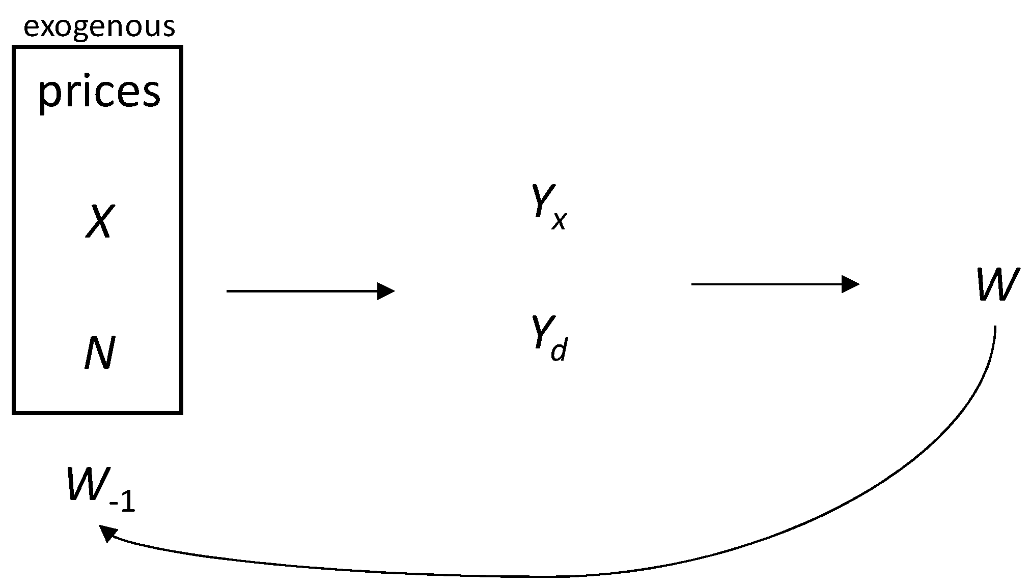
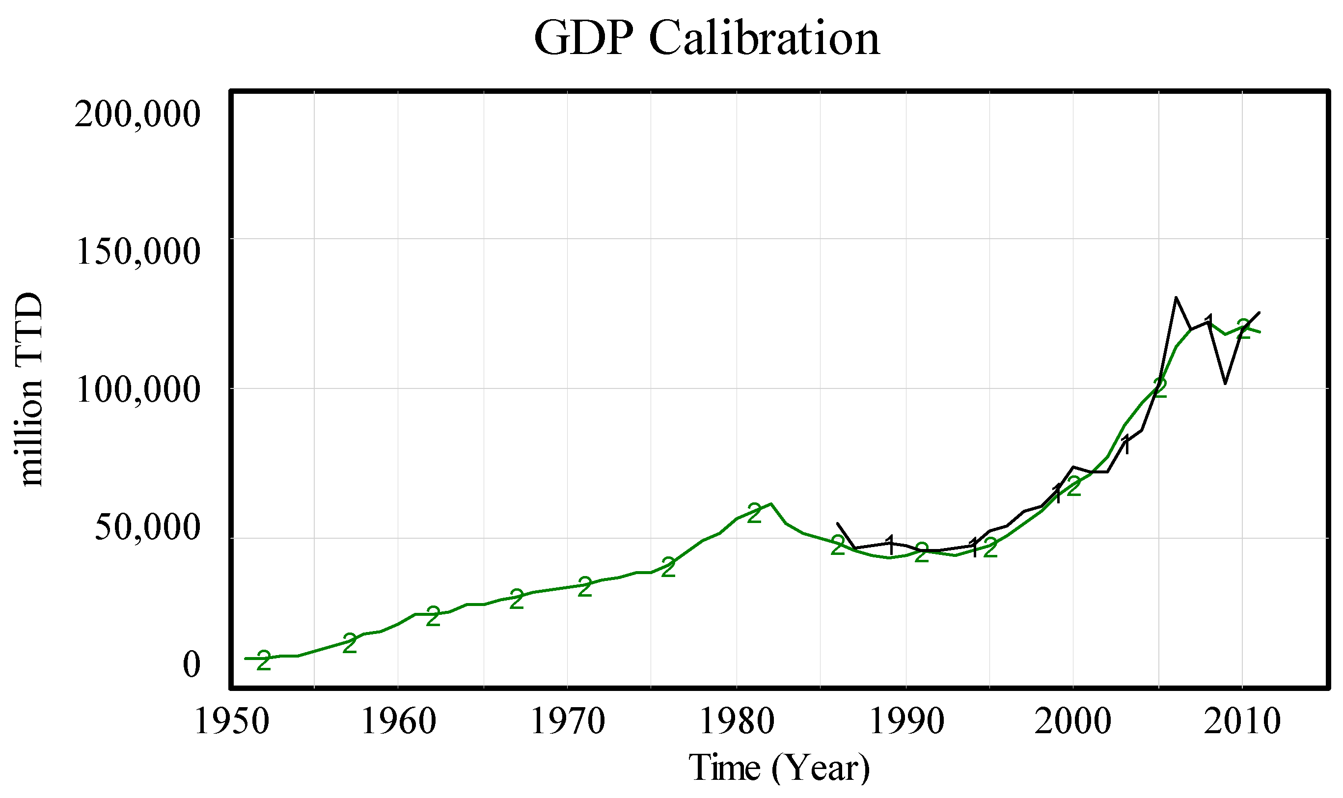
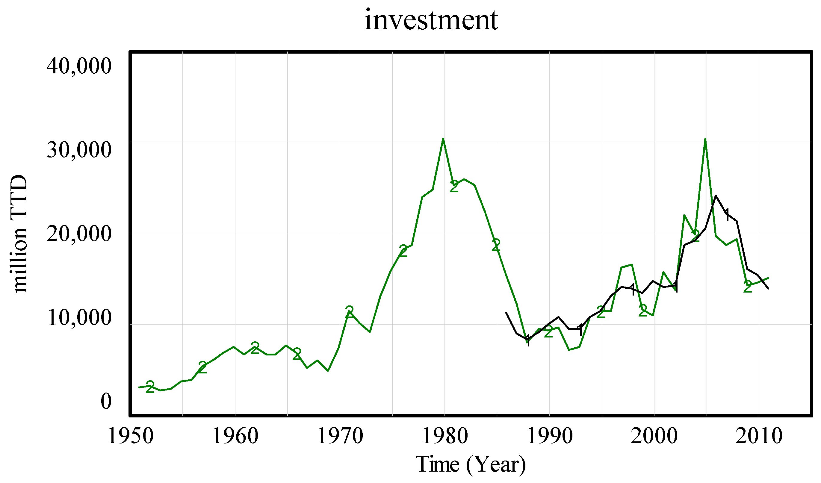
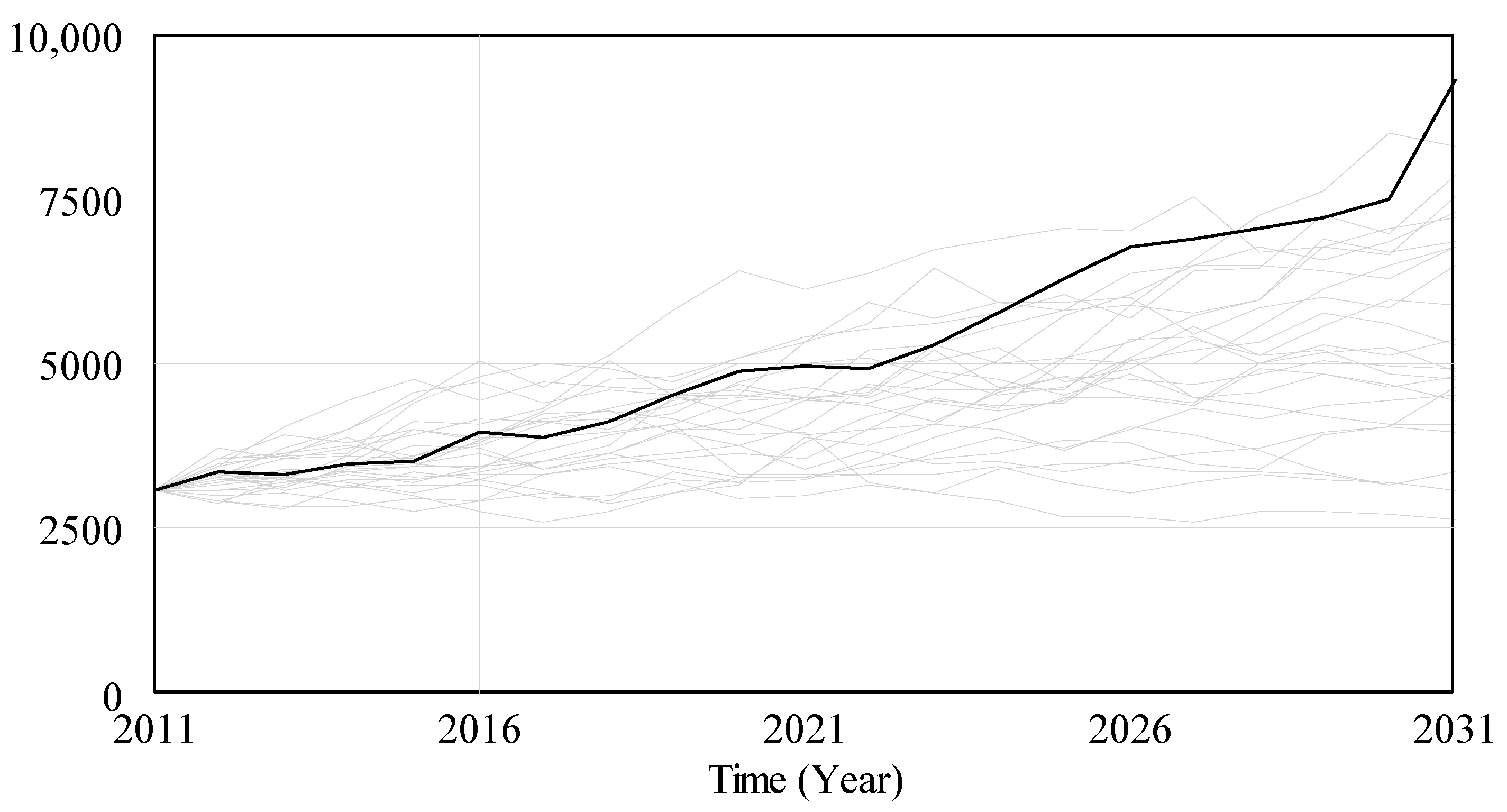
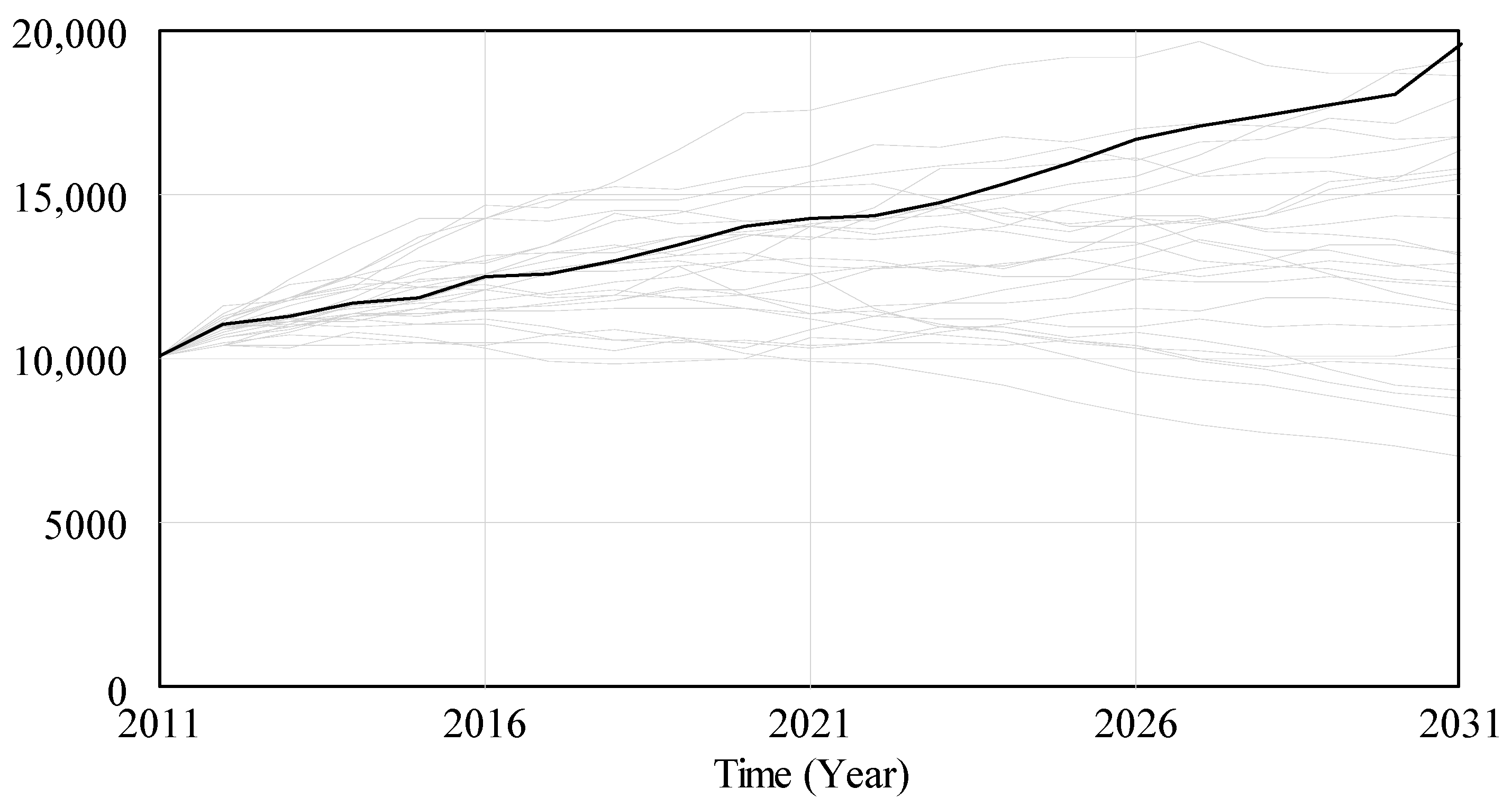
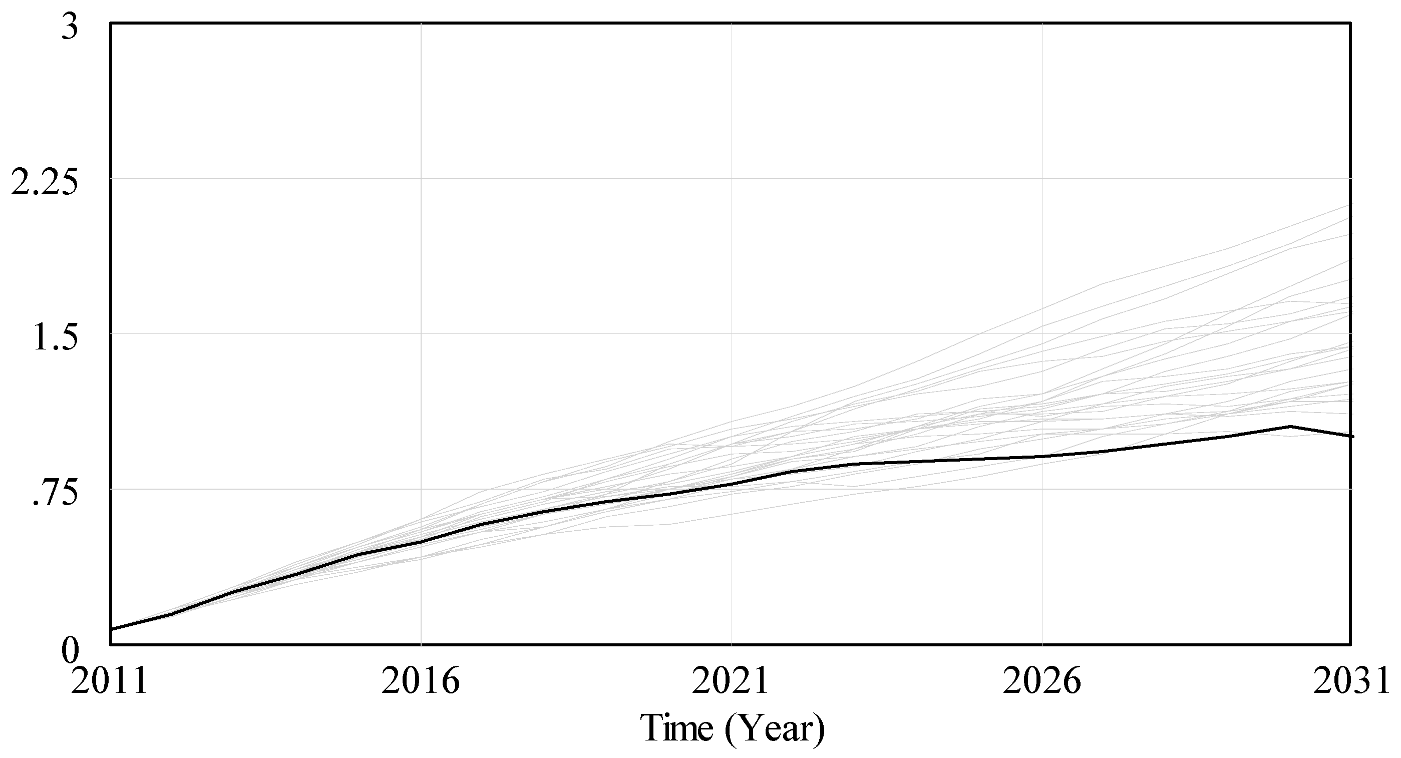
Table 1.
Goodness-of-fit statistics (underlined values indicate a potential problem).
| R2 | Adj R2 | DW | MAPE | Theil | |||
|---|---|---|---|---|---|---|---|
| Um | Uv | Uc | |||||
| Barbados | |||||||
| GDP | 0.85 | 0.76 | 0.45 | 3.1 | 0.06 | 0.03 | 0.91 |
| Investment | 0.79 | 0.70 | 1.03 | 8.9 | 0.00 | 0.08 | 0.92 |
| Imports | 0.94 | 0.93 | 1.77 | 4.4 | 0.00 | 0.27 | 0.73 |
| Jamaica | |||||||
| GDP | 0.85 | 0.76 | 0.85 | 3.9 | 0.20 | 0.00 | 0.80 |
| Investment | 0.92 | 0.89 | 1.07 | 4.8 | 0.00 | 0.04 | 0.96 |
| Debt | 0.93 | 0.92 | 1.26 | 10.7 | 0.00 | 0.21 | 0.78 |
| Imports | 0.69 | 0.64 | 0.69 | 8.2 | 0.00 | 0.35 | 0.64 |
| Trinidad and Tobago | |||||||
| GDP | 0.96 | 0.94 | 1.45 | 5.8 | 0.04 | 0.02 | 0.93 |
| Investment | 0.63 | 0.45 | 1.78 | 15.4 | 0.00 | 0.23 | 0.77 |
| Imports | 0.93 | 0.92 | 2.00 | 7.4 | 0.01 | 0.00 | 0.99 |
Table 2.
Estimated parameter values (underlined values are at the upper or lower end of the allowed range).
Table 2.
Estimated parameter values (underlined values are at the upper or lower end of the allowed range).
| Parameter | Barbados | Jamaica | Trinidad and Tobago |
|---|---|---|---|
| g0 | 0.017 | 0.046 | 0.040 |
| gu | 0.101 | 0.282 | 0.048 |
| gd | 0.017 | 0.013 | 0.001 |
| v* | 1.889 | 0.644 | 2.000 |
| m0 | 0.177 | 0.000 | 0.420 |
| εm | −0.123 | −2.802 | −3.000 |
| cx | 0.000 | 0.000 | 0.000 |
| sw | 0.000 | 0.034 | 0.468 |
| ωx | 0.400 | 0.372 | 0.400 |
| ωd | 0.700 | 0.700 | 0.699 |
| axd | 0.189 | 0.250 | 0.202 |
| adx | 0.250 | 0.500 | 0.250 |
| mx | 0.250 | 0.237 | 0.170 |
| md | 0.082 | 0.196 | 0.032 |
| i | 0.070 | 0.012 | 0.028 |
| ρK | 0.000 | 0.003 | pre-’97 0.081 post-’97 0.048 |
© 2018 by the authors. Licensee MDPI, Basel, Switzerland. This article is an open access article distributed under the terms and conditions of the Creative Commons Attribution (CC BY) license (http://creativecommons.org/licenses/by/4.0/).
Share and Cite
MDPI and ACS Style
Kemp-Benedict, E.; Drakes, C.; Laing, T.J. Export-Led Growth, Global Integration, and the External Balance of Small Island Developing States. Economies 2018, 6, 35. https://doi.org/10.3390/economies6020035
AMA Style
Kemp-Benedict E, Drakes C, Laing TJ. Export-Led Growth, Global Integration, and the External Balance of Small Island Developing States. Economies. 2018; 6(2):35. https://doi.org/10.3390/economies6020035
Chicago/Turabian StyleKemp-Benedict, Eric, Crystal Drakes, and Timothy J. Laing. 2018. "Export-Led Growth, Global Integration, and the External Balance of Small Island Developing States" Economies 6, no. 2: 35. https://doi.org/10.3390/economies6020035
Note that from the first issue of 2016, this journal uses article numbers instead of page numbers. See further details here.