Effect of Dangling Bonds on De-Poling Time for Polymeric Electric Field Optical Sensors

1
Applied-Science & Robotics Laboratory for Applied-Mechatronics (ARAtronics Lab.), Mechatronics Engineering Department, German University in Cairo, Cairo 11835, Egypt
2
Micro-Sensor Laboratory, Mechanical Engineering Department, Southern Methodist University, Dallas, TX 75275, USA
3
Faculty of Science (Girls), Chemistry Department, Al-Azhar University, Cairo 11675, Egypt
4
Faculty of Science (Boys), Chemistry Department, Al-Azhar University, Cairo 11675, Egypt
*
Author to whom correspondence should be addressed.
Chemosensors 2018, 6(1), 3; https://doi.org/10.3390/chemosensors6010003
Submission received: 26 November 2017
/
Revised: 10 January 2018
/
Accepted: 11 January 2018
/
Published: 12 January 2018
(This article belongs to the Special Issue Polymers Based Chemical Sensors)
Abstract
:This paper investigates the possible chemical changes in polydimethylsiloxane (PDMS) caused by two different techniques of fabrication for ultra-sensitive electric field optical sensors. The sensing element is a micro-sphere made from 60:1 PDMS (60 parts base silicon elastomer to one part polymer curing agent by volume). The measurement principle is based on the morphology dependent resonances (MDR) shifts of the micro-sphere. We present the effects of curing and poling of polymer micro-spheres used as optical sensors. The degree of curing leads to changes in the de-poling time which results from dangling bonds in the polymeric chains. Consequently, the longevity of the sensitivity of the sensor can extended by two orders of magnitude. An analysis is carried out along with preliminary experiments to investigate that behavior.
1. Introduction
In this paper, optical cavities depending on morphology-dependent resonances (MDR) will be used to sense the applied electric field. MDR are optical modes of dielectric cavities, such as toroids, spherical shells, and spheres. A tunable laser is used to excite such modes. The light is coupled tangentially from the laser into the sensing element using an optical fiber [1]. The optical modes are monitored as sharp dips in the transmission spectrum through the photodiode end of the fiber. These modes are also denoted as the morphology-dependent resonant MDR modes due to their high sensitivity to morphological variations (for example the dimension, shape, or refractive index) of the optical sensors. By monitoring the MDR shifts, these cavities can be used to accurately sense and measure various phenomena of the surrounding environment [2,3,4].
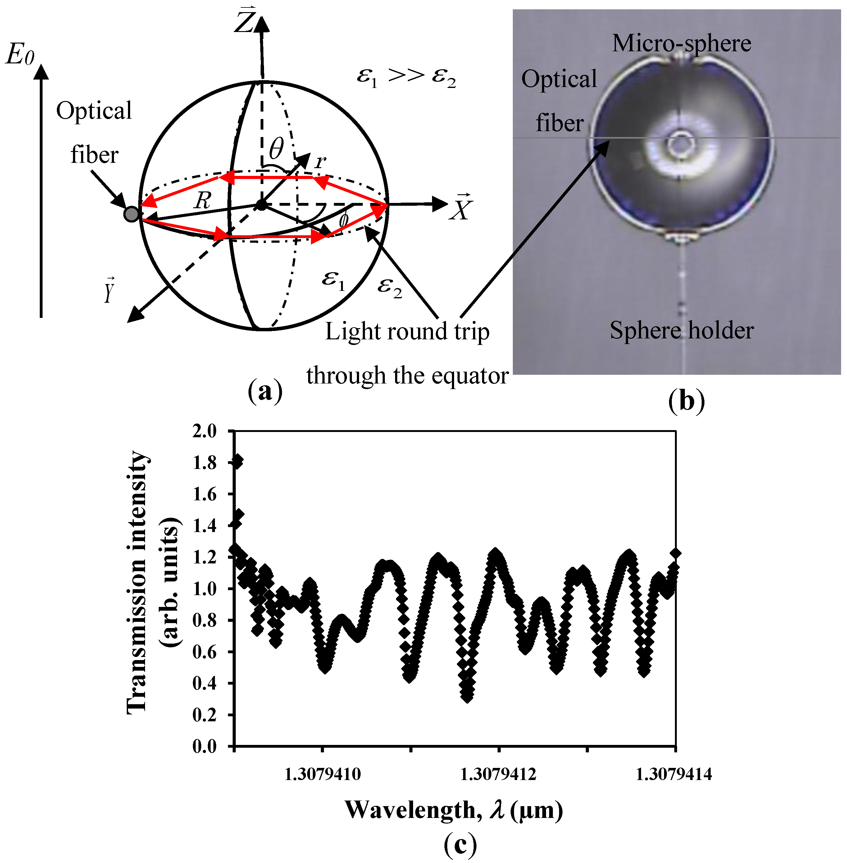
Geometric optics can easily describe the MDR phenomenon [5,6]. This description is legal at the first order approximation when the wavelength of the laser is much smaller compared to the size of the optical sensor. From the geometric point of view, light coupled at a grazing angle into a microsphere whose refractive index is larger than that of the surrounding medium circumnavigates through the interior surface of the sphere over the total internal reflection (as shown in Figure 1) and returns in phase. The condition for optical resonance is , where is the vacuum wavelength of the light (supplied by a laser), l is an integer, R is the sphere radius, and n0 is the sphere’s refractive index. When the sphere is subjected to the external electric field, its morphology changes (elastic deformation) due to the electrostriction effect. This, in turn, causes a perturbation of both the radius (ΔR) and refractive index (Δn), leading to a shift in the optical resonance (MDR), as follows:
The MDR is very sensitive to any change in its radius or index of refraction and, hence, can be tuned by causing a very small change in the measurand of the surrounding. Any small change in the surroundings can be measured by monitoring its MDR shifts due to the very high optical Q-factors that can exhibit the higher Q-factor indicates a lower rate of energy loss relative to the stored energy of the resonator [7,8].
Figure 1 shows the optical setup for the proposed sensor in the present paper. Once the light is coupled to the cavity through the tapered section in the optical fiber the MDR could be seen as sharp dips in the transmission spectrum, as seen in Figure 1c.
Recently, an MDR-based photonic electric field sensor was demonstrated [9,10,11,12,13]. The theory of operation is based on changing the radius of the cavity due to the electrostriction effect. The external electric field will perturb the sensor’s geometry leading to a shift in its MDR.
Electric field detections with high resolution may offer a more physiological means of neural modulation for prosthetic purposes than previously possible [14].
2. Experimental Investigation
2.1. Measurement Approach
The theory of operation depends on the morphology-induced shift of the optical sensors. In recent years, different applications used the proposed theory in sensing algorithms. The high quality factor, (where λ is the laser wavelength (~1.312 µm) and δλ is the resonance line width) is the main reason behind using the MDR micro-optical cavity in several applications. Q-factors can range from ca. 105 to 108, as reported in the literature [15]. Tangentially coupling the light to the cavity is one of the easiest methods to let the light start to interrogate through the total internal reflection of the cavity [12,16,17,18], as shown in Figure 1a. Recently, MDR micro-cavities have been used in applications including spectroscopy [19,20], micro-cavity laser technology [21], optical communications (switching [22], filtering [23], and multiplexing [24]), and sensor technologies [3,4,8,12,15,17,25,26,27,28,29,30,31,32,33]. In this paper, the electric field imposes a force on the dielectric microsphere (commonly referred to as the electrostriction effect) leading to the deformation of the sphere. The deformation is measured by tracking the MDR shifts of the sphere.
2.2. Experimental Opto-Electronics Setup
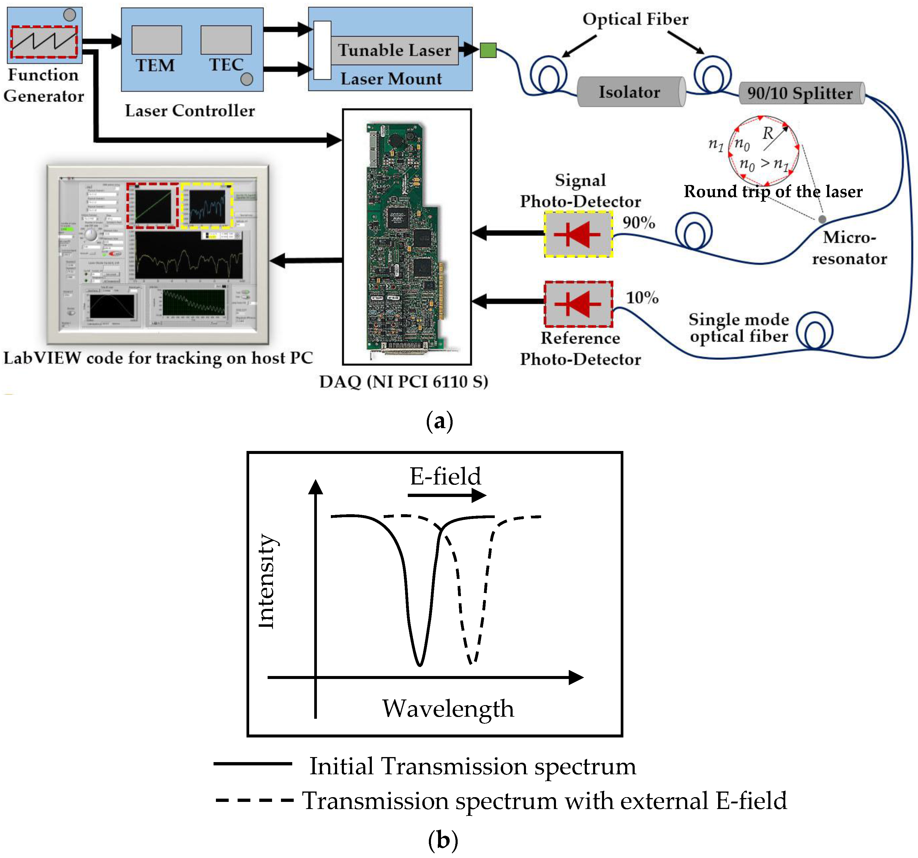
Figure 2 shows schematic for the interaction between the optical sensors and its signal processing. A single-mode optical fiber is used to obtain the output of a distributed feedback laser diode (DFB) with a nominal wavelength of ca. 1312 nm and power of 5 mW. A 90%:10% splitter is used to split the light intensity between the MDR sensor and the reference signal through the photo diode (PD), respectively. As is known, the wavelength of the light can be affected by temperature, so the laser controller is used to maintain the laser temperature constant during the measurements. Typically, a saw-tooth signal driven from the function generator is used to tune the light. All these gadgets will be sampled and monitored through a 16-bit data acquisition card (DAQ) and processed by a host personal computer (PC). By monitoring any shifts in the transmission spectrum of the resonance shifts in real-time, any perturbation around the cavity’s environment can be measured.
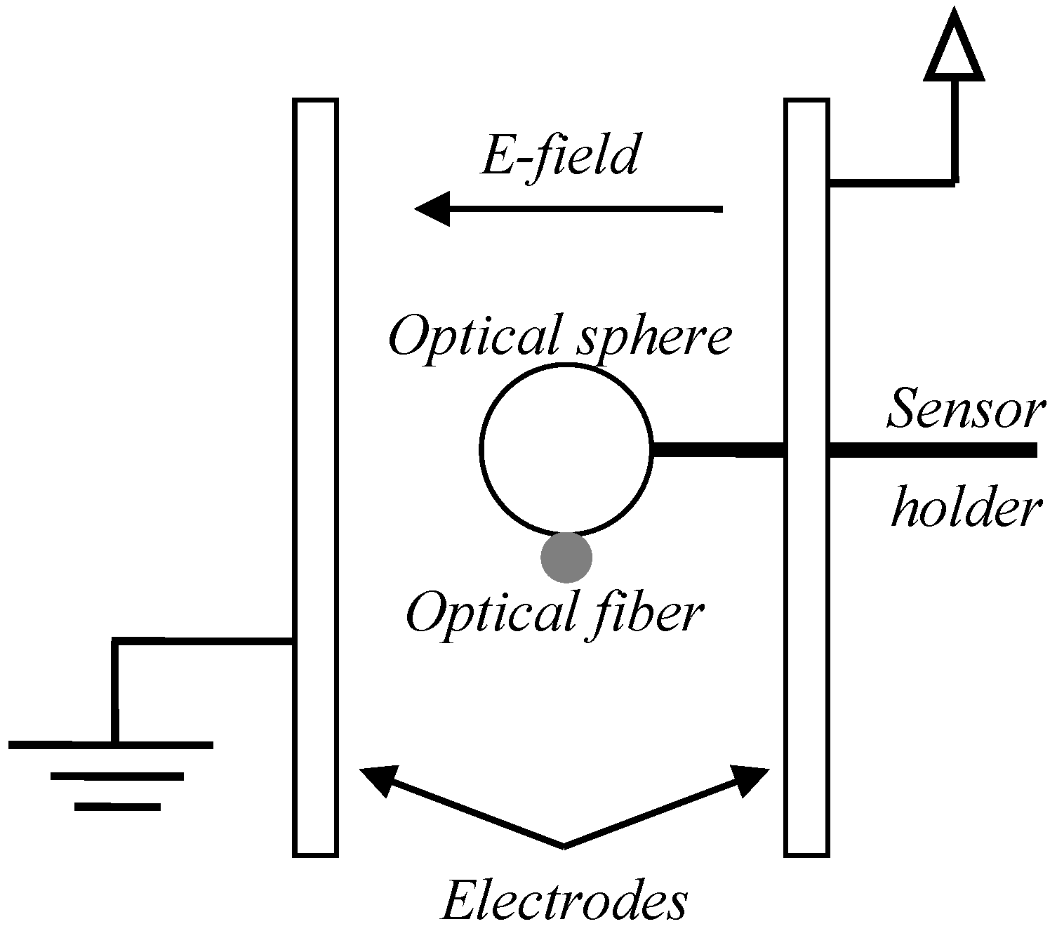
The external electric field will exert such a force on the polar direction of the cavity and compress it in the direction perpendicular to the optical fiber. Two electrodes made from brass are connected to a function generator in order to generate a harmonic electric field. Typically, the optical cavity would be laying between these two parallel electrodes as shown in Figure 3. Note that the polarization of an optical mode in the sphere is in a plane orthogonal to the light propagation and the observed resonances can be TE or TM modes. For large circumferential mode numbers (l = λ/2πRn0 >> 1, where R and n0 are the sphere radius and refractive index), the effect of mode polarization is negligible [11]. The optical Q-factor for the resonance shown in this paper is ca. 3 × 10⁵. Two different techniques are used to fabricate the sensing element; the first technique is called curing while poling (CWP) and the second one is called curing then poling (CTP).
2.3. Fabrication of Sensing Elements
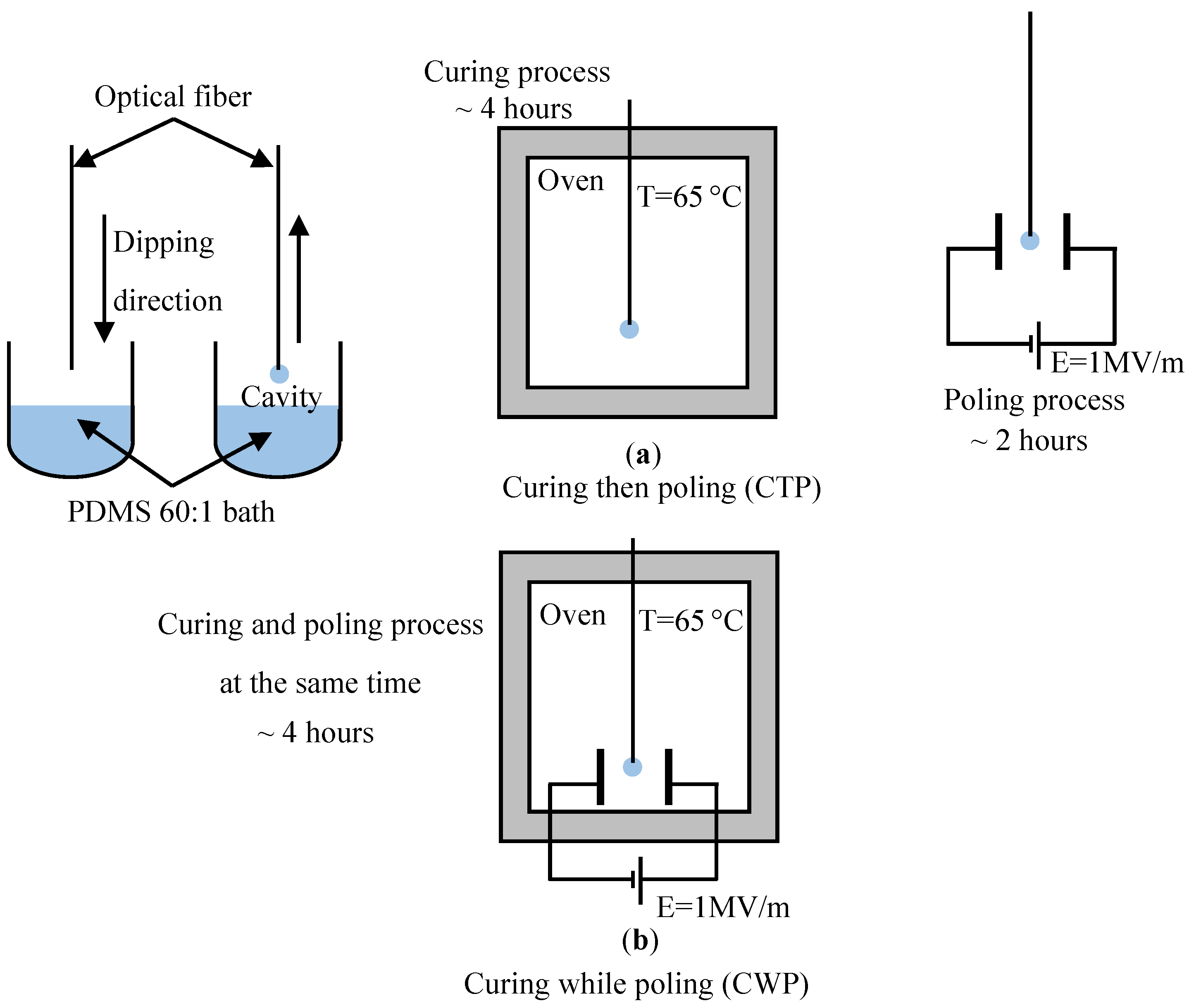
For both mentioned techniques (curing while poling and curing then poling) we using micro-optical cavities made from polymeric material. By dipping a piece of optical fiber in a bath of 60 parts of polydimethylsiloxane (PDMS) with one part polymer curing agent by volume, the cavities would be seen as spheres on top of these optical fibers. Due to the surface tension and the gravity the micro-optical cavities formed spherical shapes acting as an optical sensors. In order to get the light out of the optical fiber to become tangentially coupled with the micro-cavity and circumnavigate through the total internal reflection, the optical fiber should be heated using a micro torch and stretched at the same time to create a tapered section [34] in the middle part of the optical fiber with a ~10 to 20 μm in diameter. The sensor size kept close for both techniques CTP and CWP which is ca. 600 µm in diameter. In the first technique—curing then poling—typically we cure the 60:1 PDMS sensors in the oven for almost 4 h at 65 °C. After the sphere has been cured, it is poled for two hours in a uniform electric field of ca. 1 MV/m to develop surface charges so as to increase the electric field-induced force on it [16]. However, in the other technique—curing while poling—the sensor is cured at 65 °C and poled with ca. 1 MV/m at the same time, as seen in Figure 4, for almost 4 h. After we finished preparing the sensor for measurement, the electric field is generated by two brass plates connected to a function generator. The sphere is then placed between the electrodes (refer to Figure 3) and subjected to a harmonic external electric field by supplying voltage to the plates from the function generator. Then the comparison between both techniques using almost the same size of sensors (ca. 600 µm diameter) was performed and we kept all factors fixed, except the fabrication methods.
3. Experimental Results
Figure 5a shows the MDR shifts of the homogeneous sphere under a 0.2 Hz harmonic electric field perturbation with a 4 V/m amplitude. The corresponding sensitivity plot of the MDR shift vs. the electric field is presented in Figure 5b. The best fit of the data (solid line) indicates a sensitivity of Δλ/ΔE0 = 0.0197 pm/Vm−1. The corresponding electric field resolution is (ΔE0/Δλ) δλ ≈ 1.98 V/m. In this case, the standard deviation of the data scatter is δλ = 0.039 pm. Although the sensor becomes sufficiently sensitive in the electric field, it starts de-poling after a short period (within ca. 10 min) after poling, hence losing sensitivity, as shown in Figure 5c. This process for running the experiment in this way is called curing-then-poling (CTP). The other technique, using CWP, had the same behavior, sensitivity, and resolution because it is actually the same sensor, with the only difference between each being the de-poling time.
In this paper, we present a new method of sensor fabrication in order to mitigate this problem and to lock the polarization of the sensor’s material for a longer time with the same sensitivity. Another meethod to fabricate the sensing element should be used. The micro-sphere will be poled and cured simultaneously (curing-while-poling (CWP), refer to Figure 4b). When the previous experiment was repeated, but this time using the CWP method, we obtained almost the same sensitivity for the previous CTP technique, and the sensitivity for the sensing element starts to de-pole from ca. 0.0197 pm/Vm−1 to zero within ca. 6200 min. Chemical changes in the material of the sensing element caused by this new method of fabrication (CWP) enhanced the sensitivity period. The behavior of the dangling bonds for the partly cured PDMS leads to a two order of magnitude enhancement in the de-poling time, as shown in Figure 6. Additionally, it is clear that the magnitude of the poling affects the behavior of the sensing element under the same condition of the experiment. The higher poling magnitude will sustain the sensor’s sensitivity for a longer time, as seen in Figure 7. The sensitivity starts to de-pole within ca. 60 min when it is under a poling magnitude of up to 500 kV/m. However, the same sensing element has a longer de-poling time of ca. 6200 min when poled under 1 MV/m.
4. Analysis and Discussion
In this paper, a solid dielectric of radius, R, and inductive capacity was considered when it was subjected to a uniform electric field E0 in air, as shown in Figure 1a. The sphere is surrounded by a medium with inductive capacity . The external electric field exerts forces on the body of the sphere, fb, as well as forces on the sphere surface. The deformation of the sphere can be obtained by solving the Navier equation for a steady-state case:
where is the displacement vector of a given point within the sphere, and G are Poisson’s ratio and shear modulus of the sphere material, respectively. Electrostrictive body force induced by an external electric field is given by [9,13]:
where is the electric field within the sphere, is the dielectric constant, and a1 and a2 are coefficients that describe the electro-elastic properties of the sphere material. The parameters a1 and a2 represent the dependence of dielectric constant on mechanical strain in the directions parallel and normal to the electric field direction, respectively. The sphere rests on between the two electrodes as shown in Figure 7a and the electric field generated by connecting these two electrodes with a function generator.
In Figure 7b, the sphere could modeled as a linear spring with variable damper to be easily represented as a first order system as shown in the next equation:
where K, , , and are the static sensitivity, sensor’s time constant, variable damping coefficient, and the linear stiffness coefficient, respectively. Additionally, F(t) is the input force on the sphere in this case it could be the electrostrictive body force and γ(t) is the output deformation of the sphere.
When the micro-sphere poled and cured simultaneously curing-while-poling (CWP) or cured-then-poled (CTP) as seen in Figure 6, it seems that the sensitivity sooner or later needs to drop to the steady-state point (zero level). A situation like this is similar to first-order systems under step input. Then the solution for such a system is given by:
It is clear that when the time constant for the sensor, , is high; so the longer time will take to reach the steady-state point (zero level). On the other hand, the de-poling time which is represented by, td, will directly proportional with the time constant of the sensor, , where the time constant of the sensor is governed by the ratio of the damping coefficient to the stiffness coefficient for the sensor.
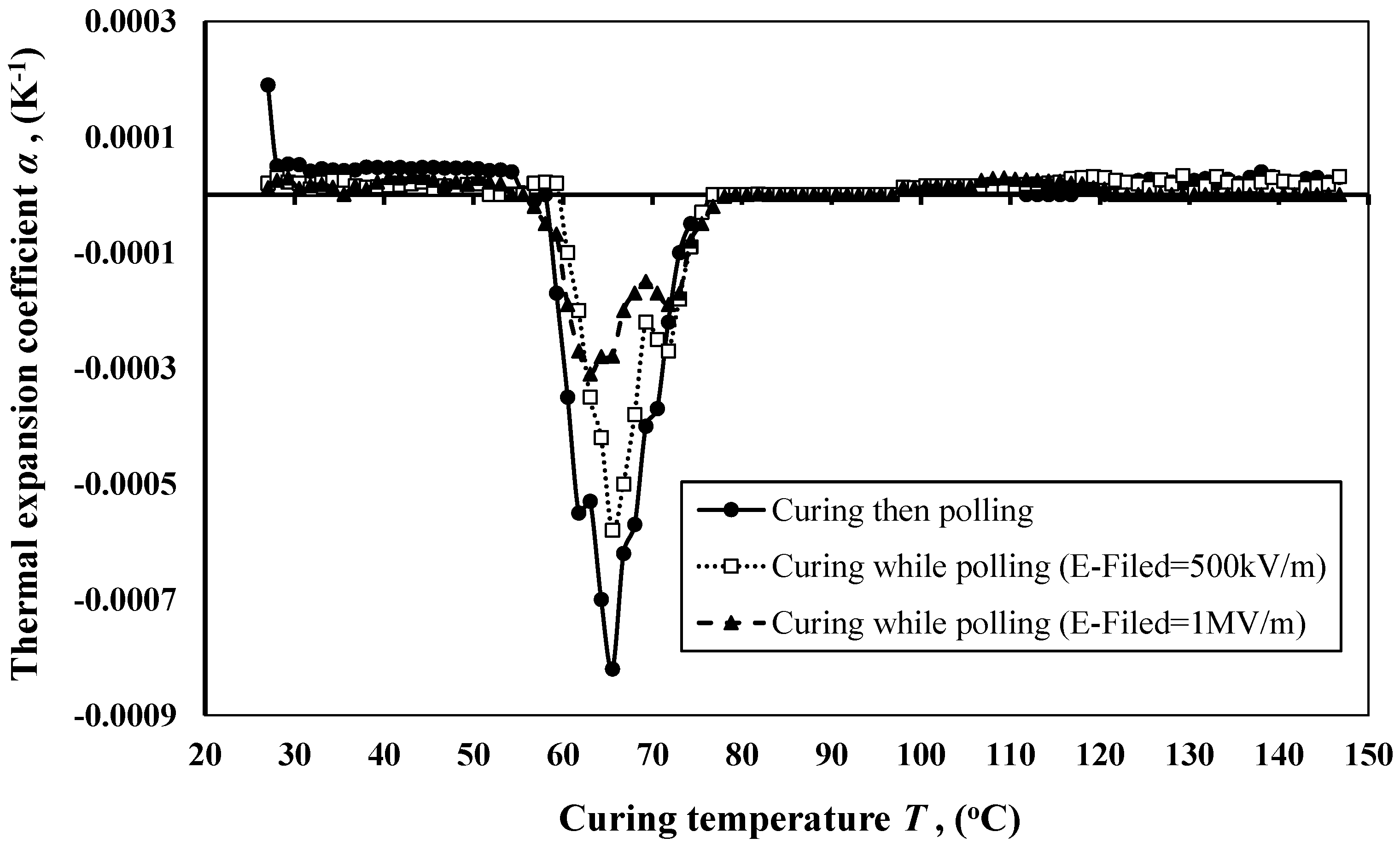
Since, this paper presents a new method of fabrication for the sensing elements called curing-while-poling (CWP) method versus the cured-then-poled (CTP), we created a polymeric sheet from the same mixtures that we made the sensors from. Then we test it using coefficient thermal expansion (CTE) determination. The application of the dependence of CTE on temperature method makes it possible to determine the geometrical dimension changes and the character structure changes. A CTE determination experiment was run on an electrical dilatometer. CTE determination was carried out for all CTP and CWP sensor fabrication methods.
In Figure 8 we can see that CTE obtains a negative value at T = 55–75 °C. This means that there are dangling bonds; therefore, the material is partly cured [35]. Sensors that cured without voltage have large quantities of dangling bonds, as well as areas of sharp energy absorption (jump) in the initial stage of cure continuation. For sensors cured in an electric field we can see this phenomenon in the final stage, which is evidence of polymer structural change.
A comparison among the thermal expansion coefficients in the case of CTP and CWP under 500 kV/m, and CWP under 1 MV/m were made. It becomes clear that the for CWP under 1 MV/m is higher than CWP under 500 kV/m, and is higher than CTP. Since there is expansion due to the temperature change caused by thermal strain, , and given by , by applying Hooke’s law we can relate the thermal strain, , to the modulus of elasticity (Es) as shown in Equation (6):
where and A are the normal stress due to thermal expansion and the cross-sectional area for the sensor. An inversely proportional relationship can be seen between the thermal expansion coefficient and the stiffness coefficient ks for the sensor, as revealed by Equation (6). Figure 8 proves that the CWP will increase the value for the thermal expansion coefficient and then decrease the stiffness coefficient of the sensors compared to the CTP. Thus, the time constant for the sensor, , will be enhanced significantly. In turn, the de-poling time for the sensor will be increased as well, and that matches with the experimental results shown in Figure 6.
5. Conclusions
An electric field optical sensor with long duration of sensitivity was demonstrated in this paper. The experiments were carried out by using two different fabrication techniques: cured-then-poled (CTP) and curing-while-poling (CWP). The coefficient thermal expansion (CTE) determination was analyzed for both fabrication techniques. The sensor fabricated by the (CTP process) showed a constant sensitivity of Δλ/ΔE0 = 0.0197 pm/Vm−1 and corresponding electric field resolution was (ΔE0/Δλ) δλ ≈ 1.98 V/m. Although the sensor does become sufficiently sensitive to electric fields, it starts de-poling after a short period (within ~10 min) after poling, hence losing sensitivity very quickly. On the other hand, the sensor fabricated by the new technique (CWP process) showed almost the same sensitivity, but starts de-poling after a long period (within ca. 6200 min). Just using this new fabrication technique enhanced the duration for the sensor sensitivity by two orders of magnitude. Due to the thermal expansion coefficient increased when we used the CWP compared to the CTP. In turn, the time constant for the sensor enhanced significantly by the same order. Thus, the de-poling time for the sensor increased, as well and that is exactly matching with the experimental results.
Author Contributions
The manuscript was written using the contributions of all authors. Amir R. Ali and Roushdy A. Ali designed the experiments; Amir R. Ali performed the experiments; Amir R. Ali, Amal S. Tourky and Roushdy A. Ali analyzed the data; and Amir R. Ali, Amal S. Tourky wrote the paper. All authors have given approval to the final version of the manuscript.
Conflicts of Interest
The authors declare no conflicts of interest.
References
- Serpengüzel, A.; Arnold, S.; Griffel, G. Excitation of resonances of microspheres on an optical fiber. Opt. Lett. 1995, 20, 654–656. [Google Scholar] [CrossRef] [PubMed]
- Rosenberger, A.T.; Rezac, J.P. Whispering-gallerymode evanescent-wave microsensor for trace-gas detection. Proc. SPIE 2001, 4265, 102–112. [Google Scholar]
- Das, N.; Ioppolo, T.; Ötügen, V. Investigation of a micro-optical concentration sensor concept based on whispering gallery mode resonators. In Proceedings of the 45th AIAA Aerospace Sciences Meeting and Exhibition, Reno, NV, USA, 8–11 January 2007. [Google Scholar]
- Guan, G.; Arnold, S.; Ötügen, M.V. Temperature Measurements Using a Micro-Optical Sensor Based on Whispering Gallery Modes. AIAA J. 2006, 44, 2385–2389. [Google Scholar] [CrossRef]
- Roll, G.; Schweiger, G. Geometrical optics model of Mie resonances. J. Opt. Soc. Am. A. 2000, 17, 1301–1311. [Google Scholar] [CrossRef]
- Roll, G.; Kaiser, T.; Lange, S.; Schweiger, G. Ray interpretation of multipole fields in spherical dielectric cavities. J. Opt. Soc. Am. A. 1998, 15, 2879–2891. [Google Scholar] [CrossRef]
- Gorodetsky, M.L.; Savchenkov, A.A.; Ilchenko, V.S. Ultimate Q of optical microsphere resonators. Opt. Lett. 1996, 21, 453–455. [Google Scholar] [CrossRef] [PubMed]
- Griffel, G.; Arnold, S.; Taskent, D.; Serpengüzel, A.; Connolly, J.; Morris, N. Morphology-dependent resonances of a microsphere–optical fiber system. Opt. Lett. 1996, 21, 695–697. [Google Scholar] [CrossRef] [PubMed]
- Ali, A.R.; Kamel, M.A. Mathematical model for electric field sensor based on whispering gallery modes using Navier’s equation for linear elasticity. J. Math. Probl. Eng. 2017, 2017, 9649524. [Google Scholar] [CrossRef]
- Ali, A.R.; Kamel, M.A. Novel techniques for optical sensor using single core multilayer structures for electric field detection. In Proceedings of the SPIE Optics & Optoelectronics, Prague, Czech Republic, 24–27 April 2017. [Google Scholar]
- Ali, A.R.; Ioppolo, T.; Ötügen, V.; Christensen, M.; MacFarlane, D. Photonic electric field sensor based on polymeric microspheres. J. Polym. Sci. Part B Polym. Phys. 2014, 52, 276–279. [Google Scholar] [CrossRef]
- Ioppolo, T.; Ötügen, M.V.; Ayaz, U.K. Development of whispering gallery mode polymeric micro-optical electric field sensors. J. Vis. Exp. 2013, e50199. [Google Scholar] [CrossRef] [PubMed]
- Ioppolo, T.; Stubblefield, J.; Ötügen, M.V. Electric field-induced deformation of polydimethylsiloxane polymers. J. Appl. Phys. 2012, 112, 044906. [Google Scholar] [CrossRef]
- Gluckman, B.J.; Nguyen, H.; Weinstein, S.L.; Schiff, S.J. Adaptive Electric Field Control of Epileptic Seizures. J. Neurosci. 2001, 21, 590–600. [Google Scholar] [CrossRef] [PubMed]
- Ioppolo, T.; Ayaz, U.K.; Ötügen, M.V. High-resolution force sensor based on morphology dependent optical resonances of polymeric spheres. J. Appl. Phys. 2009, 105, 013535. [Google Scholar] [CrossRef]
- Ali, A.R.; Ioppolo, T.; Ötügen, M.V. High-resolution electric field sensor based on whispering gallery modes of a beam-coupled dielectric resonator. In Proceedings of the 2012 International Conference on Engineering and Technology (ICET), Cairo, Egypt, 10–11 October 2012. [Google Scholar]
- Ayaz, U.; Ioppolo, T.; Ötügen, M.V. Wall shear stress sensor based on the optical resonances of dielectric microspheres. Meas. Sci. Technol. 2011, 22, 075203. [Google Scholar] [CrossRef]
- Serpengüzel, A.; Arnold, S.; Griffel, G.; Lock, J.A. Enhanced coupling to microsphere resonances with optical fibers. J. Opt. Soc. Am. B 1997, 14, 790–795. [Google Scholar] [CrossRef]
- Foreman, M.R. Single-particle Spectroscopy: Whispers of absorption. Nat. Photonics 2016, 10, 755–757. [Google Scholar] [CrossRef]
- Klitzing, W.V. Tunable whispering modes for spectroscopy and CQED Experiments. New J. Phys. 2001, 3, 14:1–14:14. [Google Scholar] [CrossRef]
- Cai, M.; Painter, O.; Vahala, K.J.; Sercel, P.C. Fiber-coupled microsphere laser. Opt. Lett. 2000, 25, 1430–1432. [Google Scholar] [CrossRef] [PubMed]
- Tapalian, H.C.; Laine, J.P.; Lane, P.A. Thermooptical switches using coated microsphere resonators. IEEE Photonics Technol. Lett. 2002, 14, 1118–1120. [Google Scholar] [CrossRef]
- Little, B.E.; Chu, S.T.; Haus, H.A.; Foresi, J.; Laine, J.P. Microring resonator channel dropping filters. J. Lightwave Technol. 1997, 15, 998–1005. [Google Scholar] [CrossRef]
- Offrein, B.J.; Germann, R.; Horst, F.; Salemink, H.W.M.; Beyerl, R.; Bona, G.L. Resonant coupler-based tunable add-after-drop filter in silicon-oxynitride technology for WDM networks. IEEE J. Sel. Top. Quantum Electron. 1999, 5, 1400–1406. [Google Scholar] [CrossRef]
- Ali, A.R.; Elias, C.M. Ultra-sensitive optical resonator for organic solvents detection based on whispering gallery modes. Chemosensors 2017, 5, 19. [Google Scholar] [CrossRef]
- Ali, A.R. Development of Whispering Gallery Mode Polymeric Micro-optical Sensors to Detect Chemical Impurities in Water Environment. Sci. Pages Photonics Opt. 2017, 1, 7–15. [Google Scholar]
- Ali, A.R.; Massoud, Y.M. Bio-optical sensor for brain activity measurement based on whispering gallery modes. In Proceedings of the SPIE Micro Technologies, Barcelona, Spain, 8–10 May 2017. [Google Scholar]
- Ali, A.R.; Afifi, A.N.; Taha, H. Optical signal processing and tracking of whispering gallery modes in real time for sensing applications. In Proceedings of the SPIE Micro Technologies, Barcelona, Spain, 8–10 May 2017. [Google Scholar]
- Ali, A.R.; Erian, A.; Shokry, K. Computational model and simulation for the whispering gallery modes inside micro-optical cavity. In Proceedings of the SPIE Micro Technologies, Barcelona, Spain, 8–10 May 2017. [Google Scholar]
- Ali, A.R.; Elias, C. Direct measurement for organic solvents diffusion using ultra-sensitive optical resonator. In Proceedings of the SPIE Micro Technologies, Barcelona, Spain, 8–10 May 2017. [Google Scholar]
- Ali, A.R.; Gatherer, A.; Ibrahim, M.S. Spinning optical resonator sensor for torsional vibrational applications measurements. In Proceedings of the SPIE LASE International Society for Optics and Photonics, San-Francisco, CA, USA, 22 April 2016. [Google Scholar]
- Matsko, A.B.; Savchenkov, A.A.; Strekalov, D.; Ilchenko, V.S.; Maleki, L. Review of application of whispring-gallery mode resonators in photonics and nonlinear optics. IPN Prog. Rep. 2005, 42–162, 1–51. [Google Scholar]
- Huston, A.L.; Eversole, J.D. Strain-sensitive elastic scattering from cylinders. Opt. Lett. 1993, 18, 1104–1106. [Google Scholar] [CrossRef] [PubMed]
- Knight, J.C.; Cheung, G.; Jacques, F.; Birks, T.A. Phase-matched excitation of whispering-gallery-mode resonances by a fiber taper. Opt. Lett. 1997, 22, 1129–1131. [Google Scholar] [CrossRef] [PubMed]
- Lemke, B.P.; Haneman, D. Dangling bonds on silicon. Phys. Rev. B 1978, 17, 1893. [Google Scholar] [CrossRef]
Figure 1.
Microsphere coupled with an optical fiber: (a) schematic; (b) photograph; and (c) typical transmission spectra trough the sphere-coupled fiber.
Figure 1.
Microsphere coupled with an optical fiber: (a) schematic; (b) photograph; and (c) typical transmission spectra trough the sphere-coupled fiber.

Figure 2.
Typical (a) schematic of the opto-electonic setup for the MDR sensor system; and (b) schematic transmission spectrum for a spherical resonator.
Figure 2.
Typical (a) schematic of the opto-electonic setup for the MDR sensor system; and (b) schematic transmission spectrum for a spherical resonator.

Figure 3.
Typical schematic for the experimental setup.

Figure 4.
Schematic for the typical preparation for the sensing element in: (a) the curing then poling technique (CTP); and (b) the curing while poling technique (CWP).
Figure 4.
Schematic for the typical preparation for the sensing element in: (a) the curing then poling technique (CTP); and (b) the curing while poling technique (CWP).

Figure 5.
(a) The time response for the homogeneous sphere under 0.2 Hz harmonic electric field perturbation with 4 V/m amplitude, where Δλ is the output and the E0 is the input to the sphere; (b) the calibration curve for the sensor shows the relationship between the output and the input with the slope of the best fit of the data Δλ/ΔE0 = 0.0197 pm/Vm−1 and shows that the standard deviation of the data scatter is δλ = 0.039 pm; and (c) the de-poling time (td) for the micro-sphere under harmonic field perturbation fabricated using the curing-then-poling (CTP) method.
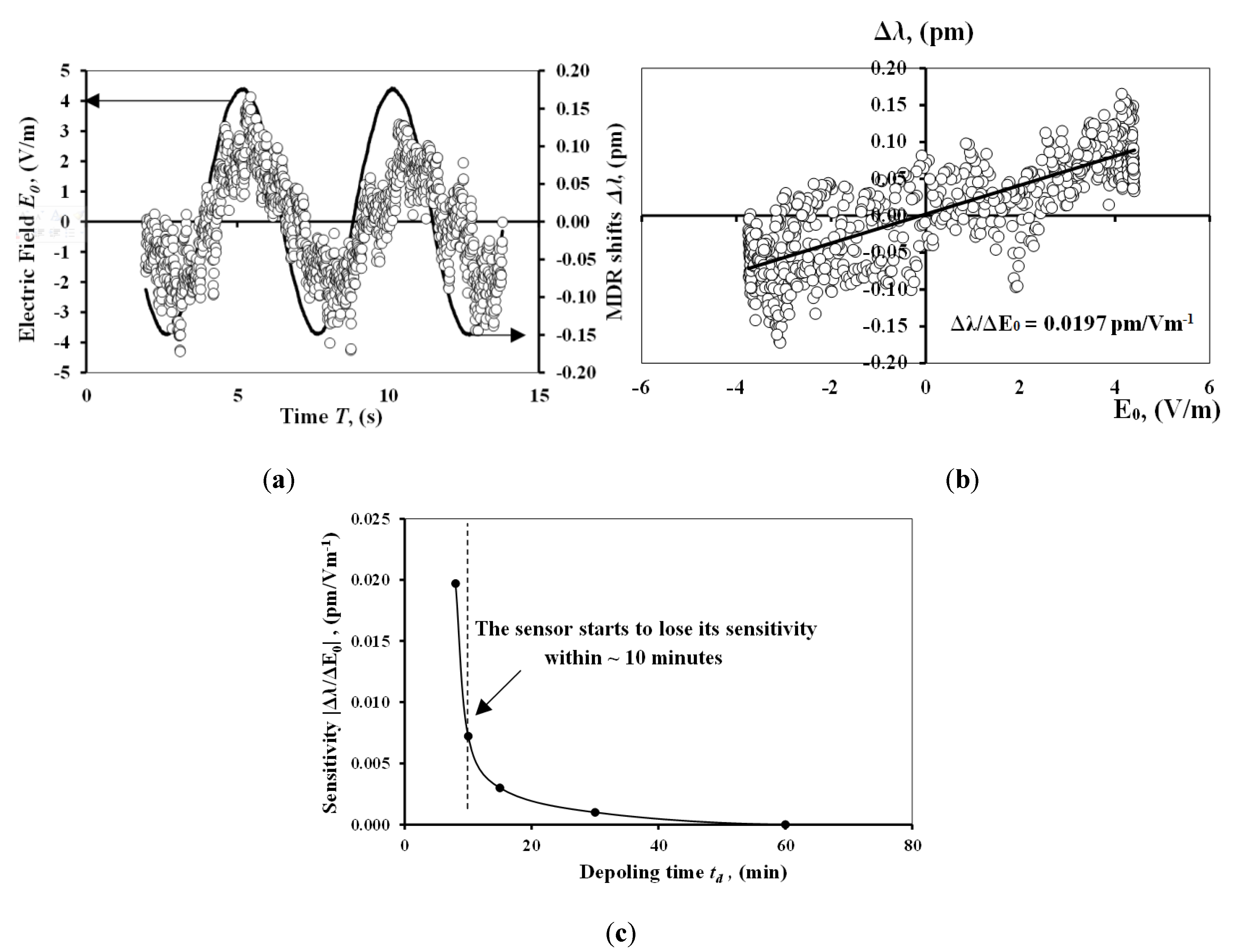
Figure 6.
De-poling time; for the micro-sphere under harmonic field perturbation fabricated using the curing-while-poling (CWP) method; where the ![Chemosensors 06 00003 i001]() is the curing then poling,
is the curing then poling, ![Chemosensors 06 00003 i002]() is the curing while poling in an electric field = 500 kV/m, and
is the curing while poling in an electric field = 500 kV/m, and ![Chemosensors 06 00003 i003]() is the curing while poling in an electric field = 1 MV/m.
is the curing while poling in an electric field = 1 MV/m.
 is the curing then poling,
  is the curing while poling in an electric field = 500 kV/m, and
  is the curing while poling in an electric field = 1 MV/m.
Figure 6.
De-poling time; for the micro-sphere under harmonic field perturbation fabricated using the curing-while-poling (CWP) method; where the ![Chemosensors 06 00003 i001]() is the curing then poling,
is the curing then poling, ![Chemosensors 06 00003 i002]() is the curing while poling in an electric field = 500 kV/m, and
is the curing while poling in an electric field = 500 kV/m, and ![Chemosensors 06 00003 i003]() is the curing while poling in an electric field = 1 MV/m.
is the curing while poling in an electric field = 1 MV/m.
is the curing then poling, is the curing while poling in an electric field = 500 kV/m, and is the curing while poling in an electric field = 1 MV/m.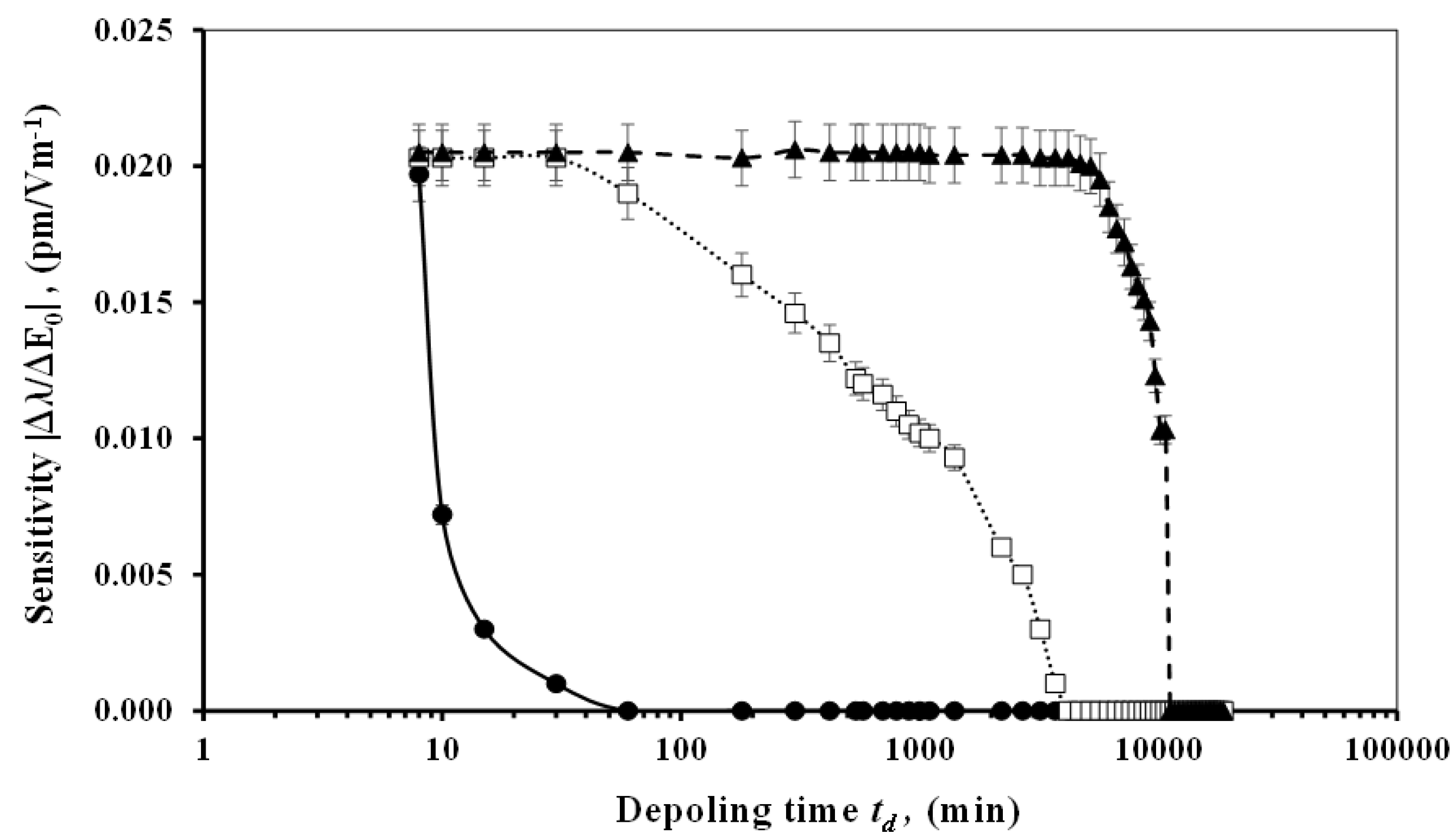
Figure 7.
Schematic for (a) the effect of the electric field on sphere morphology; and (b) the equivalent spring and damper representation for the sphere.
Figure 7.
Schematic for (a) the effect of the electric field on sphere morphology; and (b) the equivalent spring and damper representation for the sphere.
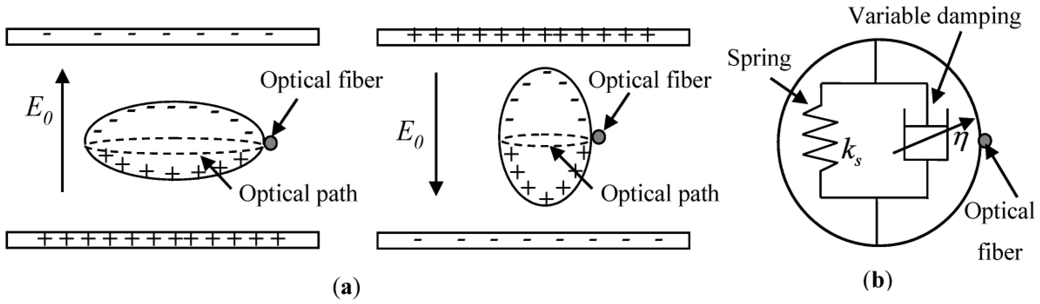
Figure 8.
Dependence of CTE on the CTP and CWP sensor fabrication methods.

© 2018 by the authors. Licensee MDPI, Basel, Switzerland. This article is an open access article distributed under the terms and conditions of the Creative Commons Attribution (CC BY) license (http://creativecommons.org/licenses/by/4.0/).
Share and Cite
MDPI and ACS Style
Ali, A.R.; Tourky, A.S.; Ali, R.A. Effect of Dangling Bonds on De-Poling Time for Polymeric Electric Field Optical Sensors. Chemosensors 2018, 6, 3. https://doi.org/10.3390/chemosensors6010003
AMA Style
Ali AR, Tourky AS, Ali RA. Effect of Dangling Bonds on De-Poling Time for Polymeric Electric Field Optical Sensors. Chemosensors. 2018; 6(1):3. https://doi.org/10.3390/chemosensors6010003
Chicago/Turabian StyleAli, Amir R., Amal S. Tourky, and Roushdy A. Ali. 2018. "Effect of Dangling Bonds on De-Poling Time for Polymeric Electric Field Optical Sensors" Chemosensors 6, no. 1: 3. https://doi.org/10.3390/chemosensors6010003
Note that from the first issue of 2016, this journal uses article numbers instead of page numbers. See further details here.