Optimal Deterministic Investment Strategies for Insurers

Abstract

We consider an insurance company whose risk reserve is given by a Brownian motion with drift and which is able to invest the money into a Black–Scholes financial market. As optimization criteria, we treat mean-variance problems, problems with other risk measures, exponential utility and the probability of ruin. Following recent research, we assume that investment strategies have to be deterministic. This leads to deterministic control problems, which are quite easy to solve. Moreover, it turns out that there are some interesting links between the optimal investment strategies of these problems. Finally, we also show that this approach works in the Lévy process framework.

1. Introduction

Inspired by [1], we first consider a mean-variance problem for an insurance company, where the investment strategy has to be deterministic or, in other words, pre-determined at time zero. Mathematically, the strategy has to be ${\mathbb{F}}_0$-measurable. We assume that the risk reserve is given by a Brownian motion with drift and allow investments into a Black–Scholes market with one bond and d risky assets. Investment strategies are determined by the amount of money that is invested in the assets. Such a model has been considered in [2] with one stock, but different optimization criteria, and in [3] with the emphasis towards time-consistency. Here, we present, first, the solution of the classical mean-variance problem, where we optimize over adapted wealth-dependent investment strategies. The solution procedure uses a standard Hamilton–Jacobi–Bellman (HJB) approach and follows along established lines, like in [4,5]. More interestingly, in the second part, we consider the same problem with deterministic investment strategies. The authors in [1] motivate this approach by remarking that such a kind of investment strategy is easier to implement, communicate and compare to alternatives. These kinds of strategies are also partly used in defined contribution pension plans. We refer the reader to [6], where, among others, the performance of deterministic and dynamic investment strategies is compared. In [1], the authors consider a mean-variance problem with additional consumption, and their investment strategies are given in terms of the fraction of wealth invested in the single risky asset. We would like to add that our deterministic investment strategies are mathematically easier to obtain and that there are some interesting and surprising links to optimal investment strategies for other optimization criteria, as we will explain below. Although, when we compare the densities for the final wealth, which are obtained under the optimal deterministic and dynamic investment strategies for the mean-variance problem, we will see that there is quite some difference.

Mathematically, the mean-variance problem for the restricted class of strategies leads to a deterministic control problem directly, without the problem of facing the non-separability of the target function. In the classical adapted case, it is necessary to link the mean-variance problem to an auxiliary linear-quadratic problem first (see, e.g., [5,7,8]) denoted by $QP(\eta )$ in Section 3. This step is not necessary in the deterministic case. Moreover, we will also show that in this special model with deterministic strategies, the mean-variance optimal strategy is also optimal for an arbitrary mean-risk problem, where the variance is replaced by an arbitrary law-invariant and positive homogeneous risk measure for the deviation of the terminal wealth from the mean. This is mainly due to the fact that the terminal wealth under a deterministic investment strategy has a normal distribution with mean and variance depending on the strategy. This observation can also be used to solve the control problem for other optimization criteria, like, e.g., expected exponential utility or the probability of ruin. Surprisingly, it will turn out that the classical optimal investment strategy for a company with exponential utility (within the class of adapted strategies) is deterministic and coincides with the optimal deterministic strategy for the mean-variance problem. Finally, we also show that this approach works when the involved processes are Lévy processes. In order to explain our procedure, we restrict the presentation to the most important case, where the risk reserve process is given as in the Cramér–Lundberg model, i.e., the risk reserve process is a compound Poisson process. Since the jumps vanish under expectation, we can proceed in almost the same way. In the classical setting with adapted strategies, it is also possible to deal with Lévy processes; see, e.g., [9,10] for LQ- and mean-variance problems, [11] for the exponential utility or [12] for more general information. In [13], a reinsurance problem with a Lévy market has been considered, and it turned out that the optimal reinsurance strategy is deterministic in the larger class of adapted strategies already. For a recent interesting comparison of different approaches to solve continuous-time mean-variance problems, see [14]. The authors there also consider non-negativity constraints on terminal wealth.

In this paper, we do not deal with questions of the time-consistency of the optimal investment strategy. This seems to be a key point in recent research. We just point to the recent papers [3,15,16], where time-consistency is discussed. The deterministic investment strategies depend on time only and are consistent for the deterministic control problem.

The paper is organized as follows: In the next section, we introduce the insurance model and the mean-variance problem along with some standing assumptions. Then, we explain how to reduce the problem in general to a stochastic linear-quadratic problem. Next, we solve the problem within the classical framework of adapted, i.e., wealth-dependent investment strategies. In Section 5, we consider the mean-variance problem with deterministic investment strategies. We show how the problem is turned into a deterministic control problem and solve it. In a special case, we study the form of the densities of the optimal terminal wealth for the mean-variance problem under deterministic and adapted investment strategies. The next section is dedicated to more general mean-risk problems and other optimization criteria. We show that for deterministic investment strategies, the optimal one is insensitive to the choice of the risk measure, as long as it is law-invariant and positive homogeneous. Finally, in the last section, we deal with the Lévy process framework. We assume that the risk reserve process follows a compound Poisson process, like in the Cramér–Lundberg model.

2. The Model

We suppose that the risk reserve process, $(Y_t)$, of the insurance company is given by the following stochastic differential equation:

$$d{Y}_t=\alpha dt+\beta d{\tilde{W}}_t$$

(1)

where $\tilde{W}=({\tilde{W}}_t)$ is a Brownian motion and $\alpha ,\beta$ are arbitrary real constants with $\beta \ge 0$, and it is reasonable, but not mathematically necessary to assume that $\alpha \ge 0$. The initial capital is given by $Y_0=x_0>0$. The risk reserve can be invested into a financial market, which is given by a riskless bond with price process $(S_0(t))$, where

$$S_0(t):=e^{rt}$$

and $r\ge 0$ denotes the deterministic interest rate. Further, there are d risky assets, and the price process $(S_i(t))$ of asset i is given by the stochastic differential equation:

$$d{S}_i(t)=S_i(t)\left(b_{i}dt+\sum _{j=1}^k{\sigma }_{ij}d{W}_j(t)\right)$$

with $S_i(0)=1$. The process $W=(W_t^1,\dots ,W_t^k)$ is a k-dimensional Brownian motion, which may be correlated with the driving Brownian motion of the risk reserve process. More precisely, we assume that ${\langle \tilde{W},W_j\rangle }_t={\rho }_{j}t$ for $j=1,\dots ,k$ and $\rho :={({\rho }_1,\dots ,{\rho }_k)}^{\top }$. In what follows, we set $b:={(b_1,\dots ,b_d)}^{\top }\in {\mathbb{R}}^d$ and $\sigma =({\sigma }_{ij})\in {\mathbb{R}}_{+}^{d\times k}$. We assume that all processes are defined on a common probability space $(\Omega ,\mathcal{F},\mathbb{P})$, that $({\mathbb{F}}_t)$ is the filtration generated by all Brownian motions and that there is a final time horizon $T>0$.

The insurance company is now allowed to invest the risk reserve into the financial market. A classical trading strategy $\pi =({\pi }_t)$ is an $({\mathbb{F}}_t)$-adapted stochastic process, where ${\pi }_t=({\pi }_1(t),\dots ,{\pi }_d(t))\in {\mathbb{R}}^d$ and ${\pi }_i(t)$ is the amount of money invested in stock i at time t. Note that short-selling is allowed and that the bond investment $({\pi }_0(t))$ is given by the self-financing condition. Adaptedness means that we assume that the decision maker is able to observe all Brownian motions, and, thus, the risk reserve and the evolution of the financial market, and is able to react to it. Given a trading strategy, π, and the notation $\mathfrak{1}:={(1,\cdots ,1)}^{\top }\in {\mathbb{R}}^d$, the corresponding wealth process of the insurance company follows the stochastic differential equation:

$$\begin{array}{ccc}\hfill d{X}_t^{\pi }& =& \left[r{X}_t^{\pi }+\alpha +{(b-r\mathfrak{1})}^{\top }{\pi }_t\right]dt+\beta d{\tilde{W}}_t+{\pi }_t^{\top }\sigma d{W}_t\hfill \end{array}$$

(2)

$$\begin{array}{ccc}\hfill X_0^{\pi }& =& x_0\hfill \end{array}$$

(3)

In what follows, let us denote $\Sigma :=\sigma {\sigma }^{\top }$, which we assume to be positive definite. Since the quadratic variation of $(X_t^{\pi })$ is given by:

$$d{\langle X^{\pi }\rangle }_t=\left[{\pi }_t^{\top }\Sigma {\pi }_t+{\beta }^2+2\beta {\pi }_t^{\top }\sigma \rho \right]dt$$

(4)

the process $(X_t^{\pi })$ is in a distribution equal to:

$$d{X}_t^{\pi }=\left[r{X}_t^{\pi }+\alpha +{(b-r\mathfrak{1})}^{\top }{\pi }_t\right]dt+\sqrt{{\pi }_t^{\top }\Sigma {\pi }_t+{\beta }^2+2\beta {\pi }_t^{\top }\sigma \rho }d{\widehat{W}}_t$$

(5)

for a generic Brownian motion, $\widehat{W}$. The generator of the controlled Markov process $(X_t^{\pi })$ is for $v\in C^{1,2}$ given by:

$${\mathcal{A}}^{\pi }v(t,x)=v_t+v_x\left(rx+\alpha +{(b-r\mathfrak{1})}^{\top }\pi \right)+\frac{1}{2}{v}_{xx}({\pi }^{\top }\Sigma \pi +{\beta }^2+2\beta {\pi }^{\top }\sigma \rho )$$

(6)

We call an investment strategy, π, admissible if all integrals in Equation (4) exist and ${\mathbb{E}}_{x_0}[{(X_T^{\pi })}^2]<\infty$. At first, we are interested in the dynamic mean-variance problem of the form (for $\mu \in \mathbb{R}$)

$$(MV)\left\{\begin{array}{c}{\mathrm{Var}}_{x_0}[X_T^{\pi }]\to min\hfill \\ {\mathbb{E}}_{x_0}[X_T^{\pi }]\ge \mu \hfill \\ \pi \mathrm{is\; an\; admissible\; investment\; strategy}\hfill \end{array}\right.$$

In the next section, we explain the standard way to transform this problem into a classical stochastic control problem, which will then be solved in the subsequent sections. In order to obtain non-trivial problems, we assume that:

$$\mu >x_0{e}^{rT}+(e^{rT}-1)\left(\frac{\alpha }{r}-\frac{\beta }{r}{(b-r\mathfrak{1})}^{\top }{\Sigma }^{-1}\sigma \rho \right)$$

(7)

We will discuss this condition later in a remark at the end of Section 5.

3. Transformation of MV to an Ordinary Stochastic Control Problem

Problem (MV) can be solved via the well-known Lagrange multiplier technique. The discussion in this section follows [17], chapter 4.6. Let $L_{x_0}(\pi ,\lambda )$ be the Lagrange-function, i.e.:

$$L_{x_0}(\pi ,\lambda ):={\mathrm{Var}}_{x_0}[X_T^{\pi }]+2\lambda \left(\mu -{\mathbb{E}}_{x_0}[X_T^{\pi }]\right)$$

for π is an admissible investment strategy and $\lambda \ge 0.$ As usual, $({\pi }^{*},{\lambda }^{*})$ with ${\lambda }^{*}\ge 0$ is called a saddle-point of the Lagrange-function, $L_{x_0}(\pi ,\lambda )$, if:

$$\underset{\lambda \ge 0}{sup}{L}_{x_0}({\pi }^{*},\lambda )=L_{x_0}({\pi }^{*},{\lambda }^{*})=\underset{\pi }{inf}{L}_{x_0}(\pi ,{\lambda }^{*})$$

Lemma 1 

Let $({\pi }^{*},{\lambda }^{*})$ be a saddle-point of $L_{x_0}(\pi ,\lambda ).$ Then, the value of (MV) is given by

$$\underset{\pi }{inf}\underset{\lambda \ge 0}{sup}{L}_{x_0}(\pi ,\lambda )=\underset{\lambda \ge 0}{sup}\underset{\pi }{inf}{L}_{x_0}(\pi ,\lambda )=L_{x_0}({\pi }^{*},{\lambda }^{*})$$

and ${\pi }^{*}$ is optimal for (MV).

Proof:

Obviously, the value of (MV) is equal to ${inf}_{\pi }{sup}_{\lambda \ge 0}{L}_{x_0}(\pi ,\lambda )$ and:

$$\underset{\pi }{inf}\underset{\lambda \ge 0}{sup}{L}_{x_0}(\pi ,\lambda )\ge \underset{\lambda \ge 0}{sup}\underset{\pi }{inf}{L}_{x_0}(\pi ,\lambda ).$$

For the reverse inequality, we obtain:

$$\begin{array}{ccc}\hfill \underset{\pi }{inf}\underset{\lambda \ge 0}{sup}{L}_{x_0}(\pi ,\lambda )& \le & \underset{\lambda \ge 0}{sup}{L}_{x_0}({\pi }^{*},\lambda )=L_{x_0}({\pi }^{*},{\lambda }^{*})\hfill \\ & =& \underset{\pi }{inf}{L}_{x_0}(\pi ,{\lambda }^{*})\le \underset{\lambda \ge 0}{sup}\underset{\pi }{inf}{L}_{x_0}(\pi ,\lambda )\hfill \end{array}$$

and the first statement follows. Further, from the definition of a saddle-point, we obtain for all $\lambda \ge 0$

$${\lambda }^{*}\left(\mu -{\mathbb{E}}_{x_0}[X_T^{{\pi }^{*}}]\right)\ge \lambda \left(\mu -{\mathbb{E}}_{x_0}[X_T^{{\pi }^{*}}]\right)$$

and, hence, ${\mathbb{E}}_{x_0}[X_T^{{\pi }^{*}}]\ge \mu$. Then, we conclude $L_{x_0}({\pi }^{*},{\lambda }^{*})={\mathrm{Var}}_{x_0}[X_T^{{\pi }^{*}}]$, and ${\pi }^{*}$ is optimal for (MV).☐

From Lemma 1, we see that it is sufficient to look for a saddle point $({\pi }^{*},{\lambda }^{*})$ of $L_{x_0}(\pi ,\lambda )$. It is not difficult to see that the pair $({\pi }^{*},{\lambda }^{*})$ is a saddle-point if ${\lambda }^{*}>0$ and ${\pi }^{*}={\pi }^{*}({\lambda }^{*})$ satisfy:

$${\pi }^{*}\mathrm{is\; optimal\; for}P({\lambda }^{*})and{\mathbb{E}}_{x_0}[X_T^{{\pi }^{*}}]=\mu$$

Here, $P(\lambda )$ denotes the so-called Lagrange-problem for the parameter $\lambda >0$

$$P(\lambda )\left\{\begin{array}{c}{L}_{x_0}(\pi ,\lambda )\to min\hfill \\ \pi \mathrm{is\; an\; admissible\; investment\; strategy}\hfill \end{array}\right.$$

Note that the problem $P(\lambda )$ is not a standard stochastic control problem. We embed the problem, $P(\lambda )$, into a tractable auxiliary problem, $QP(\eta )$, that turns out to be a stochastic LQ-problem. For $\eta \in \mathbb{R}$, define

$$QP(\eta )\left\{\begin{array}{c}{\mathbb{E}}_{x_0}\left[{(X_T^{\pi }-\eta )}^2\right]\to min\hfill \\ \pi \mathrm{is\; an\; admissible\; investment\; strategy}\hfill \end{array}\right.$$

The following result shows the relationship between the problems $P(\lambda )$ and $QP(\eta )$.

Lemma 2 

If ${\pi }^{*}$ is optimal for $P(\lambda )$, then ${\pi }^{*}$ is optimal for $QP(\eta )$ with $\eta :={\mathbb{E}}_{x_0}[X_T^{{\pi }^{*}}]+\lambda$.

Proof:

Suppose ${\pi }^{*}$ is not optimal for $QP(\eta )$ with $\eta :={\mathbb{E}}_{x_0}[X_T^{{\pi }^{*}}]+\lambda$. Then, there exists an admissible π, such that:

$${\mathbb{E}}_{x_0}[{(X_T^{\pi })}^2]-2\eta {\mathbb{E}}_{x_0}[X_T^{\pi }]<{\mathbb{E}}_{x_0}[{(X_T^{{\pi }^{*}})}^2]-2\eta {\mathbb{E}}_{x_0}[X_T^{{\pi }^{*}}]$$

Define the function $U:{\mathbb{R}}^2\to \mathbb{R}$ by

$$U(x,y):=y-x^2+2\lambda (\mu -x)$$

Then, U is concave and $U(x,y)=L_{x_0}(\pi ,\lambda )$ for $x:={\mathbb{E}}_{x_0}[X_T^{\pi }]$ and $y:={\mathbb{E}}_{x_0}[{(X_T^{\pi })}^2].$ Moreover, we set $x^{*}:={\mathbb{E}}_{x_0}[X_T^{{\pi }^{*}}]$ and $y^{*}:={\mathbb{E}}_{x_0}[{(X_T^{{\pi }^{*}})}^2].$ The concavity of U implies:

$$\begin{array}{ccc}\hfill U(x,y)& \le & U(x^{*},y^{*})-2(\lambda +x^{*})(x-x^{*})+y-y^{*}\hfill \\ & =& U(x^{*},y^{*})-2\eta (x-x^{*})+y-y^{*}<U(x^{*},y^{*})\hfill \end{array}$$

where the last inequality is due to our assumption $y-2\eta x<y^{*}-2\eta x^{*}.$ Hence, ${\pi }^{*}$ is not optimal for $P(\lambda )$, leading to a contradiction. ☐

The implication of Lemma 2 is that any optimal solution of $P(\lambda )$ (as long as it exists) can be found by solving problem $QP(\eta )$. Indeed, if $P(\lambda )$ has an optimal solution and if the optimal solution of $QP(\eta )$ is unique, it must be the optimal solution of $P(\lambda )$.

4. Solution of MV for a Classical Adapted Investor

We will first solve problem $QP(\eta )$, which is a classical stochastic control problem with no running cost and terminal cost ${(x-\eta )}^2$. Let us denote

$$V(t,x):=\underset{\pi }{inf}{\mathbb{E}}_{t,x}\left[{(X_T^{\pi }-\eta )}^2\right]$$

where, as usual, ${\mathbb{E}}_{t,x}$ is the conditional expectation given $X_t^{\pi }=x$. In view of the generator of the wealth process, the corresponding Hamilton–Jacobi–Bellman (HJB) equation reads (note that with a slight abuse of notation, we name the action again π):

$$\begin{array}{ccc}\hfill 0& =& \underset{\pi \in {\mathbb{R}}^d}{inf}\{v_t+v_x\left(rx+\alpha +{(b-r\mathfrak{1})}^{\top }\pi \right)+\frac{1}{2}{v}_{xx}\left({\pi }^{\top }\Sigma \pi +{\beta }^2+2\beta {\pi }^{\top }\sigma \rho )\right\}\hfill \end{array}$$

(8)

$$\begin{array}{ccc}\hfill {(x-\eta )}^2& =& v(T,x)\hfill \end{array}$$

(9)

where we denote by $v_t$ and $v_x$ the partial derivatives. Since this is a standard LQ-problem, a solution of the HJB equation can easily be found by using the Ansatz $v(t,x)=A(t)+B(t)x+C(t)x^2$. Plugging this form into the HJB equation yields:

$$\begin{array}{ccc}\hfill 0& =& \underset{\pi \in {\mathbb{R}}^d}{inf}\{\dot{A}(t)+\dot{B}(t)x+\dot{C}(t)x^2+\left(B(t)+2C(t)x\right)\left(rx+\alpha +{(b-r\mathfrak{1})}^{\top }\pi \right)\hfill \\ & & +C(t)\left({\pi }^{\top }\Sigma \pi +{\beta }^2+2\beta {\pi }^{\top }\sigma \rho )\right\}\hfill \end{array}$$

where $\dot{A}(t)$ denotes the derivative w.r.t. time. The minimum point of this equation is given by:

$${\pi }^{*}(t,x)=-{\Sigma }^{-1}(b-r\mathfrak{1})\left(\frac{B(t)}{2C(t)}+x\right)-\beta {\Sigma }^{-1}\sigma \rho$$

(10)

Inserting the minimum point into the HJB equation and collecting the terms without x, the terms with x and the terms with $x^2$ yields the following ordinary differential equations for $B(t)$, $C(t)$ and $A(t)$:

$$\begin{array}{ccc}\hfill \dot{C}(t)& =& -C(t)\left(2r-{(b-r\mathfrak{1})}^{\top }{\Sigma }^{-1}(b-r\mathfrak{1})\right)\hfill \end{array}$$

(11)

$$\begin{array}{ccc}\hfill \dot{B}(t)& =& -B(t)\left(r-{(b-r\mathfrak{1})}^{\top }{\Sigma }^{-1}(b-r\mathfrak{1})\right)-2C(t)\left(\alpha -\beta {(b-r\mathfrak{1})}^{\top }{\Sigma }^{-1}\sigma \rho \right)\hfill \end{array}$$

(12)

$$\begin{array}{ccc}\hfill \dot{A}(t)& =& -B(t)\left(\alpha -\beta {(b-r\mathfrak{1})}^{\top }{\Sigma }^{-1}\sigma \rho \right)-C(t){\beta }^2\left(1-{\rho }^{\top }{\sigma }^{\top }{\Sigma }^{-1}\sigma \rho \right)+\hfill \end{array}$$

(13)

$$\begin{array}{ccc}& & +{(b-r\mathfrak{1})}^{\top }{\Sigma }^{-1}(b-r\mathfrak{1})\frac{B{(t)}^2}{4C(t)}\hfill \end{array}$$

(14)

with boundary condition $C(T)=1,B(T)=-2\eta ,A(T)={\eta }^2$. The differential equation for $A(t)$ involves only $B(t)$ and $C(t)$ on the right-hand side. Since we are only interested in the optimal investment strategy, ${\pi }^{*}$, the interesting quantity is $h(t):=\frac{B(t)}{C(t)}$. For $h(t)$, we obtain the differential equation

$$\dot{h}(t)=\frac{\dot{B}(t)C(t)-B(t)\dot{C}(t)}{C^2(t)}=h(t)r-2\delta r$$

with $\delta r:=\alpha -\beta {(b-r\mathfrak{1})}^{\top }{\Sigma }^{-1}\sigma \rho$ and boundary condition $h(T)=-2\eta$. A solution is given by

$$h(t)=2\delta -2(\delta +\eta )e^{-r(T-t)}$$

Plugging this expression into Equation (10) yields:

$${\pi }^{*}(t,x)=-{\Sigma }^{-1}(b-r\mathfrak{1})\left(\delta -(\delta +\eta )e^{-r(T-t)}+x\right)-\beta {\Sigma }^{-1}\sigma \rho$$

(15)

Altogether, we obtain the following result with a standard verification argument (cf., for example, [4,18]):

Theorem 3 

The value function of problem $QP(\eta )$ is given by $V(t,x)=A(t)+B(t)x+C(t)x^2$ with $A,B,C$ being solutions of Equations (13), (12) and (11), respectively, and the optimal investment strategy $({\pi }_t^{*})$ is determined via Equation (15) by ${\pi }_t^{*}:={\pi }^{*}(t,X_t^{*})$, where $(X_t^{*})$ is the corresponding optimal wealth process solving Equation (5) with ${\pi }^{*}$.

Finally, we want to solve problem (MV). Thus, we have to compute ${\mathbb{E}}_{x_0}[X_T^{*}]$, the expected terminal wealth under the optimal strategy, ${\pi }^{*}$, for $QP(\eta )$. We obtain:

$$\begin{array}{ccc}\hfill {\mathbb{E}}_{x_0}[X_t^{*}]& =& x_0+{\int }_0^{t}r{\mathbb{E}}_{x_0}[X_s^{*}]+\alpha +{(b-r\mathfrak{1})}^{\top }\mathbb{E}[{\pi }_s^{*}]ds\hfill \\ & =& x_0+{\int }_0^{t}r{\mathbb{E}}_{x_0}[X_s^{*}]+\delta r-a\left(\delta -(\delta +\eta )e^{-r(T-s)}+{\mathbb{E}}_{x_0}[X_s^{*}]\right)ds\hfill \end{array}$$

with $a:={(b-r\mathfrak{1})}^{\top }{\Sigma }^{-1}(b-r\mathfrak{1})$. Thus, ${\mathbb{E}}_{x_0}[X_T^{*}]$ follows from solving the ordinary differential equation:

$$\begin{array}{ccc}\hfill \dot{h}(t)& =& h(t)(r-a)+\delta r-\delta a+a(\delta +\eta )e^{-r(T-t)}\hfill \\ \hfill h(0)& =& x_0\hfill \end{array}$$

and we get:

$${\mathbb{E}}_{x_0}[X_T^{*}]=x_0{e}^{-T(a-r)}-\delta e^{-Ta}(1-e^{rT})+\eta (1-e^{-Ta})$$

From ${\mathbb{E}}_{x_0}[X_T^{*}]=\mu$, and $\eta ={\lambda }^{*}+\mu$ we conclude:

$${\lambda }^{*}=\frac{e^{-Ta}}{1-e^{-Ta}}\left(\mu -x_0{e}^{Tr}-\delta (e^{rT}-1)\right)$$

(16)

which is positive, due to Equation (7). Hence, we obtain the following result:

Theorem 4 

The optimal investment strategy, ${\pi }^{*}$, for problem (MV) is determined by Equation (15) with $\eta =\mu +{\lambda }^{*}$ and ${\lambda }^{*}$ given by Equation (16).

5. MV Problem for an Investor with Deterministic Investment Strategies

In this section, we assume now that the investment strategy has to be pre-determined, i.e., that the process, π is ${\mathbb{F}}_0$-measurable, which means it is deterministic and only a function of time. Thus, the fund manager of the insurance company has to explain at $t=0$ the investment strategy for the time horizon $[0,T]$ without using further knowledge about the evolution of the processes. This seems at least sometimes to be more realistic than the adaptive strategy Equation (15). A similar situation has been considered in [1], where the authors motivate such a strategy by pension funds often being managed by time-dependent investment strategies only. Hence, we consider

$$(MVD)\left\{\begin{array}{c}{\mathrm{Var}}_{x_0}[X_T^{\pi }]\to min\hfill \\ {\mathbb{E}}_{x_0}[X_T^{\pi }]\ge \mu \hfill \\ \pi \mathrm{is\; a\; deterministic\; investment\; strategy}\hfill \end{array}\right.$$

This is now the same problem over a smaller class of investment strategies. We consider the first problem $PD(\lambda )$:

$$PD(\lambda )\left\{\begin{array}{c}{\mathrm{Var}}_{x_0}[X_T^{\pi }]+2\lambda \left(\mu -{\mathbb{E}}_{x_0}[X_T^{\pi }]\right)\to min\hfill \\ \pi \mathrm{is\; a\; deterministic\; investment\; strategy}\hfill \end{array}\right.$$

Here, it is not necessary to consider the artificial problem, $QP(\eta )$. $PD(\lambda )$ can be transformed into a deterministic control problem as follows. To this end, note that the stochastic differential Equation (5) for the wealth can easily be solved. When we denote by ${\tilde{X}}_t^{\pi }=\frac{X_t^{\pi }}{S_0(t)}$ the discounted wealth process, then we obtain:

$${\tilde{X}}_t^{\pi }=x_0+{\int }_0^t{e}^{-rs}\left(\alpha +{(b-r\mathfrak{1})}^{\top }{\pi }_s\right)ds+{\int }_0^t{e}^{-rs}\sqrt{{\pi }_s^{\top }\Sigma {\pi }_s+{\beta }^2+2\beta {\pi }_s^{\top }\sigma \rho }d{\widehat{W}}_s$$

(17)

For a deterministic process, π, the second integral is obviously a true martingale, and we obtain:

$$\begin{array}{ccc}\hfill {\mathbb{E}}_{x_0}[{\tilde{X}}_t^{\pi }]& =& x_0+{\int }_0^t{e}^{-rs}\left(\alpha +{(b-r\mathfrak{1})}^{\top }{\pi }_s\right)ds=:x(t)\hfill \\ \hfill {\mathrm{Var}}_{x_0}[{\tilde{X}}_t^{\pi }]& =& {\int }_0^t{e}^{-2rs}\left({\pi }_s^{\top }\Sigma {\pi }_s+{\beta }^2+2\beta {\pi }_s^{\top }\sigma \rho \right)ds=:y(t)\hfill \end{array}$$

Note that $x(t)$ and $y(t)$ both depend on π. Thus, the target function of $PD(\lambda )$ can be written as:

$$\begin{array}{ccc}\hfill {\mathrm{Var}}_{x_0}[X_T^{\pi }]+2\lambda \left(\mu -{\mathbb{E}}_{x_0}[X_T^{\pi }]\right)& =& e^{2rT}{\mathrm{Var}}_{x_0}[{\tilde{X}}_T^{\pi }]+2\lambda \left(\mu -e^{rT}{\mathbb{E}}_{x_0}[{\tilde{X}}_T^{\pi }]\right)\hfill \\ & =& e^{2rT}y(T)+2\lambda (\mu -e^{rT}x(T))\hfill \end{array}$$

The deterministic control problem is then:

$$PD(\lambda )\left\{\begin{array}{c}{e}^{2rT}y(T)+2\lambda (\mu -e^{rT}x(T))\to min\hfill \\ \dot{x}(t)=e^{-rt}\left(\alpha +{(b-r\mathfrak{1})}^{\top }{\pi }_t\right)\hfill \\ \dot{y}(t)=e^{-2rt}\left({\pi }_t^{\top }\Sigma {\pi }_t+{\beta }^2+2\beta {\pi }_t^{\top }\sigma \rho \right)\hfill \\ {\pi }_t\in {\mathbb{R}}^d\hfill \end{array}\right.$$

The value function of this problem is:

$$V(t,x,y):=\underset{\pi }{inf}\left\{e^{2rT}y(T)+2\lambda (\mu -e^{rT}x(T))\right\}$$

Obviously, the related HJB equation is:

$$\begin{array}{ccc}\hfill 0& =& \underset{\pi \in {\mathbb{R}}^d}{inf}\{v_t+v_x{e}^{-rt}\left(\alpha +{(b-r\mathfrak{1})}^{\top }\pi \right)+v_y{e}^{-2rt}\left({\pi }^{\top }\Sigma \pi +{\beta }^2+2\beta {\pi }^{\top }\sigma \rho )\right\}\hfill \end{array}$$

(18)

$$\begin{array}{ccc}\hfill v(T,x,y)& =& e^{2rT}y+2\lambda (\mu -e^{rT}x)\hfill \end{array}$$

(19)

In order to find a solution, we now consider the Ansatz

$$v(t,x,y)=e^{2rT}(y+g(t))+2\lambda \left(\mu -e^{rT}(x+f(t))\right)$$

with $f(T)=g(T)=0$. Thus, we obtain:

$$\begin{array}{ccc}\hfill v_t& =& e^{2rT}\dot{g}(t)-2\lambda e^{rT}\dot{f}(t)\hfill \\ \hfill v_x& =& -2\lambda e^{rT}\hfill \\ \hfill v_y& =& e^{2rT}\hfill \end{array}$$

The minimizer of Equation (18) is determined by:

$$\begin{array}{ccc}\hfill {\pi }_t^{*}& =& -{\Sigma }^{-1}(b-r\mathfrak{1})\frac{v_x}{v_y}\frac{e^{rt}}{2}-\beta {\Sigma }^{-1}\sigma \rho \hfill \end{array}$$

$$\begin{array}{ccc}& =& {\Sigma }^{-1}(b-r\mathfrak{1})\lambda e^{-r(T-t)}-\beta {\Sigma }^{-1}\sigma \rho \hfill \end{array}$$

(20)

Plugging this into the HJB Equation (18) yields:

$$\begin{array}{ccc}\hfill 0& =& e^{2rT}\dot{g}(t)-2\lambda e^{rT}\dot{f}(t)-2\lambda e^{rT}{\dot{x}}^{*}(t)+e^{2rT}{\dot{y}}^{*}(t).\hfill \end{array}$$

Note that this equation is satisfied when $\dot{f}(t)=-{\dot{x}}^{*}(t)$ and $\dot{g}(t)=-{\dot{y}}^{*}(t)$; thus:

$$\begin{array}{ccc}\hfill f(t)& =& {\int }_t^T{e}^{-rs}\left(\alpha +{(b-r\mathfrak{1})}^{\top }{\pi }_s^{*}\right)ds\hfill \end{array}$$

(21)

$$\begin{array}{ccc}\hfill g(t)& =& {\int }_t^T{e}^{-2rs}\left({({\pi }_s^{*})}^{\top }\Sigma {\pi }_s^{*}+{\beta }^2+2\beta {({\pi }_s^{*})}^{\top }\sigma \rho \right)ds\hfill \end{array}$$

(22)

Note that under the control ${\pi }^{*}$ and corresponding state trajectories $x^{*},y^{*}$, it holds that $x^{*}(t)+f(t)={\mathbb{E}}_{x_0}[{\tilde{X}}_T^{*}]$ and $y^{*}(t)+g(t)={\mathrm{Var}}_{x_0}[{\tilde{X}}_T^{*}]$ for all $t\in [0,T]$. We summarize our results in the following theorem. A verification is straightforward.

Theorem 5 

The value function of problem $PD(\lambda )$ is given by

$$V(t,x,y)=e^{2rT}(y+g(t))+2\lambda \left(\mu -e^{rT}(x+f(t))\right)$$

with $f,g$ being solutions of Equations (21) and (22), respectively. The optimal investment strategy $({\pi }_t^{*})$ is given by Equation (20).

Finally, we solve problem (MVD). First note that:

$${\mathbb{E}}_{x_0}[X_T^{*}]=e^{rT}{x}_0+\delta (e^{rT}-1)+a\lambda T$$

From ${\mathbb{E}}_{x_0}[X_T^{*}]=\mu$, we obtain:

$${\lambda }^{*}={(aT)}^{-1}\left(\mu -e^{rT}{x}_0-\delta (e^{rT}-1)\right)$$

(23)

which is positive, due to condition Equation (7). Thus, we obtain the following result:

Theorem 6 

The optimal investment strategy, ${\pi }^{*}$, for problem (MVD) is determined by Equation (20) with ${\lambda }^{*}$ given by Equation (23).

Remark: In this setting, it is also easy to determine the strategy with the minimum achievable variance. In case the financial market is not perfectly correlated with the risk reserve, this minimal variance is not zero. For an arbitrary deterministic investment strategy, we obtain:

$$\begin{array}{ccc}\hfill {\mathrm{Var}}_{x_0}[X_T^{\pi }]& =& e^{2rT}{\int }_0^T{e}^{-2rs}\left({\pi }_s^{\top }\Sigma {\pi }_s+{\beta }^2+2\beta {\pi }_s^{\top }\sigma \rho \right)ds\hfill \end{array}$$

Minimizing this expression in ${\pi }_s$ yields the minimum variance investment strategy: ${\widehat{\pi }}_t\equiv -\beta {\Sigma }^{-1}\sigma \rho$ with corresponding minimal variance

$${\mathrm{Var}}_{x_0}[{\widehat{X}}_T]=\frac{1}{2r}{\beta }^2(1-{\rho }^{\top }{\sigma }^{\top }{\Sigma }^{-1}\sigma \rho )(e^{2rT}-1)$$

and expectation:

$${\mathbb{E}}_{x_0}[{\widehat{X}}_T]=x_0{e}^{rT}+\delta (e^{rT}-1)$$

Thus, in case $\mu \le x_0{e}^{rT}+\delta (e^{rT}-1)$, problem (MVD) is trivial, because then, $\widehat{\pi }$ satisfies the constraint ${\mathbb{E}}_{x_0}[{\widehat{X}}_T]\ge \mu$ and yields the minimal possible variance. As a result, condition Equation (7) is reasonable.

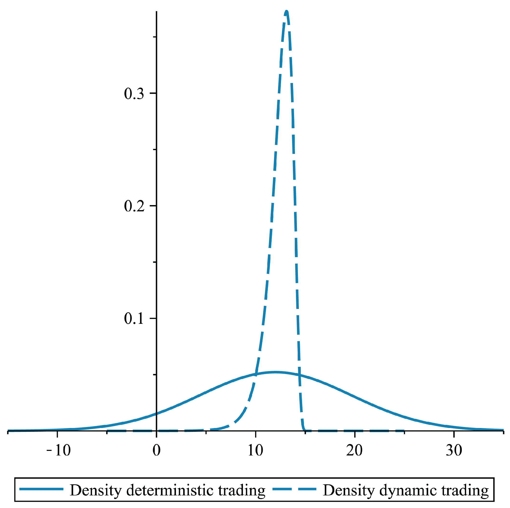
Remark: Of course, for a given expected return of μ, when we minimize the variance over the smaller set of deterministic investment strategies, the variance will be not smaller than in the classical stochastic case. Indeed, when we suppose that $\alpha =\beta =0$, i.e., no additional insurance business and $d=k=1$, we obtain the density of the optimal terminal wealth for (MVD), as well as for (MV). From Section 5, we conclude that for (MVD), the optimal terminal wealth satisfies:

$$X_T^{*}\sim N\left(\mu ,\frac{{(\mu -x_0{e}^{rT})}^2}{aT}\right)$$

For problem (MV), an optimal terminal wealth can be derived from the Lagrangian approach and is given by (cp.Theorem 3.3 in [14]):

$$X_T^{*}=\frac{1}{e^{aT}-1}\left(\mu e^{aT}-x_0{e}^{rT}+(x_0{e}^{rT}-\mu )L_T\right)$$

where $L_T$ is the risk neutral density given by:

$$L_T=exp\left(-\frac{1}{2}aT-\sqrt{a}{W}_T\right)$$

In Figure 1, we plotted the two densities of the optimal terminal wealth for (MVD) and (MV) for the parameters $x_0=10,\mu =12,r=0.02,b=0.15,\sigma =0.2$ and $T=1$.

Figure 1. Densities of the optimal terminal wealth for (MVD) and (MV).

Figure 1. Densities of the optimal terminal wealth for (MVD) and (MV).

Obviously, for this time horizon ($T=1$), there is a great difference in the performance of the two strategies. It seems that deterministic strategies here only make sense for small time horizons.

6. More General Mean-Risk Problems and Other Optimization Criteria

In this section, we will briefly discuss some other optimality criteria for the investment problem with deterministic investment strategies. Of course, when the solution of the classical stochastic control problem with adapted investment strategies yields an optimal strategy, which is itself deterministic, then this strategy is also optimal in the smaller class of deterministic strategies. A situation like this can occur when we consider the probability of ruin or the expected exponential utility as a target function. We discuss these cases below. However, we start this section with the observation that in the mean-variance framework, our optimal deterministic investment strategy is not only optimal w.r.t. to minimizing the variance.

6.1. More General Mean-Risk Problems

The variance or standard deviation is, of course, just one way to measure risk. Suppose now that ϱ is an arbitrary, law invariant and positive homogeneous risk measure, i.e., $\varrho (\lambda X)=\lambda \varrho (X)$ for all $\lambda >0$. We claim now that the problem

$$(MRD)\left\{\begin{array}{c}\varrho \left(X_T^{\pi }-{\mathbb{E}}_{x_0}[X_T^{\pi }]\right)\to min\hfill \\ {\mathbb{E}}_{x_0}[X_T^{\pi }]\ge \mu \hfill \\ \pi \mathrm{is\; a\; deterministic\; investment\; strategy}\hfill \end{array}\right.$$

has the same solution as (MVD), which is obtained when we use the standard deviation $\varrho (X):=\sqrt{\mathrm{Var}[X]}$.

Theorem 7 

The optimal investment strategy for (MRD) coincides with the optimal investment strategy for (MVD).

Proof:

First note that in both cases, because of ${\mathrm{Var}}_{x_0}[X_T^{\pi }]=e^{2rT}{\mathrm{Var}}_{x_0}[{\tilde{X}}_T^{\pi }]$ and the fact that $\varrho \left(X_T^{\pi }-{\mathbb{E}}_{x_0}[X_T^{\pi }]\right)=e^{rT}\varrho \left({\tilde{X}}_T^{\pi }-{\mathbb{E}}_{x_0}[{\tilde{X}}_T^{\pi }]\right)$, we can minimize the target function with $X_T^{\pi }$ replaced by ${\tilde{X}}_T^{\pi }$ and the side constraint, ${\mathbb{E}}_{x_0}[{\tilde{X}}_T^{\pi }]\ge \mu e^{-rT}.$ Now, due to Equation (17), we see that for deterministic investment strategies, ${\tilde{X}}_T^{\pi }$ has a normal distribution, $N(m_{\pi },s_{\pi }^2)$, with parameters:

$$\begin{array}{ccc}\hfill m_{\pi }& =& x_0+{\int }_0^T{e}^{-rs}\left(\alpha +{(b-r\mathfrak{1})}^{\top }{\pi }_s\right)ds\hfill \\ \hfill s_{\pi }^2& =& {\int }_0^T{e}^{-2rs}\left({\pi }_s^{\top }\Sigma {\pi }_s+{\beta }^2+2\beta \rho {\pi }_s^{\top }\sigma \right)ds\hfill \end{array}$$

Hence, in distribution $X_T^{\pi }\stackrel{d}{=}{m}_{\pi }+s_{\pi }Z$, where Z is a standard normal random variable. The optimization problem (MRD) can thus be written as:

$$(MRD)\left\{\begin{array}{c}\varrho (s_{\pi }Z)\to min\hfill \\ m_{\pi }\ge \mu e^{-rT}\hfill \\ \pi \mathrm{is\; a\; deterministic\; investment\; strategy}\hfill \end{array}\right.$$

Since ϱ is positive homogeneous, we obtain $\varrho (s_{\pi }Z)=s_{\pi }\varrho (Z)$, which means that we have to minimize the standard deviation of $X_T^{\pi }$. Hence, the statement follows. ☐

As a consequence, the optimal investment strategy we obtained is very robust w.r.t. the choice of risk measure. Indeed, it does not depend on the precise risk measure, as long as we agree to take a law invariant and positive homogeneous one. Indeed, the result is also valid for a function, ϱ, which is positive homogeneous of any order.

6.2. Maximizing Exponential Utility of Terminal Wealth

In this subsection, we consider the problem of maximizing ${\mathbb{E}}_{x_0}\left[-\frac{1}{\gamma }{e}^{-\gamma X_T^{\pi }}\right]$ with $\gamma >0$. For the classical stochastic case and only one stock, this has been done in [2]. We now directly consider the multi-asset model in the framework of deterministic strategies, i.e., we consider:

$$\left\{\begin{array}{c}{\mathbb{E}}_{x_0}[-\frac{1}{\gamma }{e}^{-\gamma X_T^{\pi }}]\to max\hfill \\ \pi \mathrm{is\; a\; deterministic\; investment\; strategy}\hfill \end{array}\right.$$

It turns out that the solution of this problem is very easy. We know already for deterministic π that $X_T^{\pi }$ has a normal distribution $N(m_{\pi },s_{\pi }^2)$ with parameters:

$$\begin{array}{ccc}\hfill m_{\pi }& =& e^{rT}\left(x_0+{\int }_0^T{e}^{-rs}\left(\alpha +{(b-r\mathfrak{1})}^{\top }{\pi }_s\right)ds\right)\hfill \\ \hfill s_{\pi }^2& =& e^{2rT}\left({\int }_0^T{e}^{-2rs}\left({\pi }_s^{\top }\Sigma {\pi }_s+{\beta }^2+2\beta \rho {\pi }_s^{\top }\sigma \right)ds\right)\hfill \end{array}$$

Hence, we can write $X_T^{\pi }=m_{\pi }+s_{\pi }Z$, and the target function thus reduces to:

$${\mathbb{E}}_{x_0}[-\frac{1}{\gamma }{e}^{-\gamma X_T^{\pi }}]=-\frac{1}{\gamma }{e}^{-\gamma m_{\pi }}{\mathbb{E}}_{x_0}[e^{-\gamma s_{\pi }Z}]=-\frac{1}{\gamma }{e}^{-\gamma m_{\pi }+\frac{1}{2}{\gamma }^2{s}_{\pi }^2}$$

Obviously, the problem is equivalent to minimizing $-\frac{2}{\gamma }{m}_{\pi }+s_{\pi }^2$, and we end up with the following deterministic control problem:

$$\left\{\begin{array}{c}{e}^{2rT}y(T)-\frac{2}{\gamma }{e}^{rT}x(T)\to min\hfill \\ \dot{x}(t)=e^{-rt}\left(\alpha +{(b-r\mathfrak{1})}^{\top }{\pi }_t\right)\hfill \\ \dot{y}(t)=e^{-2rt}\left({\pi }_t^{\top }\Sigma {\pi }_t+{\beta }^2+2\beta {\pi }_t^{\top }\sigma \rho \right)\hfill \\ {\pi }_t\in {\mathbb{R}}^d\hfill \end{array}\right.$$

However, this is equivalent to problem $PD(\lambda )$ with $\lambda =\frac{1}{\gamma }$, and we know from Equation (20) that the optimal investment strategy is given by:

$${\pi }_t^{*}={\Sigma }^{-1}(b-r\mathfrak{1})\frac{1}{\gamma }{e}^{-r(T-t)}-\beta {\Sigma }^{-1}\sigma \rho$$

Thus, due to Equation (23), there is a one-to-one relation between optimal mean-variance strategies and optimal strategies for the problem with the exponential utility function. For an early discussion about the relation of expected utility and mean-variance, see, e.g., [19,20]. Note that it can be shown that the optimal investment strategy we have computed here is also optimal within the larger class of adapted strategies.

6.3. Minimizing the Probability of Ruin

Another popular ‘risk measure’ in the actuarial sciences is the probability of ruin of a controlled risk reserve. When we consider the classical situation of $({\mathbb{F}}_t)$-adapted investment strategies, it is very easy to find the one which minimizes the probability of ruin of process Equation (5). According to [21], the optimal feedback function, ${\pi }^{*}(x)$, is obtained by maximizing the ratio of mean over variance of the process, i.e.:

$$\frac{rx+\alpha +{(b-r\mathfrak{1})}^{\top }\pi }{{\pi }^{\top }\Sigma \pi +{\beta }^2+2\beta {\pi }^{\top }\sigma \rho }$$

Obviously, when $r=0$, then the maximizer, ${\pi }^{*}$, is independent of x and deterministic. If further $d=k=1$ and $\alpha =0$, then ${\pi }^{*}=\frac{\beta }{\sigma }$.

7. Problems with Lévy Processes

The standard model for the risk reserve process of an insurance company is the so-called Cramér–Lundberg model. It assumes that the risk reserve process follows a Lévy process given as the difference of the premium income process and the claims that have been paid out so far. More precisely, it is usually assumed that:

$$Y_t=x_0+ct-\sum _{k=1}^{N_t}{U}_k$$

(24)

where $c>0$ is the premium income rate, $N=(N_t)$ is a Poisson process with parameter $\nu >0$, which counts the number of claims, and $U_1,U_2,\dots$ are independent and identically distributed random variables, representing the claim sizes. We denote $m:=\mathbb{E}U$ and $m_2:=\mathbb{E}{U}^2$. The process in Equation (1) can be seen as a diffusion approximation of process Equation (24) when claims are small and frequent. The mean-variance problems we have considered in Section 4 and Section 5 can be dealt with in a Lévy framework along the same lines. The solution of the classical problem (MV) may be derived from [10]. Here, we concentrate on the problem (MVD) with deterministic investment strategies. We assume that:

$$\mu >x_0{e}^{rT}+(e^{rT}-1)\frac{c-\nu m}{r}$$

(25)

In order to have an elegant notation, we write $(Y_t)$ with the help of its Poisson random measure, $M([0,t]\times B),t\ge 0,B\in \mathcal{B}({\mathbb{R}}_{+})$, which is the sum of all claims taking values in the set B up to time t. Hence, we can write:

$$Y_t=x_0+ct-{\int }_{[0,t]}{\int }_{{\mathbb{R}}_{+}}yM(ds,dy)$$

(26)

For simplicity, we leave the financial market as in the sections before, though one might also allow for jumps there. We again assume here that admissible trading strategies $\pi =({\pi }_t)$ are ${\mathbb{F}}_0$-measurable. The corresponding wealth of the insurance company follows the stochastic differential equation:

$$\begin{array}{ccc}\hfill d{X}_t^{\pi }& =& \left[r{X}_t^{\pi }+{(b-r\mathfrak{1})}^{\top }{\pi }_t\right]dt+d{Y}_t+{\pi }_t^{\top }\sigma d{W}_t\hfill \end{array}$$

(27)

$$\begin{array}{ccc}\hfill X_0^{\pi }& =& x_0\hfill \end{array}$$

We consider again the deterministic mean-variance problem (MVD) of Section 5. As in Section 5, we start with problem $PD(\lambda )$: Next, we compute ${\mathbb{E}}_{x_0}[X_t^{\pi }]$. To this end, note that $Y_t-(c-\nu m)t$ is a martingale. Thus, we obtain:

$$\begin{array}{ccc}\hfill {\mathbb{E}}_{x_0}[X_t^{\pi }]& =& x_0+{\int }_0^{t}r{\mathbb{E}}_{x_0}[X_s^{\pi }]+{(b-r\mathfrak{1})}^{\top }{\pi }_{s}ds+(c-\nu m)t\hfill \end{array}$$

This is an ordinary differential equation for $f(t):={\mathbb{E}}_{x_0}[X_t^{\pi }]$ of the form:

$$\dot{f}(t)=rf(t)+{(b-r\mathfrak{1})}^{\top }{\pi }_t+c-\nu m$$

with boundary condition $f(0)=x_0$. The solution is given by:

$$f(t)e^{-rt}=x_0+{\int }_0^t{e}^{-rs}\left({(b-r\mathfrak{1})}^{\top }{\pi }_s+c-\nu m\right)ds=:x(t)$$

In order to compute the variance, we need the second moment of $X_t^{\pi }$. Using partial integration, we get:

$$\begin{array}{ccc}\hfill {(X_t^{\pi })}^2& =& x_0^2+2{\int }_0^t{X}_{s-}^{\pi }d{X}_s^{\pi }+[X^{\pi },X^{\pi }](t)\hfill \\ & =& x_0^2+2{\int }_0^{t}r{(X_{s-}^{\pi })}^2+X_{s-}^{\pi }{(b-r\mathfrak{1})}^{\top }{\pi }_{s}ds+2{\int }_0^t{X}_{s-}^{\pi }{\pi }_s^{\top }\sigma d{W}_s\hfill \\ & & +2{\int }_0^{t}c{X}_{s-}^{\pi }ds-{\int }_0^t{\int }_{{\mathbb{R}}_{+}}{X}_{s-}^{\pi }yM(ds,dy)+{\int }_0^t{\pi }_s^{\top }\Sigma {\pi }_{s}ds+{\int }_0^t{\int }_{{\mathbb{R}}_{+}}{y}^{2}M(ds,dy)\hfill \end{array}$$

Taking the expectation yields:

$$\begin{array}{ccc}\hfill {\mathbb{E}}_{x_0}[{(X_t^{\pi })}^2]& =& x_0^2+2{\int }_0^t\left[r{\mathbb{E}}_{x_0}[{(X_{s-}^{\pi })}^2]+{\mathbb{E}}_{x_0}[X_{s-}^{\pi }]\left({(b-r\mathfrak{1})}^{\top }{\pi }_s+c\right)\right]ds\hfill \\ & & +{\int }_0^t{\pi }_s^{\top }\Sigma {\pi }_{s}ds+m_2\nu t-2{\int }_0^t{\mathbb{E}}_{x_0}[X_{s-}^{\pi }]\nu mds\hfill \end{array}$$

which is an ordinary differential equation for $g(t):={\mathbb{E}}_{x_0}[{(X_t^{\pi })}^2]$ of the form

$$\dot{g}(t)=2rg(t)+2f(t)\left({(b-r\mathfrak{1})}^{\top }{\pi }_t+c-\nu m\right)+{\pi }_t^{\top }\Sigma {\pi }_t+m_2\nu$$

with the boundary condition given by $g(0)=x_0^2$. When we define the variance as a function of time $h(t):={\mathrm{Var}}_{x_0}[X_t^{\pi }]={\mathbb{E}}_{x_0}[{(X_t^{\pi })}^2]-{({\mathbb{E}}_{x_0}[X_t^{\pi }])}^2=g(t)-f^2(t)$, it follows:

$$\begin{array}{ccc}\hfill \dot{h}(t)& =& \dot{g}(t)-2f(t)\dot{f}(t)=2rh(t)+{\pi }_t^{\top }\Sigma {\pi }_t+m_2\nu \hfill \end{array}$$

with boundary condition $h(0)=0$. Thus, we get:

$$h(t)e^{-2rt}={\int }_0^t{e}^{-2rs}\left({\pi }_s^{\top }\Sigma {\pi }_s+m_2\nu \right)ds=:y(t)$$

The target function of $PD(\lambda )$ can be written as:

$$\begin{array}{ccc}\hfill {\mathrm{Var}}_{x_0}[X_T^{\pi }]+2\lambda \left(\mu -{\mathbb{E}}_{x_0}[X_T^{\pi }]\right)& =& e^{2rT}y(T)+2\lambda (\mu -e^{rT}x(T))\hfill \end{array}$$

and we obtain the deterministic control problem:

$$PD(\lambda )\left\{\begin{array}{c}{e}^{2rT}y(T)+2\lambda (\mu -e^{rT}x(T))\to min\hfill \\ \dot{x}(t)=e^{-rt}\left(c-\nu m+{(b-r\mathfrak{1})}^{\top }{\pi }_t\right)\hfill \\ \dot{y}(t)=e^{-2rt}\left({\pi }_t^{\top }\Sigma {\pi }_t+m_2\nu \right)\hfill \\ {\pi }_t\in {\mathbb{R}}^d\hfill \end{array}\right.$$

which is the same as in Section 5, where we have to set $\rho :={(0,\dots ,0)}^{\top }$ and replace α by $c-\nu m$ and ${\beta }^2$ by $m_2\nu$. We use, again, the Ansatz:

$$v(t,x,y)=e^{2rT}(y+g(t))+2\lambda \left(\mu -e^{rT}(x+f(t))\right)$$

(28)

The minimizer of the HJB Equation (18) is determined by:

$$\begin{array}{ccc}\hfill {\pi }_t^{*}& =& {\Sigma }^{-1}(b-r\mathfrak{1})\lambda e^{-r(T-t)}\hfill \end{array}$$

(29)

and the value function is given by Equation (28) with:

$$\begin{array}{ccc}\hfill f(t)& =& {\int }_t^T{e}^{-rs}\left(c-\nu m+{(b-r\mathfrak{1})}^{\top }{\pi }_s^{*}\right)ds\hfill \end{array}$$

(30)

$$\begin{array}{ccc}\hfill g(t)& =& {\int }_t^T{e}^{-2rs}\left({({\pi }_s^{*})}^{\top }\Sigma {\pi }_s^{*}+m_2\nu \right)ds\hfill \end{array}$$

(31)

We summarize our results in the following theorem. A verification is straightforward.

Theorem 8 

The value function of problem $PD(\lambda )$ is given by

$$V(t,x,y)=e^{2rT}(y+g(t))+2\lambda \left(\mu -e^{rT}(x+f(t))\right)$$

with $f,g$ being solutions of Equations (30) and (31), respectively. The optimal investment strategy $({\pi }_t^{*})$ is given by Equation (29).

Finally, we solve the problem (MVD). Note that:

$${\mathbb{E}}_{x_0}[X_T^{*}]=e^{rT}{x}_0+a\lambda T+\frac{c-\nu m}{r}(e^{rT}-1)$$

From ${\mathbb{E}}_{x_0}[X_T^{*}]=\mu$, we obtain:

$${\lambda }^{*}={(aT)}^{-1}\left(\mu -e^{rT}{x}_0+\frac{c-\nu m}{r}(1-e^{rT})\right)$$

(32)

which is positive, due to condition Equation (25). Thus, we obtain the following result:

Theorem 9 

The optimal investment strategy, ${\pi }^{*}$, for problem (MVD) is determined by Equation (29) with ${\lambda }^{*}$ given by Equation (32).

As a result, we see that the optimal control depends only on the drift of the risk reserve (here, $c-\nu m$), and it is not important whether the process has jumps or not.

8. Conclusions

We have shown that stochastic control problems with deterministic investment strategies lead to deterministic control problems that are, in general, easier to solve. In particular, in the case of a Brownian setting, the terminal wealth has a normal distribution under any admissible deterministic investment strategy. This leads to some very favorable properties, like the insensitivity of the optimal control w.r.t. to a class of target functions. Moreover, there are some interesting links between these problems. Optimal deterministic investment strategies for mean-variance problems, for example, correspond to optimal investment strategies for an insurance company with exponential utility. Finally, we also show that the current approach works in the setting of Lévy processes.

References

- M. Christiansen, and M. Steffensen. “Deterministic mean-variance-optimal consumption and investment.” Stochastics 85 (2013): 620–636. [Google Scholar] [CrossRef]
- S. Browne. “Optimal investment policies for a firm with a random risk process: Exponential utility and minimizing the probability of ruin.” Math. Oper. Res. 20 (1995): 937–958. [Google Scholar] [CrossRef]
- Y. Zeng, and Z. Li. “Optimal time-consistent investment and reinsurance policies for mean-variance insurers.” Insur. Math. Econom. 49 (2011): 145–154. [Google Scholar] [CrossRef]
- W.H. Fleming, and H.M. Soner. Controlled Markov Processes and Viscosity Solutions. New York, NY, USA: Springer, 2006. [Google Scholar]
- X.Y. Zhou, and D. Li. “Continuous-time mean-variance portfolio selection: A stochastic LQ framework.” Appl. Math. Optim. 42 (2000): 19–33. [Google Scholar] [CrossRef]
- P. Antolin, S. Payet, and J. Yermo. “Assessing default investment strategies in defined contribution pension plans.” OECD J.: Financ. Mark. Trends 1 (2010): 1–29. [Google Scholar]
- R. Korn, and S. Trautmann. “Continuous-time portfolio optimization under terminal wealth constraints.” ZOR—Math. Methods Oper. Res. 42 (1995): 69–92. [Google Scholar] [CrossRef]
- D. Li, and W.L. Ng. “Optimal dynamic portfolio selection: Multiperiod mean-variance formulation.” Math. Financ. 10 (2000): 387–406. [Google Scholar] [CrossRef]
- Ł. Delong, and R. Gerrard. “Mean-variance portfolio selection for a non-life insurance company.” Math. Methods Oper. Res. 66 (2007): 339–367. [Google Scholar]
- W. Guo, and C. Xu. “Optimal portfolio selection when stock prices follow a jump-diffusion process.” Math. Methods Oper. Res. 60 (2004): 485–496. [Google Scholar] [CrossRef]
- N. Bäuerle, and A. Blatter. “Optimal control and dependence modeling of insurance portfolios with Lévy dynamics.” Insur. Math. Econom. 48 (2011): 398–405. [Google Scholar] [CrossRef]
- B. Øksendal, and A. Sulem. Applied Stochastic Control of Jump Diffusions. Berlin, Germany: Springer, 2007. [Google Scholar]
- N. Bäuerle. “Benchmark and mean-variance problems for insurers.” Math. Methods Oper. Res. 62 (2005): 159–165. [Google Scholar] [CrossRef]
- O.S. Alp, and R. Korn. “Continuous-time mean-variance portfolios: A comparison.” Optimization 62 (2013): 961–973. [Google Scholar] [CrossRef]
- S. Basak, and G. Chabakauri. “Dynamic mean-variance asset allocation.” Rev. Financ. 23 (2010): 2970–3016. [Google Scholar] [CrossRef]
- E.M. Kryger, and M. Stefensen. “Some Solvable Portfolio Problems With Quadratic and Collective Objectives.” 2010. Available online at http://ssrn.com/abstract=1577265 (accessed on 1 October 2013).
- N. Bäuerle, and U. Rieder. Markov Decision Processes With Applications to Finance. Heidelberg, Germany: Springer, 2011. [Google Scholar]
- J. Yong, and X.Y. Zhou. Stochastic Controls. New York, NY, USA: Springer, 1999. [Google Scholar]
- G. Chamberlain. “A characterization of the distributions that imply mean variance utility functions.” JET 29 (1983): 185–201. [Google Scholar] [CrossRef]
- H. Levy, and H.M. Markowitz. “Approximating expected utility by a function of mean and variance.” Am. Econ. Rev. 69 (1979): 308–317. [Google Scholar]
- N. Bäuerle, and E. Bayraktar. “A note on applications of stochastic ordering to control problems in insurance and finance.” Stochastics, 2013. [Google Scholar] [CrossRef]
© 2013 by the authors; licensee MDPI, Basel, Switzerland. This article is an open access article distributed under the terms and conditions of the Creative Commons Attribution license (http://creativecommons.org/licenses/by/3.0/).
Share and Cite
MDPI and ACS Style
Bäuerle, N.; Rieder, U. Optimal Deterministic Investment Strategies for Insurers. Risks 2013, 1, 101-118. https://doi.org/10.3390/risks1030101
AMA Style
Bäuerle N, Rieder U. Optimal Deterministic Investment Strategies for Insurers. Risks. 2013; 1(3):101-118. https://doi.org/10.3390/risks1030101
Chicago/Turabian StyleBäuerle, Nicole, and Ulrich Rieder. 2013. "Optimal Deterministic Investment Strategies for Insurers" Risks 1, no. 3: 101-118. https://doi.org/10.3390/risks1030101