Non-Parametric Integral Estimation Using Data Clustering in Stochastic dynamic Programming: An Introduction Using Lifetime Financial Modelling


Research School of Finance, Actuarial Studies and Applied Statistics, Building 26C, Kingsley Street, Australian National University, Canberra, ACT 2601, Australia
*
Author to whom correspondence should be addressed.
†
These authors contributed equally to this work.
Risks 2017, 5(4), 57; https://doi.org/10.3390/risks5040057
Submission received: 6 October 2017
/
Revised: 26 October 2017
/
Accepted: 26 October 2017
/
Published: 31 October 2017
Abstract
:This paper considers an alternative way of structuring stochastic variables in a dynamic programming framework where the model structure dictates that numerical methods of solution are necessary. Rather than estimating integrals within a Bellman equation using quadrature nodes, we use nodes directly from the underlying data. An example of the application of this approach is presented using individual lifetime financial modelling. The results show that data-driven methods lead to the least losses in result accuracy compared to quadrature and Quasi-Monte Carlo approaches, using historical data as a base. These results hold for both a single stochastic variable and multiple stochastic variables. The results are significant for improving the computational accuracy of lifetime financial models and other models that employ stochastic dynamic programming.
1. Introduction
Dynamic programming is a widely used tool in solving problems that incorporate sequential decision making. As per the seminal work of Merton (1969) and Samuelson (1969), dynamic programming has been widely used in the lifetime modelling of individual financial decision making. In particular, under the discrete-time case à la Samuelson (1969), dynamic programming is used to make sequential financial decisions regarding asset allocation, consumption levels, etc., in optimizing a known objective function. The underlying assumption is that this objective function is time-separable and hence can be optimized by an appropriately-defined Bellman equation.
Much of the work in this area employs an analytical approach to define the solution of the problem. See for example, Samuelson (1969), Haberman and Vigna (2002) and Gerrard et al. (2006). Further, the desire investigate more interesting and realistic problems has led to an expansion beyond those problems that can be solved analytically. Examples include the introduction of different investment products in the decision making process (Hanewald et al. 2013; Horneff et al. 2015), and the desire to use more complicated assumptions (Hulley et al. 2013; Michaelides and Zhang 2015). Shapiro (2010) gives a detailed literature review on decision making in preparing for and during retirement.
Despite the wide variety of different assumptions, products and problem structures in the literature, the stochastic models underlying the problem development have typically been defined in simple parametric terms. Samuelson (1969) assumes the risky asset return in a given year is a discrete distribution with only two possible returns, and is independent and identically distributed in sequential years. Other examples of asset return distributions for single risky assets are the normal distribution (Gerrard et al. 2006, using Brownian motion in a continuous-time framework), lognormal distribution (Horneff et al. 2015) and lognormal with mean reversion (Pirvu and Zhang 2012, using geometric Brownian motion with drift in a continuous-time framework). Papers which have included multiple risky asset classes have assumptions such as normal with a constant variance/covariance matrix (Haberman and Vigna 2002), or a structured relationship and normal error terms to allow for correlation between risky asset returns and labour income changes (Blake et al. 2013).
There is much evidence that these parametric structures may be significant simplifications of the distribution of these variables (see for example Fama 1965; Poterba and Summers 1988). Some papers have attempted to tackle this issue by using more “realistic” distributions. For example both Korn et al. (2011) and Zou and Cadenillas (2014) allow for regime switching structures of returns. However, the structure of the modelling still remains parametric in nature.
Where analytical solutions to the model are not possible, a numerical approach is adopted. In the numerical models, stochastic economic assumptions are commonly represented via quadrature approaches, which typically use weighted nodes based on the parametric assumptions to estimate unknown integrals in the dynamic programming framework. The purpose of this paper is to introduce and demonstrate the effectiveness of an alternative way of structuring the stochastic variables in the numerical framework. Our goal is to maintain the computational benefits of quadrature approaches whilst relaxing the assumption that the financial models must be parameterized by instead using percentiles from historical data. The advantage of this approach is that the underlying data structure (including non-parametric shape) is maintained, but with no additional computational intensity.
The results in the paper are very promising. Compared to a base scenario where all historical data is used, determining nodes directly from the data provides results far closer to the base scenario than determining nodes from fitted parametric distributions. When using multiple stochastic variables this comes with an additional benefit of using far less nodes than a quadrature approach, as areas of the data without observations are simply ignored rather than being given very small probabilities as in a quadrature approach. Whilst this data-driven approach will be demonstrated using optimal individual financial decision making as a context, we believe the approach is likely to be applicable to many dynamic programming problems requiring stochastic assumptions and numerical methods of solution.
The structure of the paper is as follows. In Section 2, the basic model is presented and explained. Section 3 describes the approach in a single stochastic asset setting and provides relevant results. Section 4 does the same as Section 3 but in a multiple stochastic asset setting. In Section 4 we also introduce a comparison to quasi-Monte Carlo approaches (which have been effectively used in multiple asset class settings, see for example Boyle et al. 2002), in addition to the comparison with quadrature approaches. Section 5 concludes the paper and discusses potential future research.
2. The Basic Model
Our starting point for the model is the work in Butt and Khemka (2015), although half-year cash flow timings have been removed for simplicity. An individual is assumed to have utility consistent with a constant relative risk aversion (CRRA) of consumption:
where is the consumption at age x, is the coefficient of risk aversion and is assumed to be 5 for the purposes of this analysis (as per Horneff et al. 2015), is the probability that an individual aged x will be alive at age . Mortality rates are calculated as the male rates in the Australian Life Tables 2010–12 (Australian Government Actuary 2014). Mortality improvement is not allowed for. Unlike Butt and Khemka (2015) mortality is allowed before age 65, and no utility discounting for intertemporal consumption is allowed for apart from mortality expectations (see Yaari 1987).
An individual is assumed to work whilst aged 25 through 64, and then immediately retire upon turning age 65. Results are independent or proportional to the salary level of the individual, although for ease of understanding we assume an individual earns a pre-retirement salary of $85,000 (this is broadly consistent with the annual income from Average Weekly Earnings (AWE), calculated by the Australian Bureau of Statistics, Catalogue No. 6302.0, plus compulsory Australian retirement savings account contributions). The modelling is performed on a real basis with respect to salary (see Section 3 and Section 4) and no further adjustment is made to salary (i.e., no promotional increases are allowed for). No other assets are allowed for. No tax, fees or social security are allowed for.
The retirement savings account, , at exact age , is defined as:
where is the effective investment rate of return over the period—age x to , and is described in Section 3 and Section 4 (see Equations (5) and (8)).
The optimal decisions at each age are determined recursively from Equation (1) (noting that ), in the following Bellman equation (Bellman 1957), by maximising the the expected utility with respect to the control variables and , to obtain the value function :
For the non-parametric scenarios in Section 3 and Section 4 an explicit solution for in terms of does not exist due to the term, and hence, like Butt and Khemka (2015), is discretized into 21 equally spaced nodes with a minimum 0 and a maximum in calculating . is calculated as follows:
where d is calculated from a portfolio invested in 60% cash and 40% equities (consistent with the retirement-age allocations in Section 3.2), earning the real mean rates of return described in Section 3.
The calculation of in Equation (3) is the focus of this paper and this, along with the control variables and constraints for optimal decisions, is discussed in Section 3 and Section 4. Since values are only calculated for the nodes described above, interpolation of between node values of is necessary and is calculated by linear interpolation of transformed (and effectively linearized) values, the transformation of which is calculated as .
All calculations performed in the paper were undertaken using R, using the DEoptim package for optimisation. We note that it is possible to solve the model using the endogenous grid point method of (Carroll 2006), and whilst this removes the need for optimisation it does not change the need to estimate expectations and thus does not change the results of our analysis. Hence, we maintain the optimisation method for consistency with more recent and complex work in this area that cannot be solved using the endogenous grid point method.
3. The Single Stochastic Asset Setting
The individual in the model is assumed to have a choice between equities and a risk-free asset, which is assumed to earn a constant real rate of return of 1.60% per annum (based on the mean real return on the UBS AU Bank Bill All Maturities Index over the data period described below). Hence from Equation (2) is calculated as follows:
where j is the stochastic equity return and is the proportion of assets allocated to equities at age x. The optimisation problem in Equation (3) is controlled upon and , and is constrained upon , and, for , .
In this paper we wish to compare parametric and non-parametric structures of j, both calibrated with reference to historical data. This historical data structure is based on Australian data and is the daily, rolling annual returns on the S&P/ASX200 Accumulation Index from 1 January 1993 to 31 December 2015. The historical data, therefore, has 5566 overlapping observations. Like in Butt and Khemka (2015), these are expressed in real terms relative to Australian Average Weekly Earnings (AWE).
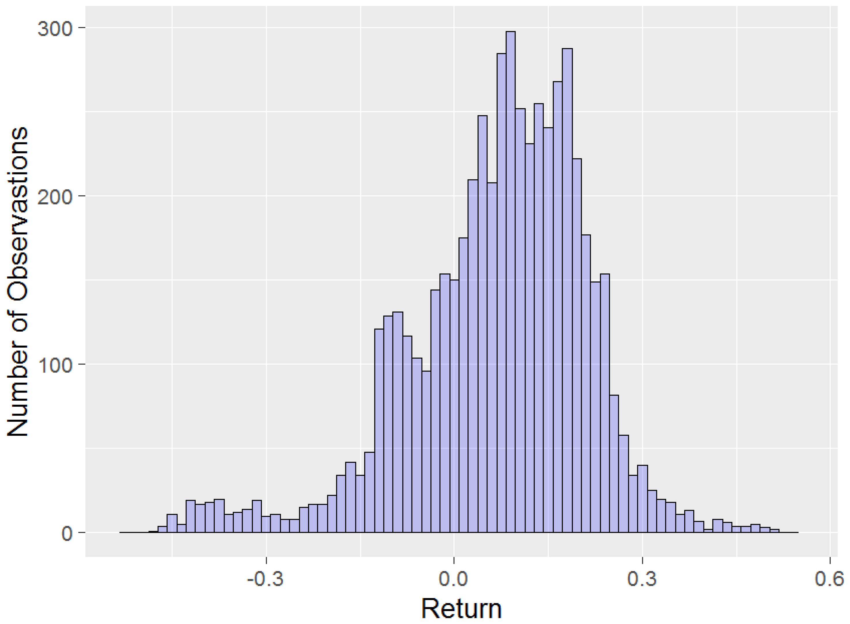
The advantage of using overlapping return data is that the range of possible annual returns depending on the annual calendar point when decisions are made is captured. However, a consequence of using overlapping data is that the individual observations in Figure 1 are not independent of each other. Whilst this will not bias the summary statistics estimates (with the exception that daily returns in the first and last years of the sample will not appear in the rolling annual return data with the same frequency as other years), it does mean that the distribution of returns will not be truly representative of a full 5566 independent observations. This is only likely to be noticeable in the tails of the distribution, with extremely rare events unlikely to be representative of independent observations. However, since we are not trying to fit econometric models to this overlapping data (see for example Lyon et al. 1999), and are more interested in expectations than in the tail of the distribution, this is not a particularly big issue. A histogram of the data is presented in Figure 1.
3.1. Alternative Calculations of
As a baseline, we assume that a value of from Equation (3), based on the mean from all 5566 observations of the equity return, is our target. Of course, using all 5566 observations to determine is computationally prohibitive for more complex problems, in general, but not for the simple model used in this paper. We will call this the Base (B) scenario and give all other scenarios below appropriate labels. This Base scenario can be approximated as an average:
where is the density function for a functional form of the equity return distribution, and is the value of the objective when the equity return is j. In the estimation of the integral is the equity return for the kth observation from the data. can be determined by calculating from Equation (2) and using the previously calculated values in the recursive process (using interpolation between values—see Section 2).
Our goal is to find the method of estimating that gives results closest to Base. All approaches use the following basic structure, with S representing the scenario being tested, representing the kth observed equity return from that scenario, and representing the weight attached to that observed equity return:
We now describe the scenarios to be tested. Similarly to Blake et al. (2013), a value of is used (i.e., 9 nodes are used). We complete the subsection with Table 1 and Table 2, which outline the equity return nodes, weights and summary statistics respectively for the calculations described below. Note that the Base results in Table 2 provide the summary statistics from the histogram in Figure 1.
3.1.1. Normal Distribution Quadrature (NQ)
The NQ scenario assumes from Equation (6) is normal with mean 6.92% and 14.46%, as estimated from the historical real equity return data (unrounded numbers are used in all modelling in the paper). A Gauss-Hermite process is used to determine and values, noting that, in this and other relevant scenarios, the component of the weights typically associated with Gauss-Hermite processes has been rolled into in order to provide a consistent comparison between scenarios.
3.1.2. Lognormal Distribution Quadrature (LQ)
The approach here is essentially the same as NQ, although the normal distribution is fitted to the continuously compounded , leading to 5.66% and 14.86% in the lognormal distribution. Again a Gauss-Hermite process is used to determine (converted back to effective rates) and values.
3.1.3. Data-Driven with Equal-Interval Nodes (DE)
Given that in Equation (7) is analogous to , it makes sense to treat as estimates of the relative frequency for which each occurs in the data. This can be easily done by splitting the equity return data between the minimum and maximum equity return into n clusters of equal-interval, with representing the proportion of the 5566 equity return observations in that cluster. The values are calculated as the mean return of the equity return observations in that cluster. The estimation is hence being treated as a Riemann integral (otherwise known as the infinite limit of a sum of rectangular rule approximations). We did consider allowing to be the mid-point of the cluster observations rather than the mean, but found the results in Section 3.2 to be inferior. One attractive feature of using the mean of cluster observations is that it ensures the weighted mean of the values is equal to the mean of the data.
3.1.4. Data-Driven with Unequal-Interval Nodes (DU)
We would like to investigate whether using nodes of unequal-interval, as done in , in combination with historical data, has a positive impact on results compared to above. In determining , we first identify from Equation (7) and then set the boundaries defining the clusters by which the proportion values are calculated to be halfway between consecutive values (and setting the minimum and maximum boundaries for the first and last nodes as and respectively). Like for DE above, we then set to be equal to the mean return of the equity return observations in each cluster.
3.2. Results
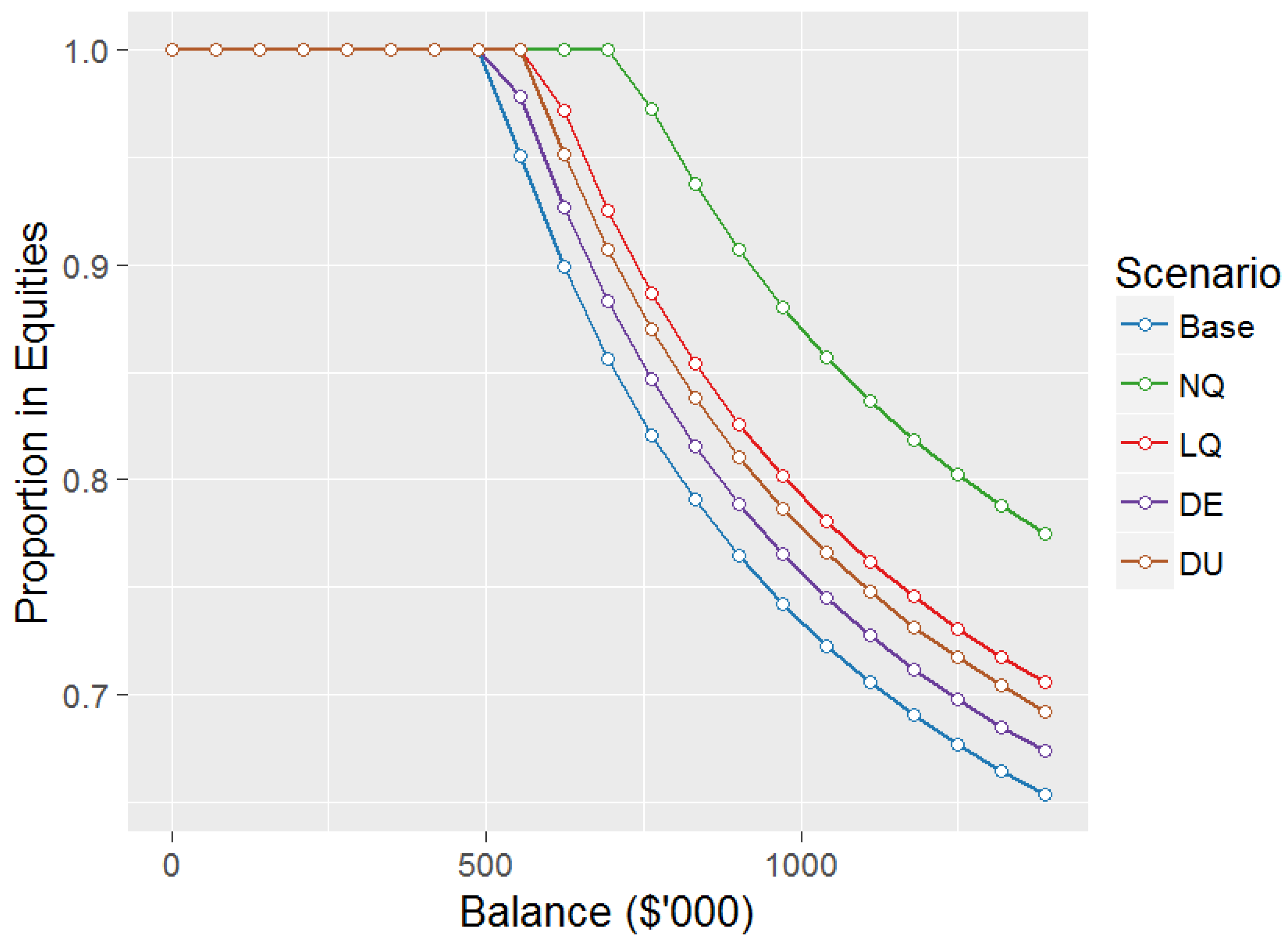
We start by looking at the optimal allocation to equities at age 55 for the Base and other scenarios, as shown in Figure 2.
The shape of the equity allocations at age 55 are consistent with Butt and Khemka (2015), with the 100% equity allocation constraint applying at smaller balances and then a decreasing equity allocation as balance increases. The decreasing equity allocation is due to future labour income being effectively a risk-free asset, and hence a higher balance requires a lower allocation to equities to maintain a consistent portfolio risk (see Bodie et al. 1992).
Asset allocations for other ages are not shown, although it can be noted that as age increases from age 55 the proportion of balance allocated to equities falls for a given balance until reaching the asymptotic values of 43.3%, 51.3%, 46.8%, 44.7%, and 45.9%, for scenarios , and respectively, which are maintained for all ages from age 65 onwards (with minor decreases with age due to the maximum age 110), as per Samuelson (1969). This trend is due to future labour income dropping to zero at age 65.
Interestingly the Base scenario has the lowest equity allocation of all scenarios, with data-driven scenarios and being closest to Base, and normal quadrature () having up to 15% higher allocation to equities for age 55. The lack of excess kurtosis in the normal distribution as compared to the data appears to be a significant factor in this difference.
We will now consider optimal consumption decisions. As per Samuelson (1969), consumption for an individual without labour income (i.e., from age 65 onwards) is a fixed proportion of balance, with the proportion for the Base scenario being 4.37%, 5.55%, 7.76%, and 11.80% for ages 65, 75, 85, and 95 respectively). For the Base scenario at age 55 and balance zero it is optimal to consume $28,311 of the $85,000 salary (the remainder being contributed to the balance), with optimal consumption increasing by an almost linear $0.0369 for every $1 of increase in balance (the number is slightly larger than this when the 100% (no borrowing) constraint for equity allocation applies).
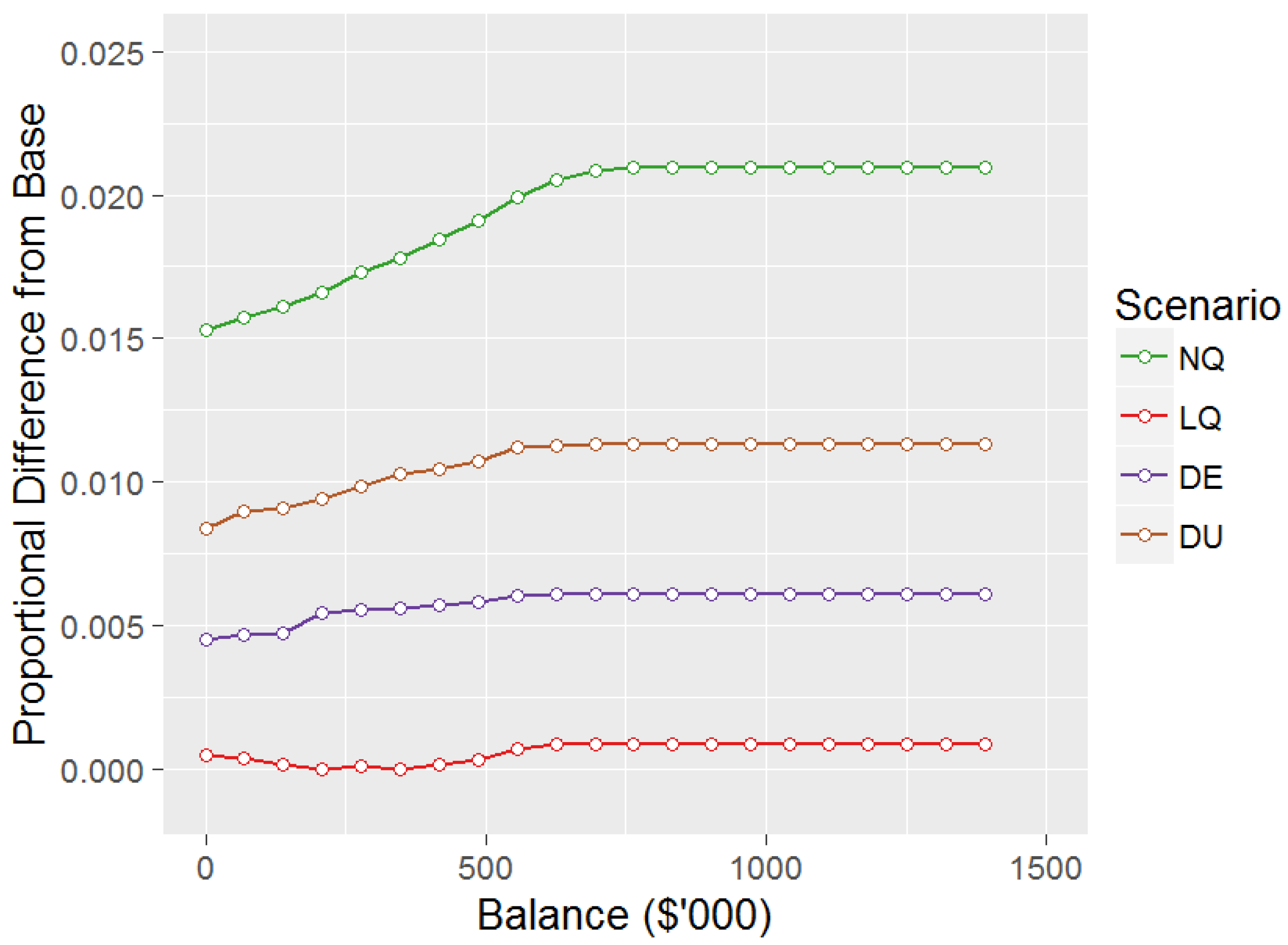
Figure 3 shows the proportional differences in consumption for the other scenarios compared to the Base scenario for age 55. Consistent with the equity allocation results in Figure 2 the consumption levels are higher as a proportion of balance for all scenarios compared to Base, with being the highest and consuming 2.10% higher than Base at age 55 when the 100% equity allocation constraint does not apply. However, the order of level of consumption is not the same as the order of level of equity allocation, with having almost identical consumption to Base, whilst having the second highest equity allocation in Figure 2. Differences between Base and other scenarios vary at other ages, with the difference tending to be increasing at younger ages, before decreasing from around age 45–50, although the order of the scenarios described above is maintained.
Whilst the above results are interesting in of themselves, due to the interaction between optimal equity allocation and consumption (e.g., as described in the previous paragraph), they do not give us sufficient information to determine which scenario gives us the closest results to Base. In order to determine this, we now perform a forward looking simulation exercise using 556,600 simulations, with utility in a given simulation calculated as per Equation (1), and using the optimal decisions for each scenario as described above. Linear interpolation is used to determine optimal equity allocations and consumption amounts between the balance nodes, with linear extrapolation of the final two nodes being used where the simulated balance exceeds the maximum balance node. Constraints on consumption and asset allocation as per the optimal decisions are applied. In generating the equity returns for the simulations, the 5566 equity return observations of the Base scenario are replicated 100 times, giving 556,600 observations, which are then random allocated without replacement to the 556,600 simulations, with this procedure being performed separately for each age. This ensures that the distribution of equity returns for the simulation exercise is identical to the Base equity return data at each age, although in any given simulation the distribution of equity returns across ages will depend on which observations are selected for each age for that simulation. The exercise is performed separately for starting ages from 25–64, with the starting balance assumed to be zero for each age. The expected utility for a given scenario is calculated as the mean utility across 556,600 simulations.
Since the simulations are based on equity return data consistent with the Base scenario, the Base decisions give the best utility outcomes. Figure 4 presents a comparison of the proportionate difference in utility outcomes for the other scenario decisions as compared to Base, for each age from 25–64 all starting from a zero balance. Scenarios which give values closest to Base (i.e., closest to zero in Figure 4) represent the best scenarios to use.
It is clear from Figure 4 that the data-driven approaches perform better than quadrature approaches in maximising utility as compared with the Base scenario, with equal-interval nodes having a utility only 0.09% worse than Base for age 25 and initial balance zero, compared to 0.27% for , 0.48% for and 1.92% for . This is quite an exciting result, with the reduction from 5566 equity return observations to 9 equity return nodes giving almost no loss in utility. Despite the unequal-interval approach having only 7 effective nodes (see Section 3.1) it still performs better than either of the quadrature approaches. The poor performance of is unsurprising given it gave the greatest difference in optimal decisions in Figure 2 and Figure 3. Trends with age in utility outcomes compared to Base can be explained by two factors. Firstly, the impact of the 100% equity allocation means that for much of the pre-retirement for younger starting ages equity allocations under all scenarios are 100%, giving a smaller utility difference for these starting ages. However, at very young starting ages the balance increases to a large enough amount that the large differences seen in equity allocations for larger balances in Figure 2 start applying, explaining the very slight downward trend at younger ages for . Secondly, the reduction in the moderating influence of future salaries as age increases tends to increase the difference between Base and the other scenarios.
Finally, in addition to the results described above, each of the above scenarios was tested for and nodes. Whilst detailed results are not presented here for reasons of brevity, the utility difference compared to Base for age 25 initial balance zero for nodes is 1.92%, 0.48%, 0.62%, and 0.70%, and for nodes is 1.92%, 0.48%, 0.02%, and 0.12%, for scenarios , and respectively. This shows that 5 nodes is sufficient for no further change in quadrature results with additional nodes (and in fact performs better than data-driven approaches for only 5 nodes), whilst data-driven approaches move even closer to Base with more nodes.
4. The Multiple Stochastic Asset Setting
The individual in the model is assumed to have a choice between four stochastic assets, namely domestic equities, international equities, domestic bonds and international bonds. Hence from Equation (2) is now calculated as follows:
where , , and are the stochastic equity returns for domestic equities, international equities, domestic fixed interest and international fixed interest, respectively, and , , and , are the equivalent asset allocation proportions at age x. The optimisation problem in Equation (3) is now controlled upon , , and , and is constrained upon (i.e., no short selling or borrowing constraint), , and, for , .
In determining historical data structures on which to base the four asset class return structures, we initially used international equity (MSCI Developed World Equity Index), fixed interest (Bloomberg Australia Bond Composite 0+ Year Index) and cash (UBS AU Bank Bill All Maturities Index) returns, in addition to the domestic equity returns from Section 3. However, we discovered that using these asset classes tended to lead to optimal decision making dominated by domestic equities and fixed interest allocations, with essentially zero allocation to international equity (which had lower mean returns and higher standard deviation than domestic equities) and cash (which had much lower mean returns which failed to compensate for the lower standard deviation compared to fixed interest).
Given the purpose of this paper, we felt it would be beneficial to select asset classes that gave non-trivial optimal allocations to each of the four asset classes. This proved to be more challenging than we expected, with a number of candidate asset classes being investigated before settling on U.S. domestic equities (S&P 500 Equity Index), Australian Equities as international equities (S&P/ASX200 Accumulation Index unhedged in $US), U.S. domestic fixed interest (US Government Bond Indices > 1 Year total returns) and Italian Government bonds as international fixed interest (Italian Government Bond Indices > 1 Year total return unhedged in $US). Again real (with respect to the US Personal Income Index) daily, rolling annual returns from 1 January 1993 to 31 December 2015 were used to give us 5522 observations across four assets (the number of observations is reduced from the 5566 in Section 3 due to public holidays needing to be taken into account for three countries rather than one). Some summary statistics of the data are presented in Table 3.
4.1. Alternative Calculations of
Like in Section 3.1, we set from Equation (3) in the Base (B) scenario to be the mean from all 5522 observations of the four assets. This Base scenario is expressed as:
In Equation (9), is the multivariate density function for a functional form of the domestic equity (), international equity (), domestic fixed interest () and international fixed interest () return distribution, and is the value of the objective when the returns are , , and . In the estimation of the integral is now the vector of returns for the kth observation from the data. is calculated in the equivalent way as in Section 3. Note that this approach maintains cross-correlation between assets but not autocorrelation across time in the model (a topic for future research; see Section 5). Again our goal is to find the method of estimating that gives results closest to Base.
4.1.1. Weighted Nodes—Quadrature
We will start with quadrature approaches like we did in Section 3, with S representing the scenario being tested and other notation consistent with Section 3 and above:
However, were we to allow for the intersection of 9 nodes across four variables, this would give us 6561 summation elements, which is more than the 5522 historical data points, and so is not of interest as it would be more computationally intensive than Base.
We wish to use more nodes for assets with higher volatility and so we choose , , and as the number of nodes used. This gives a multiplied total of 2025 nodes. For reasons of brevity, unlike the single stochastic asset formulation in Section 3.1 no summary statistics will be provided for the approaches described in this section, although they can obtained from the authors on request.
Weighted Nodes—Normal Distribution Quadrature (WN-NQ)
We start by considering a normal distribution quadrature version of this approach . In order to allow for correlation between the asset classes, we perform a Cholesky decomposition of the variance/covariance matrix of the 5522 historical data points, as per Cai and Judd (2010), giving us an independent normal distribution for the residuals of each asset class. The calculation of is a product Gauss-Hermite quadrature to determine the and values from Equation (10), as per Cai and Judd (2010).
Weighted Nodes—Lognormal Distribution Quadrature (WN-LQ)
The lognormal distribution quadrature version of this approach is essentially the same as , although in this case the Cholesky decomposition is performed on the continuously compounded for each asset class. Again a product Gauss-Hermite process is used to determine the (converted back to effective rates) and values from Equation (10).
4.1.2. Weighted Nodes—Data-Driven
An alternative to Equation (10) is needed for data-driven approaches. Instead of the correlations between asset classes being represented by a Cholesky decomposition, we create joint clusters of the data and use the varying proportions of data in the joint clusters to represent the correlation. This is represented as follows:
where represents the proportion of the 5522 observations in that joint cluster across the four asset classes, whilst represents the vector of mean returns of the observations of the four asset classes in that joint cluster. We now need to decide how to define the joint clusters upon which and are to be based.
Weighted Nodes—Data-Driven and Equal-Interval Grid (WN-DE-G)
For we will start with equal-interval clusters in a way consistent to what we did in Section 3.1, using a naïve grid-based approach.Independently for each asset class we now split the return data between the minimum return and maximum returns into equal-interval clusters, giving joint clusters.
Structuring the grid in this way means that 1773 of the 2025 joint clusters contain no data (i.e., for many joint clusters), with the result that the effective number of nodes in WN-DE-G is only 252.
Weighted Nodes—Data-Driven and Equal-Interval Hierarchy (WN-DE-H)
An alternative approach to the naïve grid-based approach described above is to cluster using a divisive hierarchy (see Fraley and Raftery 1998). We start with all 5522 observations in a single cluster, and then separate the data into clusters based on the equal-interval approach described above applied to the observed returns only (i.e., the cluster is not dependent on the other asset class returns in any way). Then we split each of the -based clusters into clusters based on returns only, performing the equal-interval approach separately for each of the -based clusters (i.e., the range of data in the equal-interval clusters differs depending on the data in each of the -based clusters). Similarly, we then split each of the --based clusters into clusters, and then split each of the ---based clusters into clusters, giving joint clusters.
Similarly to , in 1077 of the 2025 joint clusters contain no data, with the result that the effective number of nodes in is only 948. The much larger number of effective nodes is due to the hierarchical clustering setting different cluster ranges tailored to data location. Note that the hierarchy order could be different to that described above, although based on the results in Section 4.2 we don’t believe this would have a significant impact.
Weighted Nodes—Data-Driven and Unequal-Interval Grid (WN-DU)
In a similar way to in Section 3.1 we first identify independently for each univariate asset class, setting the boundaries defining the clusters to be halfway between consecutive values (and setting the minimum and maximum boundaries for the first and last nodes in each asset class as and respectively), again giving joint clusters.
Similarly to and , in 1851 of the 2025 joint clusters contain no data, with the result that the effective number of nodes in is only 174. This has a pleasant side effect of reducing computational time for the optimisation results in Section 4.2. We have not reported this previously as it is not a primary purpose of the paper, since all scenarios apart from Base have been initially set up to be equally computationally intensive. However, we can report that using R and the DEoptim package, the time for optimisation is s for respectively.
Note that an unequal-interval hierarchical approach is not possible, as it would require normal distributions to be fit separately to data throughout the hierarchy, which is not sensible (or sometimes even possible) for the small number of observations in parts of the hierarchy.
4.1.3. Quasi-Monte Carlo
Quasi-Monte Carlo () approaches have been found to be useful for estimating multidimensional integrals that otherwise would face the curse of dimensionality suffered by the quadrature approaches described above (see Dick et al. 2013). (A approach was not considered in Section 3.1 as Equation (6) is not a multidimensional integral.)
approaches are analogous to the equally weighted estimation in Equation (9), calculated as follows:
In Equation (12) r is the number of observations chosen, whilst is the asset class return vector for the Sth QMC observation chosen. In a approach, rather than a random simulation (or bootstrap for data-driven) approach, the choice of for which is calculated is via a deterministic process designed to improve upon a random approach. In order to be consistent with above we assume .
Since methods are applied to integrals across a multi-dimensional unit cube, the values for which are chosen will be based on cumulative densities. These values are determined from a four-dimensional Halton sequence (see Halton 1964), with a S value having the structure . Halton sequences assume independence between the multi-dimensional variables, hence we need to structure the data in such a way as to allow for this.
Quasi-Monte Carlo—Normal Distribution (QMC-N)
A Cholesky decomposition identical to that described for above is used, with the values from Equation (12) being determined from the normally converted S values, then correlated through the Cholesky decomposition.
Quasi-Monte Carlo—Lognormal Distribution (QMC-L)
The approach is identical to that described for through Equation (12) above, although in this case the Cholesky decomposition is performed on the continuously compounded for each asset class, with the values being determined from the normally converted S values, then correlated through the Cholesky decomposition and converted back to effective rates.
Quasi-Monte Carlo—Data-Driven (QMC-D)
For the observed independent residuals from the Cholesky decomposition are ordered, with the values in Equation (12) being determined from the observed residual percentiles based on the S values, then correlated through the Cholesky decomposition.
Note that only one data-driven approach is tested, as the concept of the spacing of nodes is irrelevant in .
4.2. Results
For reasons of brevity, in the multiple stochastic asset setting, we have not provided the results corresponding to Figure 2 and Figure 3, although they can be obtained from the authors on request. (Note the “Retiring” package described at the conclusion of the paper provides the equivalent figures in Figures A1–A3). It is to be noted that these results were not materially different to those seen in Section 3.2.
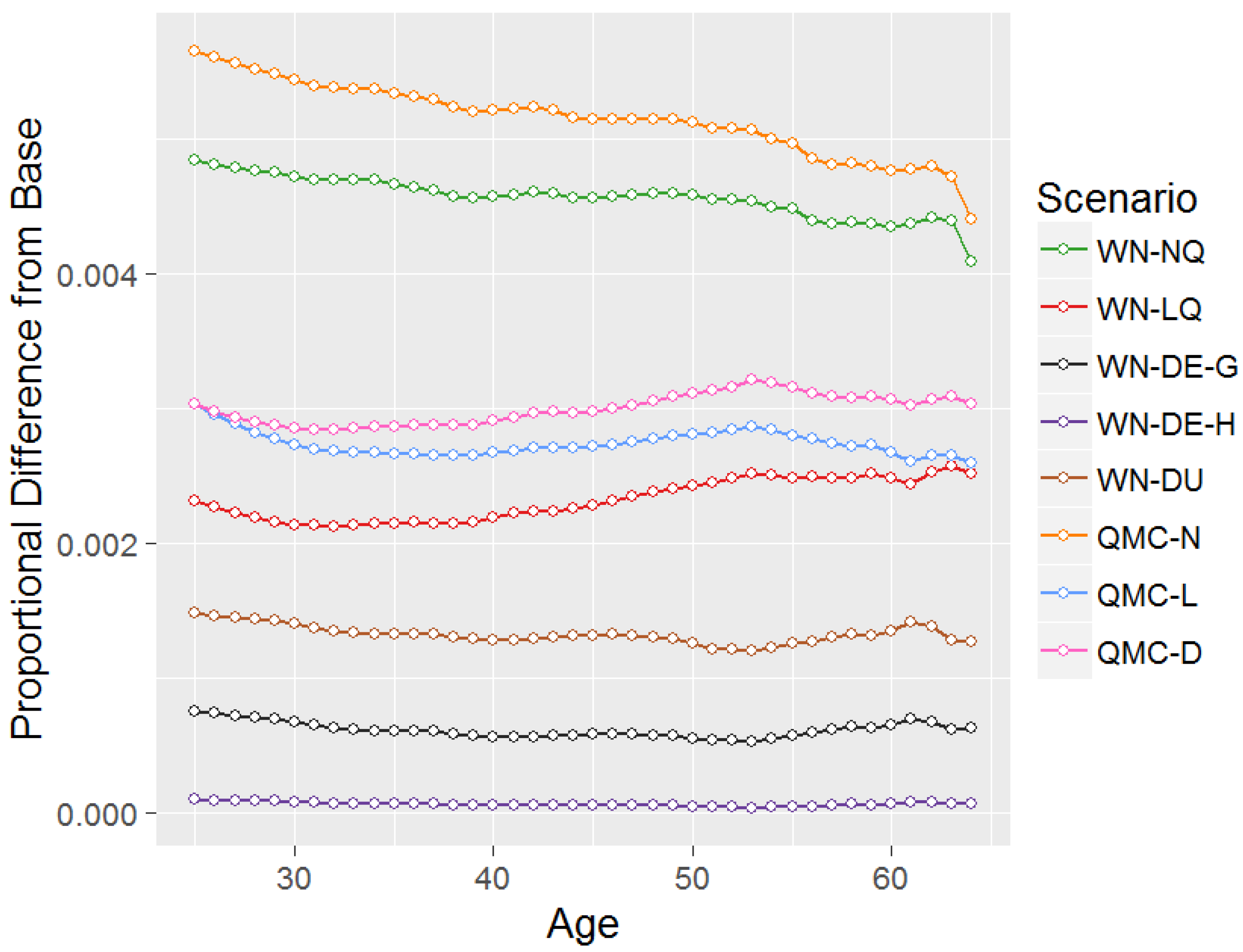
In order to determine which scenario gives the closest results to Base, a simultion exercise is performed, consistent with that described in Section 3.2, with 552,200 simulations performed based on the 5522 data observations. Figure 5 presents a comparison of the proportionate difference in utility outcomes for the other scenarios as compared to Base, for each age from 25–64 all starting from a zero balance.
With the exception of the poor results for NQ in Figure 4, the scale of difference between the utility results for Base and other scenarios is broadly similar for multiple stochastic assets in Figure 5 as it is for single stochastic assets in Figure 4. It is again clear from Figure 5 that the data-driven approaches perform the best compared to the Base scenario, with the equal-interval hierarchical-based approach, , having utility only 0.01% worse than Base for age 25 and initial balance zero, and grid-based approaches, and , giving differences of 0.08% and 0.15% respectively. This is a fantastic result given that the data-driven approaches are also more efficient than the other approaches, using 948, 252 and 174 nodes for , and respectively, compared to 2025 nodes for the other scenarios. The and results show that equal-interval grids perform better than unequal-interval grids, which is consistent with the results of single stochastic assets in Figure 4.
Conversely, Quasi-Monte Carlo approaches perform particularly poorly, with drops in utility compared to Base for age 25 and initial balance zero of 0.57%, 0.30% and 0.30% for , and respectively. Consistent with the results of single stochastic assets in Figure 4, the quadrature approach using a log-normal distribution, , performs much better at 0.23% than using a normal distribution, , at 0.48%.
Trends with age in utility outcomes compared to Base are not particularly strong. Bumps seen in the trends at later starting ages, particularly in and , are a result of idiosyncrasies in the optimisation procedure leading to very small deviations away from the correct optimal asset allocation and consumption results, but these do not have any material effect on the interpretation of the results.
Note that, in addition to the results described above, each of the above scenarios was tested for a smaller collection of , , and giving a multiplied total of 225 nodes. Given the possibility of zero data in joint clusters, as described in Section 4.1, the effective number of nodes for , and are 180, 76 and 78 respectively. Whilst detailed results are not presented here for reasons of brevity, the utility difference compared to Base for age 25 initial balance zero is 0.48%, 0.23%, 0.14%, 0.71%, 0.44%, 1.33%, 1.51%, and 1.23% for scenarios , and respectively. In a similar way to single stochastic assets, this shows that 225 nodes is sufficient for no further change in quadrature results with additional nodes, whilst data-driven approaches move closer to Base with more nodes.
5. Conclusions and Future Research
This paper considers an alternative way of structuring stochastic variables in a dynamic programming framework where the model structure dictates that numerical methods of solution are necessary. Rather than estimating integrals within a Bellman equation using quadrature nodes from a distribution fit to underlying data, we use nodes directly from the underlying data. An example of the application of this approach is presented using individual lifetime financial modelling.
The results show that determining nodes directly from the data provides results far closer to a base scenario which uses all data points, than determining nodes from fitted distributions or using a Quasi-Monte Carlo approach. These results hold for both a single stochastic variable and multiple stochastic variables, with an added benefit for multiple stochastic variables of using far less nodes than a quadrature approach.
There is a wealth of potential future research that could follow from this work. Our method is broadly applicable to any dynamic programming problem involving stochastic and time-based assumptions. That said, what we have demonstrated in this paper is very basic, and could be expanded upon in a variety of ways.
For example, the clustering methods employed are very simple, and could potentially be improved upon by options such as k-means clustering or other approaches (see Fraley and Raftery 1998). Comparisons between the data-driven approach and alternative quadrature approaches, such as the use of sparse grids (see Heiss and Winschel 2008) rather than product rules, could also be performed for multiple stochastic assets. Future work could also look at the impact of using non-parametric estimates of the entire density function , such as those described in the seminal work of Parzen (1962), and combining them with other Newton-Cotes estimations.
Furthermore, incorporation of autocorrelation in the data could lead to interesting insights for various problems. Some prior papers have considered this issue. For example, Campbell et al. (2003) use a vector autoregressive process to analytically solve a simple consumption and asset allocation problem. Kopcke et al. (2013) extends this model to incorporate social security benefits and uncertain labour market earnings, requiring numeric methods of solution. The approach in this paper could certainly be applied to vector autoregressive processes, or structured cascade relationships like Wilkie (1995), although in these cases the “data” would be the residuals of these processes rather than the underlying data, in a similar way to bootstrapping residuals (see page 113 of Efron and Tibshirani 1994).
Given the wide application of dynamic programming in many research and commercial areas, we consider that the approach demonstrated in this paper will be of considerable interest to a wide variety of researchers and practitioners, and look forward to these and other future developments in this area.
Supplementary Materials
The following are available online at www.mdpi.com/2227-9091/5/4/57/s1, R-package ‘Retiring’ containing the code to perform the diagnostic methods and generate the outputs described in the paper. The package also contains all datasets used as examples in the paper. Please read the “User Guide” for instructions on the use of the package. A file entitled “Example commands for ‘Retiring’ package” is also provided for ease of use.
Acknowledgments
The authors gratefully acknowledge the 2016 Vice-Chancellor’s Research Seed Grant from Bond University and the 2015–16 Research School Grant from Australian National University. The authors would also like to acknowledge the help of their research assistant, Mr. James Todd for the help offered in writing the R-code that was invaluable in generating the outputs for this paper.
Author Contributions
A.B. and G.K. concieved and designed the paper. A.B. did the main bulk of writing the paper. G.K. did the main bulk of generating the results.
Conflicts of Interest
The authors declare no conflict of interest.
Abbreviations
The following abbreviations are used in this manuscript:
| ASX | Australian Stock Exchange |
| AU | Australia |
| AWE | AverageWeekly Earnings |
| CRRA | Constant Relative Risk Aversion |
| DE | Data-driven with Equal-interval nodes |
| DU | Data-driven with Unequal-interval nodes |
| LQ | Lognormal distribution Quadrature |
| MDPI | Multidisciplinary Digital Publishing Institute |
| MSCI | Morgan Stanley Capital International |
| NQ | Normal distribution Quadrature |
| QMC | Quasi-Monte Carlo |
| QMC-D | Quasi-Monte Carlo - Data-driven |
| QMC-L | Quasi-Monte Carlo - Lognormal distribution |
| QMC-N | Quasi-Monte Carlo - Normal distribution |
| S&P | Standard & Poor’s |
| UBS | Union Bank of Switzerland |
| US | the United States of America |
| WN-DE-G | Weighted Nodes-Data-driven and Equal-interval Grid |
| WN-DE-H | Weighted Nodes-Data-driven and Equal-interval Hierarchy |
| WN-DU | Weighted Nodes-Data-driven and Unequal-interval grid |
| WN-LQ | Weighted Nodes-Lognormal distribution Quadrature |
| WN-NQ | Weighted Nodes-Normal distribution Quadrature |
References
- Australian Government Actuary. 2014. Australian Life Tables 2010-12; Canberra: Commonwealth of Australia.
- Bellman, Richard. 1957. Dynamic Programming, 1st ed. Princeton: Princeton University Press. [Google Scholar]
- Blake, David, Douglas Wright, and Yumeng Zhang. 2013. Target-driven investing: Optimal investment strategies in defined contribution pension plans under loss aversion. Journal of Economic Dynamics and Control 37: 195–209. [Google Scholar] [CrossRef]
- Bodie, Zvi, Robert C. Merton, and William F. Samuelson. 1992. Labor supply flexibility and portfolio choice in a life cycle model. Journal of Economic Dynamics and Control 16: 427–49. [Google Scholar] [CrossRef]
- Boyle, Phelim, Junichi Imai, and Ken Seng Tan. 2002. Asset Allocation Using Quasi Monte Carlo Methods. Working paper, University of Waterloo, Waterloo, ON, Canada. [Google Scholar]
- Butt, Adam, and Gaurav Khemka. 2015. The effect of objective formulation on retirement decision making. Insurance: Mathematics and Economics 64: 385–95. [Google Scholar] [CrossRef]
- Cai, Yongyang, and Kenneth L. Judd. 2010. Stable and efficient computational methods for dynamic programming. Journal of the European Economic Association 8: 626–34. [Google Scholar] [CrossRef]
- Campbell, John Y., Yeung Lewis Chan, and Luis M. Viceira. 2003. A multivariate model of strategic asset allocation. Journal of Financial Economics 67: 41–80. [Google Scholar] [CrossRef] [Green Version]
- Carroll, Christopher D. 2006. The method of endogenous gridpoints for solving dynamic stochastic optimization problems. Economics Letters 91: 312–20. [Google Scholar] [CrossRef]
- Dick, Josef, Frances Y. Kuo, and Ian H. Sloan. 2013. High-dimensional integration: The quasi-monte carlo way. Acta Numerica 22: 133–288. [Google Scholar] [CrossRef]
- Efron, Bradley, and Robert J. Tibshirani. 1994. An Introduction to the Bootstrap. Boca Raton: CRC Press. [Google Scholar]
- Fama, Eugene F. 1965. The behavior of stock-market prices. The Journal of Business 38: 34–105. [Google Scholar] [CrossRef]
- Fraley, Chris, and Adrian E. Raftery. 1998. How Many Clusters? Which Clustering Method? Answers via Model-Based Cluster Analysis. The Computer Journal 41: 578–88. [Google Scholar] [CrossRef]
- Gerrard, Russell, Steven Haberman, and Elena Vigna. 2006. The management of decumulation risks in a defined contribution pension plan. North American Actuarial Journal 10: 84–110. [Google Scholar] [CrossRef]
- Haberman, Steven, and Elena Vigna. 2002. Optimal investment strategies and risk measures in defined contribution pension schemes. Insurance: Mathematics and Economics 31: 35–69. [Google Scholar] [CrossRef]
- Halton, John H. 1964. Algorithm 247: Radical-inverse quasi-random point sequence. Communications of the ACM 7: 701–2. [Google Scholar] [CrossRef]
- Hanewald, Katja, John Piggott, and Michael Sherris. 2013. Individual post-retirement longevity risk management under systematic mortality risk. Insurance: Mathematics and Economics 52: 87–97. [Google Scholar] [CrossRef]
- Heiss, Florian, and Viktor Winschel. 2008. Likelihood approximation by numerical integration on sparse grids. Journal of Econometrics 144: 62–80. [Google Scholar] [CrossRef] [Green Version]
- Horneff, Vanya, Raimond Maurer, Olivia S. Mitchell, and Ralph Rogalla. 2015. Optimal life cycle portfolio choice with variable annuities offering liquidity and investment downside protection. Insurance: Mathematics and Economics 63: 91–107. [Google Scholar] [CrossRef]
- Hulley, Hardy, Rebecca Mckibbin, Andreas Pedersen, and Susan Thorp. 2013. Means-tested public pensions, portfolio choice and decumulation in retirement. Economic Record 89: 31–51. [Google Scholar] [CrossRef]
- Kopcke, Richard W., Anthony Webb, and Joshua Hurwitz. 2013. Rethinking Optimal Wealth Accumulation and Decumulation Strategies in the Wake of the Financial Crisis. Working paper, Center for Retirement Research at Boston College, Chestnut Hill, MA, USA. [Google Scholar]
- Korn, Ralf, Tak Kuen Siu, and Aihua Zhang. 2011. Asset allocation for a dc pension fund under regime switching environment. European Actuarial Journal 1: 361–77. [Google Scholar] [CrossRef]
- Lyon, John D., Brad M. Barber, and Chih-Ling Tsai. 1999. Improved methods for tests of long-run abnormal stock returns. The Journal of Finance 54: 165–201. [Google Scholar] [CrossRef]
- Merton, Robert C. 1969. Lifetime portfolio selection under uncertainty: The continuous-time case. The Review of Economics and Statistics 51: 247–57. [Google Scholar] [CrossRef]
- Michaelides, Alexander, and Yuxin Zhang. 2015. Stock market mean reversion and portfolio choice over the life cycle. Journal of Financial and Quantitative Analysis 52: 1183–209. [Google Scholar] [CrossRef]
- Parzen, Emanuel. 1962. On estimation of a probability density function and mode. The Annals of Mathematical Statistics 33: 1065–76. [Google Scholar] [CrossRef]
- Pirvu, Traian A., and Huayue Zhang. 2012. Optimal investment, consumption and life insurance under mean-reverting returns: The complete market solution. Insurance: Mathematics and Economics 51: 303–9. [Google Scholar] [CrossRef]
- Poterba, James M., and Lawrence H. Summers. 1988. Mean reversion in stock prices. Journal of Financial Economics 22: 27–59. [Google Scholar] [CrossRef]
- Samuelson, Paul A. 1969. Lifetime portfolio selection by dynamic stochastic programming. The Review of Economics and Statistics 51: 239–46. [Google Scholar] [CrossRef]
- Shapiro, Arnold F. 2010. Post-Retirement Financial Strategies from the Perspective of an Individual Who Is Approaching Retirement Age. Society of Actuaries 71: 74. [Google Scholar]
- Wilkie, A. David. 1995. More on a stochastic asset model for actuarial use. British Actuarial Journal 1: 777–964. [Google Scholar] [CrossRef]
- Yaari, Menahem E. 1987. The dual theory of choice under risk. Econometrica 55: 95–115. [Google Scholar] [CrossRef]
- Zou, Bin, and Abel Cadenillas. 2014. Explicit solutions of optimal consumption, investment and insurance problems with regime switching. Insurance: Mathematics and Economics 58: 159–67. [Google Scholar] [CrossRef]
Figure 1.
Histogram of real domestic equity returns from the historical data.

Figure 2.
Equity allocation for age 55.

Figure 3.
Consumption comparisons between Base and other scenarios for age 55.

Figure 4.
Utility comparisons between Base and other scenarios for an initial balance of zero.
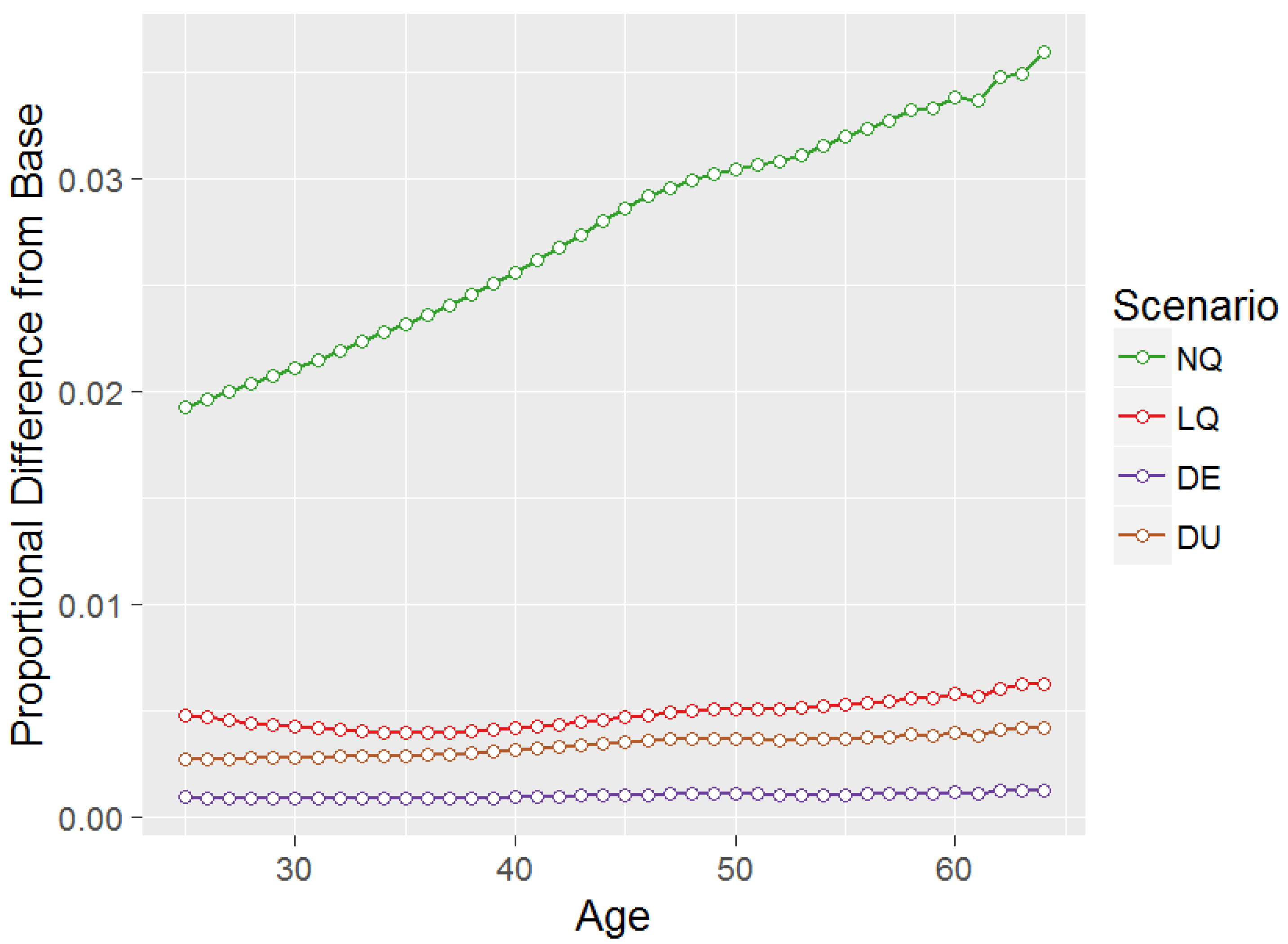
Figure 5.
Utility comparisons between Base and other scenarios for an initial balance of zero.


Table 1.
Equity return nodes and weights for calculations.
| Number | NQ | LQ | DE | DU | ||||
|---|---|---|---|---|---|---|---|---|
| 1 | −58.34% | 0.00002 | −45.89% | 0.00002 | −41.35% | 0.01563 | N/A* | 0.00000 |
| 2 | −39.43% | 0.00279 | −34.29% | 0.00279 | −32.25% | 0.01671 | −38.37% | 0.02641 |
| 3 | −23.11% | 0.04992 | −22.28% | 0.04992 | −19.33% | 0.02911 | −21.11% | 0.03414 |
| 4 | −7.88% | 0.24410 | −9.11% | 0.24410 | −9.27% | 0.13223 | −7.00% | 0.19817 |
| 5 | 6.92% | 0.40635 | 5.82% | 0.40635 | 1.84% | 0.23733 | 7.46% | 0.41197 |
| 6 | 21.71% | 0.24410 | 23.20% | 0.24410 | 12.16% | 0.34765 | 19.74% | 0.30004 |
| 7 | 36.95% | 0.04992 | 44.09% | 0.04992 | 21.63% | 0.18829 | 34.29% | 0.02641 |
| 8 | 53.26% | 0.00279 | 70.40% | 0.00279 | 32.55% | 0.02695 | 47.84% | 0.00287 |
| 9 | 72.17% | 0.00002 | 106.95% | 0.00002 | 45.13% | 0.00611 | N/A * | 0.00000 |
* No data was observed in clusters 1 and 9 for DU, and so the effective number of nodes in DU is only 7.
Table 2.
Summary statistics of real equity returns from the calculations.
| Statistic | Base | NQ | LQ | DE | DU |
|---|---|---|---|---|---|
| Arithmetic mean (p.a.) | 6.92% | 6.92% | 6.99% | 6.92% | 6.92% |
| Standard deviation (p.a.) | 14.46% | 14.46% | 15.99% | 14.14% | 13.91% |
| Skewness | −0.8023 | 0.0000 | 0.4517 | −0.8619 | −0.8801 |
| Kurtosis (Excess) | 1.3743 | 0.0000 | 0.3649 | 1.5314 | 1.5602 |
Note: p.a. stands for per annum.
Table 3.
Summary statistics of real returns from the historical data.
| Statistic | Arithmetic Mean (p.a.) | Standard Deviation (p.a.) | Skewness | Kurtosis (Excess) |
|---|---|---|---|---|
| Domestic Equities (ed) | 5.76% | 16.52% | −0.4437 | 0.3886 |
| International Equities (ei) | 7.66% | 23.00% | 0.7391 | 3.5079 |
| Domestic Fixed Interest (fd) | 0.94% | 5.02% | 0.3106 | −0.3217 |
| International Fixed Interest (fi) | 2.99% | 11.90% | 0.0464 | −0.2338 |
Note: p.a. stands for per annum.
© 2017 by the authors. Licensee MDPI, Basel, Switzerland. This article is an open access article distributed under the terms and conditions of the Creative Commons Attribution (CC BY) license (http://creativecommons.org/licenses/by/4.0/).
Share and Cite
MDPI and ACS Style
Khemka, G.; Butt, A. Non-Parametric Integral Estimation Using Data Clustering in Stochastic dynamic Programming: An Introduction Using Lifetime Financial Modelling. Risks 2017, 5, 57. https://doi.org/10.3390/risks5040057
AMA Style
Khemka G, Butt A. Non-Parametric Integral Estimation Using Data Clustering in Stochastic dynamic Programming: An Introduction Using Lifetime Financial Modelling. Risks. 2017; 5(4):57. https://doi.org/10.3390/risks5040057
Chicago/Turabian StyleKhemka, Gaurav, and Adam Butt. 2017. "Non-Parametric Integral Estimation Using Data Clustering in Stochastic dynamic Programming: An Introduction Using Lifetime Financial Modelling" Risks 5, no. 4: 57. https://doi.org/10.3390/risks5040057
Note that from the first issue of 2016, this journal uses article numbers instead of page numbers. See further details here.