A Novel Three-Stage Filter-Wrapper Framework for miRNA Subset Selection in Cancer Classification


1
Department of Computer Engineering, Faculty of Engineering, Lorestan University, Khoramabad 1489684511, Iran
2
Department of Computer Engineering, Faculty of Engineering, Yazd University, Yazd 891581-8411, Iran
3
Department of Electrical Engineering, Shahid Bahonar University of Kerman, Kerman 76169-14111, Iran
*
Author to whom correspondence should be addressed.
Informatics 2018, 5(1), 13; https://doi.org/10.3390/informatics5010013
Submission received: 2 November 2017
/
Revised: 20 February 2018
/
Accepted: 27 February 2018
/
Published: 1 March 2018
(This article belongs to the Special Issue Biomedical Informatics)
Abstract
:Micro-Ribonucleic Acids (miRNAs) are small non-coding Ribonucleic Acid (RNA) molecules that play an important role in the cancer growth. There are a lot of miRNAs in the human body and not all of them are responsible for cancer growth. Therefore, there is a need to propose the novel miRNA subset selection algorithms to remove irrelevant and redundant miRNAs and find miRNAs responsible for cancer development. This paper tries to propose a novel three-stage miRNAs subset selection framework for increasing the cancer classification accuracy. In the first stage, multiple filter algorithms are used for ranking the miRNAs according to their relevance with the class label, and then generating a miRNA pool obtained based on the top-ranked miRNAs of each filter algorithm. In the second stage, we first rank the miRNAs of the miRNA pool by multiple filter algorithms and then this ranking is used to weight the probability of selecting each miRNA. In the third stage, Competitive Swarm Optimization (CSO) tries to find an optimal subset from the weighed miRNAs of the miRNA pool, which give us the most information about the cancer patients. It should be noted that the balance between exploration and exploitation in the proposed algorithm is accomplished by a zero-order Fuzzy Inference System (FIS). Experiments on several miRNA cancer datasets indicate that the proposed three-stage framework has a great performance in terms of both the low error rate of the cancer classification and minimizing the number of miRNAs.
1. Introduction
Micro-Ribonucleic Acids (miRNAs) are small Ribonucleic Acids (RNA) molecules that play an important role in the cancer growth. There are more than one thousand miRNAs in the human body and only some of them are responsible for cancer growth. Therefore, there is a need to propose the novel methods to find a subset of responsible miRNAs, which helps us to obtain better classification when classifying a new patient. In the other words, it is necessary to remove irrelevant and redundant miRNAs from data and find an optimal subset of relevant miRNAs that gives us the most information about the cancer patients. There are many reasons why we should use the miRNA subset selection as a pre-processing phase for cancer classification:
- In most classification algorithms, the complexity of the algorithm depends on the dimensions of data. So, in order to reduce the memory and computational time, we are interested in removing the irrelevant and redundant miRNAs from the dataset.
- When it has been determined that a miRNA does not have a positive effect on the cancer diagnosis, the time and biochemical cost required to extract this miRNA can be saved. It should be noted that this can significantly accelerate the process of the cancer diagnosis.
- When it is possible to represent the data without losing the information in a small number of miRNAs, they can be plotted visually and this can help extracting the useful knowledge about cancer.
- When data are represented by fewer miRNAs, it is easier to analyze the processes that generate the data and this helps to extract useful knowledge about cancer.
One of the best ways to remove irrelevant and redundant miRNAs is to use the feature subset selection algorithms [1]. So far, the various algorithms have been proposed for feature subset selection. The first algorithm that comes to mind is the exhaustive search algorithm which tests all feature subsets one by one and then chooses the best feature subset. Although this algorithm has a simple logic, but directly evaluating all subsets of features generates an algorithm with exponential time complexity [2,3], because there are different feature subsets when we have a feature set with size d. Since it is not rational to use exhaustive search for high-dimensional feature subset selection, there are very few algorithms that use exhaustive search in feature space [1]. It is noteworthy that exhaustive search algorithms can only solve small and medium size datasets and cannot be used for miRNAs datasets because exhaustive search in high-dimensional space is practically impossible. In such a case, approximate methods are suggested to remove redundant and irrelevant miRNAs in a reasonable time [2]. The approximate feature subset selection algorithms can be classified into three categories: filter methods, wrapper methods, and embedded methods [1]. Filter methods act as a preprocessing phase to rank all features wherein the highly ranked features are selected and used by a learning algorithm. In wrapper methods, the feature subset selection criterion is the performance of a learning algorithm, i.e., the learning algorithm is wrapped on a search algorithm which will find a subset which gives the highest performance. In the other words, wrapper methods use the learning algorithm as a black-box and the learning algorithm performance as the objective function to evaluate the feature subset. The embedded methods tries to use the advantages of both filter and wrapper methods.
Although filter algorithms are computationally efficient in selecting a feature subset, they are highly susceptible to being trapped in a local optimum feature subset because their performance is heavily affected by the “feature interaction problem”. This problem means that the optimization of a feature is affected by its interaction with other features. It is noteworthy that the interactions among different features can be in two-way, three-way or complex multi-way interactions. For example, a miRNA that individually is not recognized as an important miRNAs to predict cancer can dramatically increase the cancer prediction accuracy if combined with other complementary miRNAs. In contrast, a miRNA that individually is recognized as an important miRNA, may be a redundant miRNA in combination with other miRNAs.
The wrapper algorithms are divided into two categories: sequential selection algorithms and metaheuristic algorithms [1,4]. The sequential selection algorithms start their work with a complete set (or an empty set) and remove features (or add features) until the maximum value of an objective function is reached. Specific examples of these algorithms are the sequential forward selection (SFS) [5] and the sequential backward selection (SBS) [5]. It should be noted that although feature interaction problem for sequential selection algorithms is not as large as in the filter algorithms, but there is still a kind of feature interaction problem with these algorithms. The greedy approach used in sequential selection algorithms causes these algorithms suffer from the “nesting effect”, because an added or deleted feature cannot be deleted or added at a later stage [6]. As we mentioned before, the interaction between the features has a great impact on the accuracy of the learning algorithm. Therefore, in order to find an optimal subset of features, the algorithm must be able to remove and add any arbitrary attribute over time [4]. Metaheuristic search algorithms are a kind of intelligent search algorithms that, in contrast to the sequential selection algorithms, can evaluate different subsets to optimize the objective function [7,8]. The class of metaheuristics includes, but is not restricted to, Genetic Algorithms (GAs) [9], Particle Swarm Optimization (PSO) [10], Competitive Swarm Optimization (CSO) [11], Gravitational Search Algorithm (GSA) [12], and Ant Colony Optimization (ACO) [13].
PSO is one of the most widely used metaheuristics which is initially proposed for solving problems with continuous search spaces [10]. So far, various PSO algorithms have been proposed for feature subset selection, where either Continuous PSO (CPSO) or Binary PSO (BPSO) have been used. The previous comparison between CPSO and BPSO in [14,15] showed that CPSO can generally achieve better results than BPSO because in the binary version some main essences of the algorithm has been removed. For example, the position updating of a particle in CPSO is done based on both its velocity and its current position while the current position of a particle in BPSO plays no role in its position updating. In solving the feature subset selection problem by CPSO and its different versions like Competitive Swarm Optimization (CSO) [11], the most important component is the “threshold parameter λ” which is applied to specify the selection status of a feature.
In this paper, we propose a novel three-stage framework which combines the filter and wrapper feature selection methods to increase the cancer classification accuracy. Experiments on several miRNAs datasets indicate that proposed three-stage framework has a great performance in terms of both the error rate of the cancer classification and minimizing the number of miRNAs. The two main contributions of this paper can be summarized as follows:
- A novel three-stage feature subset selection framework is proposed. In the first stage of the proposed framework, an algorithm consisting of multiple filters are used to evaluate the relevance of each miRNA with the class label, to rank miRNAs according to their relevance value, to select the top-ranked miRNAs obtained from each filter algorithms, and finally to generate a miRNAs pool. In the second stage, another algorithm is used to rank the miRNAs of miRNA pool and then to weight the probability of selecting each miRNA. In the third stage, a wrapper algorithm tries to find an optimal subset from the weighed miRNAs of miRNA pool which gives us the most information about cancer. The third stage provides a situation in which top-ranked miRNAs of miRNA pool have a higher chance of being selected than low-ranked miRNAs. To the best of our knowledge, no empirical research has been conducted on the using feature importance obtained by the ensemble of filters to weight the feature probabilities in the wrapper algorithms.
- A novel method is proposed to assign different threshold value to each miRNA according to the importance of that miRNA in the dataset. For this purpose, the knowledge extracted about the miRNA importance is used to adjust the value of threshold parameter in CSO for each miRNA. In the best of our knowledge, the value of threshold parameter in all previous works is considered the same for all features. It should be noted that when we set the same threshold values for all the miRNAs, the algorithm does not initially distinguish between relevant and irrelevant miRNAs and therefore requires a lot of time to find the optimal miRNAs subset.
The structure of this paper is organized as follows. In Section 2, the fundamental backgrounds and literature review of the paper is presented. In Section 3, the proposed three-stage feature subset selection framework is introduced. Section 4 contains the experimental results of the paper, in which the numerical performance of proposed algorithm is evaluated for high-dimensional feature subset selection and obtained results are compared with results of other feature subset selection algorithms. Finally, in Section 5 the conclusion and future work are given.
2. Fundamental Backgrounds and Literature Review
In this section, we first introduce the basic concepts of CSO, and then describe the literature review of paper.
2.1. Competitive Swarm Optimization (CSO)
In 2015, Cheng and Jin [11] proposed a new version of PSO, called the Competitive Swarm Optimizer (CSO) algorithm, for solving large-scale continuous optimization problems by simulation a swarm of particles that learn from randomly selected competitors. At the beginning of CSO a swarm of particles is randomly generated. Then, in each iteration, the swarm is randomly partitioned into two groups, and pairwise competitions between particles from each group are performed. After each competition, the winner particle is directly transmitted to the swarm of next iteration, while the loser particle updates its velocity by learning from the winner particle. Let we show each particle as in an n-dimensional search space where and are the position and velocity vectors of the i-th particle, and defined as follows:
where N is the swarm size or number of particles.
Suppose two random selected particles are compared by their value of the objective function, and the particle that has a better quality is called winner particle and one that has a worse quality is called loser particle. Let we show a loser particle as and a winner particle as . The next velocity of the loser particle in dimension d is calculated as follows:
where and are the next and current velocities of the loser particle in dimension d, respectively, are three randomly generated numbers in range [0, 1], and denote the current positions of winner and loser particles, respectively, shows the mean position of swarm in current iteration, and is a user-specified parameter to control the influence of . It should be noted that manage the balance between exploration and exploitation, so that a larger value of this parameter encourages exploration, while a smaller value of it provides exploitation. In the original CSO algorithm, parameter is randomly generated, which can mislead the balance between exploration and exploitation. To solve this problem, we propose a fuzzy inference system to adjust the value of in Section 3.4.
Finally, to update the next position of i-th particle, the current position of this particle, i.e., , and its next velocity, , is used as follows:
2.2. Literature Review
The study of solving feature subset selection with metaheuristics algorithms is begun in the 1989s. However, these methods did not have much fame until 2007, when the size of the datasets was relatively large. As far as our knowledge permits, Genetic Algorithms (GAs) are the first metaheuristic which widely used to select the near-optimal feature subsets. The results of the first study on the feature subset selection by GA were published in 1989 by Siedlecki and Sklansky [16]. Subsequently, a lot of study was done to increase the performance of GA in selecting a feature subset. For example, Li et al. [17] developed a GA with multiple populations to select a feature subset, in which every two neighbor populations share their acquired knowledge by exchanging two solutions. Kabir et al. [18] developed a hybrid GA (HGA), where GA was combined with a local search algorithm. Eroglu and Kilic [19] proposed a novel Hybrid Genetic Local Search Algorithm (HGLSA) in combination with the k-nearest neighbor classifier for simultaneous feature subset selection and feature weighting, particularly for medium-sized data sets. Phan et al. [20] proposed a framework, named the GA–SVM, to improve the classification ability, in which the GA is hybridized with Support Vector Machine (SVM) for simultaneously parameter optimization and feature weighting. The other research on selection of feature subset using GA can be found in [21,22].
Particle Swarm Optimization (PSO) is another metaheuristic algorithm that is widely used to select a feature subset. In previous research, both binary PSO and continuous PSO have been used to solve this problem [4]. When continuous PSO is used to select the near-optimal feature subset, we must use a threshold λ to specify the status of selecting a feature. If a feature value of a particle is larger than λ, the corresponding feature will be selected. Otherwise, if the feature value of the particle is smaller than λ, the corresponding feature will be not selected. Huang and Dun [23] developed a framework, named the PSO–SVM, to improve the classification ability, in which the PSO is hybridized with Support Vector Machine (SVM) for simultaneously parameter optimization and feature subset selection. Chuang et al. [24] injected two different chaotic maps into binary PSO to determine its inertia weight in order to solve feature subset selection problems. Gu et al. [25] developed a novel version of PSO algorithm, named Competitive Swarm Optimizer (CSO), for high-dimensional feature subset selection. Wei et al. [26] proposed a mutation enhanced BPSO algorithm by adjusting the memory of local and global optimum (LGO) and increasing the particles’ mutation probability for feature selection to overcome convergence premature problem and achieve high-quality features. The other research on feature subset selection using PSO can be found in [27,28,29].
There are many more works on other metaheuristics for feature subset selection. Sivagaminathan and Ramakrishnan in [30] proposed an Ant Colony Optimization (ACO) algorithm for feature subset selection in which the fitness of each ant was calculated by its classification accuracy. Kashef and Nezamabadi [31] proposed a novel graph-based representation for ACO in which each feature had two nodes in graph, one node for selecting that feature and the other for removing that feature. Ghosh et al. [32] proposed an adaptive Differential Evolution (DE) algorithm for feature subset selection in hyperspectral image data, in which the parameters of DE are adjusted by the algorithm itself depending on the type of problem at hand. Shunmugapriya and Kanmani [33] proposed a hybrid algorithm which combines ACO and Artificial Bee Colony (ABC) algorithms for feature subset selection in classification, where each ant exploit by the bees to find the best ant of colony and each bee adapts their food source by the ants. Zorarpacı and Özel [34] proposed a hybrid algorithm that combines ABC and DE for feature subset selection in classification.
In previous literature, some researchers model the feature subset selection as a multi-objective optimization problem which has two main objectives: (1) minimizing the classification error rate, and (2) minimizing the number of features. For example, Vieira et al. [35] proposed a multi-objective ACO algorithm for feature subset selection in which ACO tries to minimize both the classification error and the number of features. Research on PSO for multi-objective feature subset selection started only in the last four years, where Xue et al. [36] conducted the first work to optimize the classification performance and the number of features as two separate objectives. Xue et al. have also been applied DE to multi-objective feature subset selection [37], which showed that the multi-objective DE can obtain a better subset of features than single objective DE in terms of the classification performance and the number of features.
All the algorithms mentioned above have good performance only for low-dimensional or medium-dimensional feature subset selection. For this reason, they are not able to find the optimal feature subset in high-dimensional datasets. Most of existing methods for high-dimensional feature subset selection use a two-stage algorithm. In the first stage, one or multiple filter algorithms are used to evaluate the relevance of each feature with the target, then ranks them according to the relevance value. In the second stage, only the top-ranked features are used as the candidate features for wrapper algorithm. Sahu and Mishra [38] proposed a PSO-based feature subset selection algorithm for classification of high-dimensional cancer microarray data. In the first stage, the dataset is clustered by k-means algorithm, then a filter algorithm is applied to rank each gene in every cluster. The high-ranked genes of each cluster are selected and a feature pool is constructed. In the second stage, the PSO tries to find a near optimal feature subset from this feature pool. Oreski et al. [39] proposed a hybrid genetic algorithm for feature subset selection to increase the classification prediction in credit risk assessment. In the first stage, multiple filter algorithms are applied to determine irrelevant features of the dataset. Then, the GA is prevented from spending time to explore the irrelevant regions of the feature space. Tan et al. [40] proposed a genetic algorithm (GA) for feature subset selection which combines various existing feature subset selection methods. In the first stage, multiple filter algorithms are used to select the high-ranked features of the dataset. Then the feature subsets obtained from filter algorithms generate a feature pool. In the second stage, the GA will try to find a near optimal feature subset from this feature pool.
As can be seen, the first stage in the two-stage algorithms generates a feature pool from the most relative features, but this stage provides no knowledge for wrapper about the importance of features in feature pool. With this method, the wrapper does not distinguish between relevant and irrelevant features and therefore requires much time to find optimal feature subset. In this paper, we propose a novel three-stage framework. In the first stage of the proposed framework, like previous methods, a feature pool is generated. In the second stage, we weight the features of feature pool, where the weight of a feature means the probability of selecting that feature. In the third stage, wrapper algorithm, the CSO, tries to find an optimal subset from the weighed features of feature pool. In the best of our knowledge, no empirical research has been conducted on the using feature importance obtained by the ensemble of filters to weight the feature probabilities in the wrapper algorithms.
3. The Proposed Framework
Algorithm 1 shows the general steps of proposed algorithm. The steps of the proposed algorithm are discussed in more detail below.
| Algorithm 1. General outline of proposed algorithm. |
| // first stage: miRNA pool generation |
| Calculate the rank of each miRNA by every filter algorithms; |
| Construct miRNA pool by high-ranked miRNAs; |
| // second stage: miRNA weights calculation |
| Calculate the rank of each miRNA of miRNA pool by every filter algorithms; |
| Calculate the miRNA weights for each member of miRNA pool; |
| // third stage: search to find the best miRNA subset of miRNA pool |
| t = 0; |
| Randomly generate the initial swarm ; |
| Evaluate the initial swarm with the evaluation function; |
| While stopping criterion is not satisfied Do |
| Randomly partition the swarm into two groups; Perform pairwise competitions between particles from each group; Directly transmit the winner particles to the swarm of next iteration; Update the position of each loser particle by learning from its corresponding winner particle; Evaluate the swarm with the evaluation function; |
| t = t + 1; |
| End while |
| Output: The best solution found. |
3.1. Generation the miRNA Pool
So far, many filter-based rankers have been proposed for feature subset selection. The previous research results confirmed that each filter-based ranker is suitable only for a subset of datasets. In the other words, a filter-based ranker may excellently rank the features of a specific dataset while performing poorly in another dataset. Therefore, choosing the best filter-based ranker for a certain dataset may be difficult due to insufficient knowledge about the dataset. In the case that we want to use only one filter-based ranker for feature subset selection, it is required to perform the numerous trial-and-error runs to choose a suitable filter algorithm. This approach clearly suffers from high resource consumption, because feature subset selection is a computationally expensive problem. Motivated by these observations, we propose an algorithm for miRNA selection which combines several existing filter algorithms in order to reduce the variability of the ranked miRNAs and generate a more robust filter algorithm. Our purpose is to utilize the brainstorms of different filter algorithms to select a most informative subset of miRNAs. It is noteworthy that the output of proposed ensemble method is used as the knowledge to select the highest-ranked miRNAs of each filter.
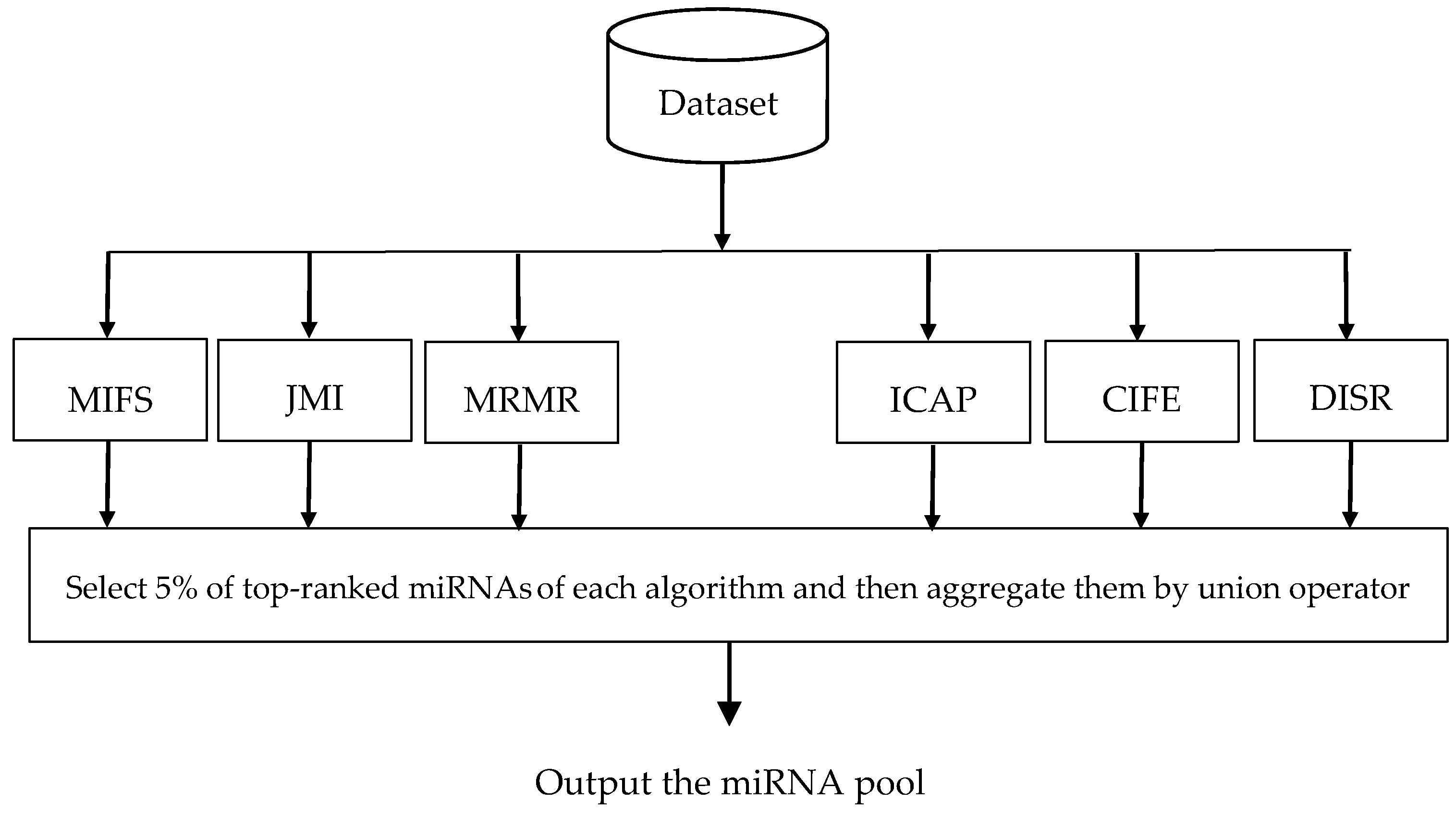
In this paper, we use six filter algorithms to construct miRNA pool, including Mutual Information Feature Selection (MIFS) [41], Joint Mutual Information (JMI) [42], Max-Relevance Min-Redundancy (MRMR) [43], Interaction Capping (ICAP) [44], Conditional Infomax Feature Extraction (CIFE) [45], and Double Input Symmetrical Relevance (DISR) [46]. Figure 1 illustrates the flowchart of miRNA pool generation. As can be seen in this figure, at first some ranking lists are generated using different filter algorithms, then 5% of top-ranked miRNAs of each ranking list is extracted, and finally, all of the extracted top-ranked miRNAs are integrated using the well-known union operator.
3.2. Weighting the miRNAs of miRNA Pool
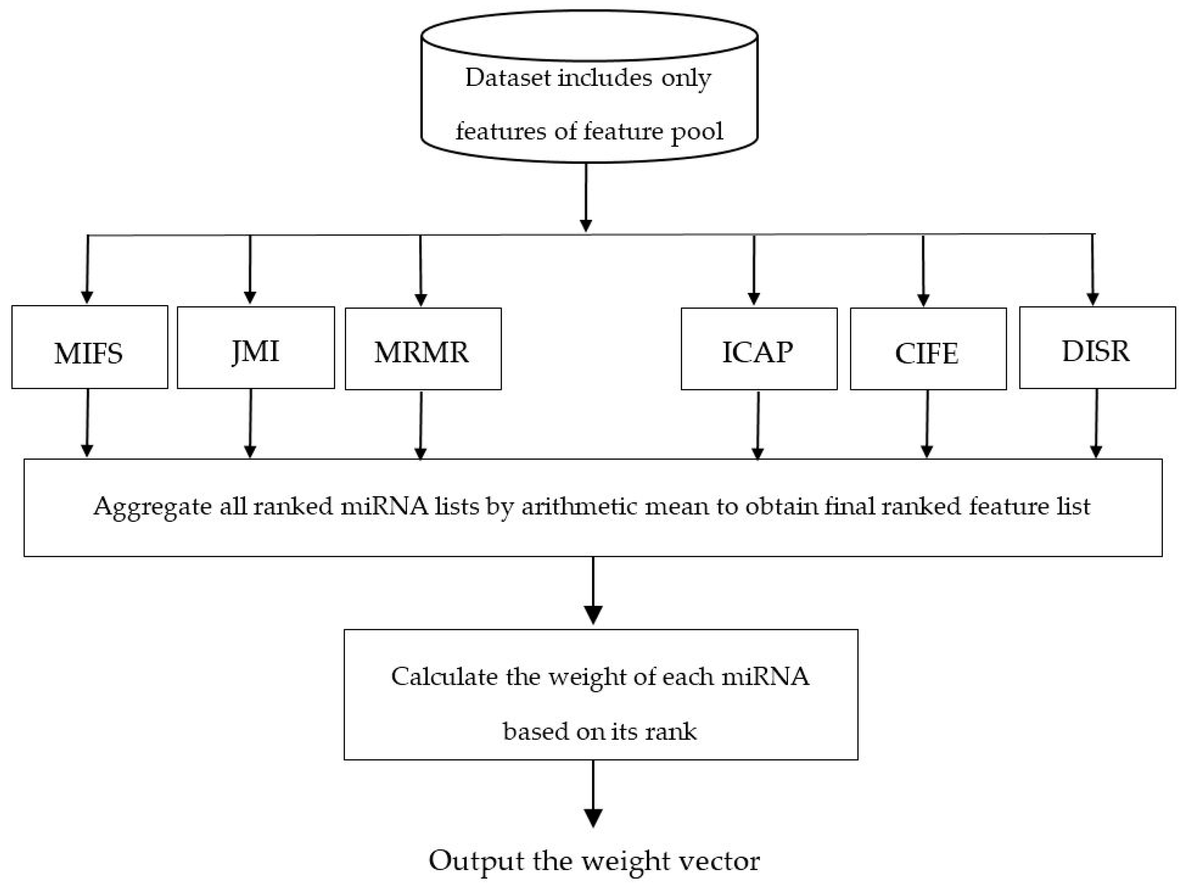
Figure 2 illustrates the flowchart of calculating the weight vector for features of the dataset. As can be seen in this figure, some ranking lists are generated using different filter-based algorithms for miRNA ranking and then these different ranking lists are integrated by the well-known arithmetic mean, where the final score of feature d is calculated by the mean of the ranking scores of this miRNAs in each ranking list. To calculate the weight vector, we normalize the final miRNA ranking vector obtained between 0.01 and 0.2 using min-max normalization method [47].
3.3. Solution Representation
To design a metaheuristic, representation is necessary to encode each solution of the problem. The representation used in the proposed algorithm is the well-known real-valued representation. During the execution of the algorithm, all particles are allowed to have a real value between [0, 1]. It should be noted that the algorithm performs the entire search operation in continues space. Therefore, to solve miRNA subset selection problem with proposed algorithm a threshold parameter is needed to map solutions in continuous space to solutions in binary (miRNA) space. This threshold parameter is obtained weight vector described in the previous section.
3.4. Fuzzy Balancer to Balance between Exploration and Exploitation
In this section, we propose a fuzzy inference system to intelligently manage the balance between exploration and exploitation by adjusting the value of [48,49,50,51]. For this purpose, a zero-order T–S fuzzy inference system with two inputs and one output is used [52]. Two inputs for the proposed fuzzy inference system are the normalized current iteration of the algorithm and the normalized diversity of swarm in decision space. The reason for selecting the current iteration as first input is clear: each algorithm must explore the search space with a diverse swarm at the beginning and change into convergence by lapse of iterations. In this paper, the normalized current iteration is calculated for fuzzy balancer as follows:
where t is the number of iterations elapsed and T is the maximal number of iterations. It is necessary to mention that iter is equal to “0” if algorithm is in the first iteration, is equal to “1” if algorithm is in the last iteration, and in general we have .
The main reason for selecting the diversity of swarm as a second input of fuzzy balancer is that whatever the swarm diversity is, we have good exploration and it does not require more exploration. In this paper, we propose a new equation to calculate the diversity as follows:
where N is the number of particles, n is the number of miRNAs, and is the variance between all particles in dimension d. It is noteworthy that diversity is equal to “0” if all particles converge to a single solution, is equal to “1” if for each dimension of all particles we have in which is the upper bound on the variance of each variable that takes on values in range [0, 1] (Note that we can calculate the upper bound on the variance of each variable which takes its values in range [a, b] by ) [53]. Therefore, in general we have 0 ≤ diversity ≤ 1.
The output of the proposed fuzzy inference system is the value of , because the exploration ability of proposed algorithm depends on the its value. As we know, a larger value of this parameter encourages exploration, while a smaller value of it provides exploitation. Using these facts, the following rule-base is proposed to calculate the value of by fuzzy inference system:
- If iter is Low and diversity is Low, then = VHigh.
- If iter is Low and diversity is Med, then = High.
- If iter is Low and diversity is High, then = Med.
- If iter is Med and diversity is Low, then = High.
- If iter is Med and diversity is Med, then = Med.
- If iter is Med and diversity is High, then = Low.
- If iter is High and diversity is Low, then = Med.
- If iter is High and diversity is Med, then = Low.
- If iter is High and diversity is High, then = VLow.
For partitioning the input spaces of iter and diversity variables, we use a general rule where the resulting fuzzy term sets for both variables are orthogonal with -completeness equal to 0.5. Figure 3 shows the input membership functions of the proposed fuzzy inference system. The rule’s consequences are set as: VHigh = 1, High = 0.5, Med = 0.2, Low = 0.1, and VLow = 0.01.
3.5. Particle Evaluation
Each metaheuristic must use a fitness (or cost) evaluation function which associates with each solution of the search space a numeric value that describes its quality. An effective fitness (cost) evaluation function must yield better evaluations to solutions that are closer to the optimal solution than those that are farther away.
To evaluate the cost of the miRNAs subset selection and avoid the over-fitting, we use the average error rates of n-fold cross-validation (with n = 10) on training data. In this case, we use the k-Nearest Neighbors (k-NN) classifier [54] with k = 5 as learning algorithm for wrapper. The k-NN is a type of instance-based machine learning algorithm where its input is the k training instances in the miRNAs space and its output is a class label. In k-NN, an instance is labeled by the majority class of its k nearest neighbors.
3.6. Algorithmic Details and Flowchart
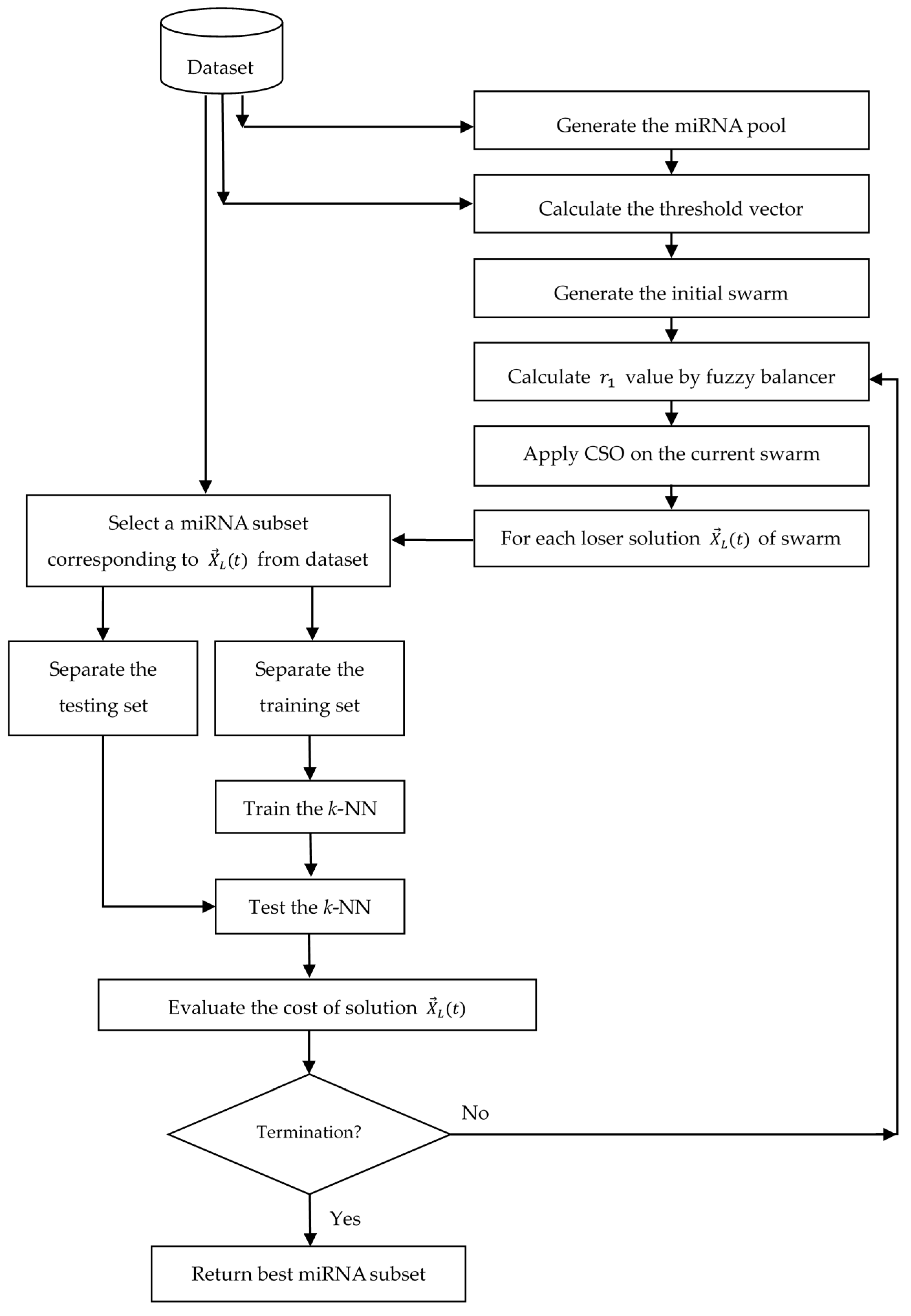
Algorithm 2 shows the detailed algorithmic steps of proposed algorithm, and Figure 4 illustrates the system architecture of it. Algorithm 3 shows the general steps of n-fold cross-validation.
| Algorithm 2. Outline of proposed algorithm for feature selection in classification. |
| // first stage: miRNA pool generation |
| Calculate the rank of each miRNA by every filter algorithms; |
| Construct miRNA pool by high-ranked miRNAs; |
| // second stage: miRNA weights calculation |
| Calculate the rank of each miRNA of miRNA pool by every filter algorithms; |
| Calculate the miRNA weights for each member of miRNA pool and threshold vector |
| ; |
| // third stage: search to find the best miRNA subset of miRNA pool |
| t = 0; |
| For i = 1 to N Do |
| Randomly generate the initial solution ; |
| Randomly generate the initial velocity ; |
| End for |
| While stopping criteria is not satisfied Do |
| ; |
| While Do |
| Randomly choose two different particles and from ; |
| /* algorithmic steps of is shown in Algorithm (3) */ |
| If |
| ; |
| ; |
| Else |
| ; |
| ; |
| End if |
| For each dimension d of update by Eq. (3); |
| For each dimension d of update by Eq. (4); |
| ; |
| ; |
| End while |
| t = t + 1; |
| End while |
| Output: Best solution found. |
| Algorithm 3. Outline of algorithm. |
| Inputs: vector and vector . |
| ; |
| For d = 1 to n Do |
| If |
| ; |
| End if |
| End for |
| Cost = the cost of k-NN by 10-fold cross-validation; |
| Output: Cost of . |
4. Experimental Study
In this section, the effectiveness of the proposed algorithm on the high-dimensional miRNA subset selection problem is evaluated in terms of both the error rate of the k-NN classification and minimizing the number of miRNAs. In the following, we first present the characteristics of the selected datasets and experimental settings. Then, numerical results from the implementation of the proposed algorithm are presented and compared with the results obtained by other several miRNA subset selection algorithms.
4.1. Dataset Properties and Experimental Settings
To evaluate the numerical performance of the proposed algorithm, we conducted several experiments on three cancer datasets, i.e., lung, nasopharyngeal, and melanoma. Table 1 lists the main properties of these datasets. It should be noted that all of these datasets are publicly available and can be easily downloaded from the gene expression omnibus (GEO) [55]. No preprocessing has been performed on datasets. For each dataset, training data is randomly generated with 70% instances being used as the dataset, and the remaining instances are considered as testing set.
In the comparison, 17 algorithms are implemented and tested on Matlab 2015b, all based on the well-known k-NN classifier with k = 5. To show the performance of the proposed algorithm, we compare it with the standard GA, the original CSO algorithm [25], the original PSO, DE [32], ABC-DE [34], ACO-FS [31], ACO-ABC [33], GSA [56], BQIGSA [57], four variants of PSO proposed by Xue’s for bi-objective feature subset selection [36] (Xue1-PSO, Xue2-PSO, Xue3-PSO, and Xue4-PSO), and three two-stage algorithms include 2S-GA [40], 2S-HGA [41], and 2S-PSO [39]. Based on Xue et al. [36], the major difference between Xue’s algorithms is the number of features selected in the initial swarm, while Xue1-PSO uses the normal initialization method where approximately half of the features are chosen in each particles, Xue2-PSO applies a little initialization method in which only about 10% features are chosen in each particles, Xue3-PSO applies heavy initialization method in which more than half (about 2/3) of the features are chosen in each particles, and Xue4-PSO applies a combined initialization in which a major (about 2/3) of the particles are initialized with the little initialization method, while the remaining particles of swarm are initialized with the heavy initialization method. Another important difference between Xue’s algorithms and canonical PSO-based algorithms is that in Xue’s algorithm, the threshold parameter λ is set to 0.6, while this parameter is set to 0.5 as the threshold parameter in canonical PSO.
The population or swarm size is set to 100 for all metaheuristics, and the maximum number of fitness evaluation is set to 20,000. Other parameters of some algorithms are: w in the PSO is set to 0.7298, both c1 and c2 in the PSO are set to 1.49618. The particles in all algorithms are randomly initialized and the threshold parameter λ = 0.5 is used for the original PSO, while λ = 0.6 is used for Xue’s algorithms. Also, the experimental settings of other algorithms are adopted exactly as in their original works. To obtain statistical results, each algorithm is run for 30 times independently.
4.2. Results and Comparisons
Although there are several criteria for assessing the quality of a classifier, however, the main goal of a classifier is to improve the generalization capability, which means a high accuracy or low misclassification rate on the unseen data. Therefore, here we are going to obtain the average error rate or misclassification rate of all the compared feature subset selection algorithms. The generated results by all feature subset selection algorithms are presented in Table 2. We also apply the statistical Wilcoxon rank sum test [58] to compare the results of the proposed algorithm and other compared algorithms for feature subset selection. The result is also listed in Table 2, where the symbols “+”, “≈”, and “−” represent that other methods are statistically inferior to, equal to, or superior to the proposed algorithm, respectively. The average positive predictive value of different algorithms is presented in Table 3.
The experimental results show that the proposed algorithm has a lower statistical misclassification rate than other compared miRNA subset selection algorithms on all benchmark datasets. The main reason for the superiority of the proposed algorithm is that this algorithm removes lowly-ranked miRNAs from the search process and weight top-ranked miRNAs.
The removing all irrelevant and redundant miRNAs to improve the classifier is the second goal of miRNAs subset selection problem. Therefore, we also look at the statistical number of chosen miRNAs generated by the compared miRNAs subset selection algorithms. The obtained results are listed in Table 4. In this comparison, it is visible that the proposed algorithm chooses fewer average miRNAs than most compared algorithms. The main reason for this superiority is that the irrelevant miRNAs have a little chance of being selected, and many of them are not selected during the search due to their inefficiencies in classification. From Table 4, it is visible that the number of miRNAs chosen by the PSO-based algorithms are proportional to the number of miRNAs initialized in the first generation. In other words, if we initialize the particles of swarm with a small number of miRNAs, the number of miRNAs chosen in the final swarm will be smaller and vice versa. By contrast, the proposed algorithm is not sensitive to the number of miRNAs initialized in the first iteration, which can always find the near-optimal miRNA subset regardless the number of miRNAs chosen during the particle initialization phase. Given that the proposed algorithm is a randomized algorithm, different miRNAs may be selected in each replication. Therefore, the most frequently selected miRNAs by the proposed algorithm are given in Table 5.
To understand the effect of ensembling the filter algorithms, a comparison is made between the proposed algorithm and the filter algorithms individually. The results of these experiments are presented in Table 6. As can be seen in this table, ensembling the filter algorithms often improves the results.
5. Conclusions and Future Work
To solve the miRNA subset selection problem with continuous optimization algorithms, a threshold parameter is needed to map solutions in continuous space to solutions in binary (miRNA) space. In all previous continuous optimization algorithms, the threshold parameter is set with the same value for all features. This causes the algorithm to not distinguish between relevant and irrelevant miRNAs, and therefore requires significant time to find optimal miRNAs subsets. This paper tries to increase the cancer classification accuracy by a novel three-stage framework. In the first stage of the proposed framework, multiple filter algorithms are used for ranking the miRNAs according to their relevance with the class label, and generating a miRNA pool obtained based on the top-ranked miRNAs of each filter algorithm. In the second stage, we rank the miRNAs of the miRNA pool by multiple filter algorithms and then this ranking is used to weight the probability of selecting each miRNA. In the third stage, Competitive Swarm Optimization (CSO) tries to find an optimal subset from the weighed miRNAs of the miRNA pool, which gives us the most information about cancer. Experiments on several high-dimensional datasets indicate that using the importance of miRNAs to adjust threshold parameters in CSO has a great performance in terms of both the error rate of the cancer classification and minimizing the number of miRNAs.
For future research, the proposed three-stage framework can be studied on other continuous optimization algorithms such as Artificial Bee Colony (ABC), Deferential Evolution Algorithm (DEA), and so on. Also, the effectiveness of the proposed algorithm for solving the multi-objective feature subset selection and multimodal feature subset selection can be investigated. Finally, one can research how to use the three-stage framework to help other operators of an optimization algorithm. If you have a requirement that you don’t see on the paper or if you have questions, please send an email to [email protected].
Acknowledgments
The authors would like to acknowledge the constructive comments and suggestions of the anonymous referees.
Author Contributions
Mohammad Bagher Dowlatshahi, Vali Derhami, and Hossein Nezamabadi-pour proposed the research idea, then Mohammad Bagher Dowlatshahi implemented the experiments, and finally Mohammad Bagher Dowlatshahi and Vali Derhami wrote the manuscript. All authors discussed the results and contributed to the final manuscript.
Conflicts of Interest
The authors declare no conflict of interest.
References
- Chandrashekar, G.; Sahin, F. A survey on feature selection methods. Comput. Electr. Eng. 2014, 40, 16–28. [Google Scholar] [CrossRef]
- Gheyas, I.A.; Smith, L.S. Feature subset selection in large dimensionality domains. Pattern Recognit. 2010, 43, 5–13. [Google Scholar] [CrossRef]
- Garey, M.R.; Johnson, D.S. A Guide to the Theory of NP-Completeness, 1st ed.; WH Freemann: New York, NY, USA, 1979; ISBN 978-0716710455. [Google Scholar]
- Xue, B.; Zhang, M.; Browne, W.N.; Yao, X. A survey on evolutionary computation approaches to feature selection. IEEE. Trans. Evolut. Comput. 2016, 20, 606–626. [Google Scholar] [CrossRef]
- Pudil, P.; Novovičová, J.; Kittler, J. Floating search methods in feature selection. Pattern Recogn. Lett. 1994, 15, 1119–1125. [Google Scholar] [CrossRef]
- Alpaydin, E. Introduction to Machine Learning, 3rd ed.; MIT Press: Cambridge, MA, USA, 2014; ISBN 978-8120350786. [Google Scholar]
- Talbi, E.G. Metaheuristics: From Design to Implementation; John Wiley & Sons: Hoboken, NJ, USA, 2009; ISBN 978-0470278581. [Google Scholar]
- Dowlatshahi, M.B.; Nezamabadi-Pour, H.; Mashinchi, M. A discrete gravitational search algorithm for solving combinatorial optimization problems. Inf. Sci. 2014, 258, 94–107. [Google Scholar] [CrossRef]
- Han, K.H.; Kim, J.H. Quantum-inspired evolutionary algorithm for a class of combinatorial optimization. IEEE. Trans. Evolut. Comput. 2002, 6, 580–593. [Google Scholar] [CrossRef]
- Banks, A.; Vincent, J.; Anyakoha, C. A review of particle swarm optimization. Part II: hybridisation, combinatorial, multicriteria and constrained optimization, and indicative applications. Nat. Comput. 2008, 7, 109–124. [Google Scholar] [CrossRef]
- Cheng, R.; Jin, Y. A competitive swarm optimizer for large scale optimization. IEEE. Trans. Cybern. 2015, 45, 191–204. [Google Scholar] [CrossRef] [PubMed]
- Dowlatshahi, M.B.; Rezaeian, M. Training spiking neurons with gravitational search algorithm for data classification. In Proceedings of the Swarm Intelligence and Evolutionary Computation (CSIEC), Bam, Iran, 9–11 March 2016; pp. 53–58. [Google Scholar]
- Dowlatshahi, M.B.; Derhami, V. Winner Determination in Combinatorial Auctions using Hybrid Ant Colony Optimization and Multi-Neighborhood Local Search. J. AI Data Min. 2017, 5, 169–181. [Google Scholar]
- Xue, B.; Zhang, M.; Browne, W.N. Multi-objective particle swarm optimisation (PSO) for feature selection. In Proceedings of the 14th Annual Conference on Genetic and Evolutionary Computation Conference (GECCO), Philadelphia, PA, USA, 7–11 July 2012; pp. 81–88. [Google Scholar]
- Zhang, Y.; Gong, D.W.; Cheng, J. Multi-objective particle swarm optimization approach for cost-based feature selection in classification. IEEE/ACM. Trans. Comput. Biol. Bioinform. 2017, 14, 64–75. [Google Scholar] [CrossRef] [PubMed]
- Siedlecki, W.; Sklansky, J. A note on genetic algorithms for large-scale feature selection. Pattern Recogn. Lett. 1989, 10, 335–347. [Google Scholar] [CrossRef]
- Li, Y.; Zhang, S.; Zeng, X. Research of multi-population agent genetic algorithm for feature selection. Expert. Syst. Appl. 2009, 36, 11570–11581. [Google Scholar] [CrossRef]
- Kabir, M.M.; Shahjahan, M.; Murase, K. A new local search based hybrid genetic algorithm for feature selection. Neurocomputing 2011, 74, 2914–2928. [Google Scholar] [CrossRef]
- Eroglu, D.Y.; Kilic, K. A novel Hybrid Genetic Local Search Algorithm for feature selection and weighting with an application in strategic decision making in innovation management. Inf. Sci. 2017, 405, 18–32. [Google Scholar] [CrossRef]
- Phan, A.V.; Le Nguyen, M.; Bui, L.T. Feature weighting and SVM parameters optimization based on genetic algorithms for classification problems. Appl. Intell. 2017, 46, 455–469. [Google Scholar] [CrossRef]
- Derrac, J.; Garcia, S.; Herrera, F. A first study on the use of coevolutionary algorithms for instance and feature selection. Hybrid Artif. Intell. Syst. 2009, 5572, 557–564. [Google Scholar]
- Oh, I.; Lee, J.S.; Moon, B.R. Hybrid genetic algorithm for feature selection. IEEE. Trans. Pattern Anal. Mach. Intell. 2004, 26, 1424–1437. [Google Scholar] [PubMed]
- Huang, C.L.; Dun, J.F. A distributed PSO–SVM hybrid system with feature selection and parameter optimization. Appl. Soft. Comput. 2008, 8, 1381–1391. [Google Scholar] [CrossRef]
- Chuang, L.Y.; Yang, C.H.; Li, J.C. Chaotic maps based on binary particle swarm optimization for feature selection. Appl. Soft. Comput. 2011, 11, 239–248. [Google Scholar] [CrossRef]
- Gu, S.; Cheng, R.; Jin, Y. Feature selection for high-dimensional classification using a competitive swarm optimizer. Soft Comput. 2016, 1–12. [Google Scholar] [CrossRef]
- Wei, J.; Zhang, R.; Yu, Z.; Hu, R.; Tang, J.; Gui, C.; Yuan, Y. A BPSO-SVM algorithm based on memory renewal and enhanced mutation mechanisms for feature selection. Appl. Soft. Comput. 2017, 58, 176–192. [Google Scholar] [CrossRef]
- Bello, R.; Gomez, Y.; Garcia, M.M.; Nowe, A. Two-step particle swarm optimization to solve the feature selection problem. In Proceedings of the Seventh International Conference on Intelligent Systems Design and Applications (ISDA 2007), Rio de Janeiro, Brazil, 20–24 October 2007; pp. 691–696. [Google Scholar]
- Tanaka, K.; Kurita, T.; Kawabe, T. Selection of import vectors via binary particle swarm optimization and cross-validation for kernel logistic regression. In Proceedings of the 2007 International Joint Conference on Neural Networks, Orlando, FL, USA, 12–17 August 2007; pp. 12–17. [Google Scholar]
- Wang, X.; Yang, J.; Teng, X.; Xia, W.; Jensen, R. Feature selection based on rough sets and particle swarm optimization. Pattern Recognit. Lett. 2007, 28, 459–471. [Google Scholar] [CrossRef] [Green Version]
- Sivagaminathan, R.K.; Ramakrishnan, S. A hybrid approach for feature subset selection using neural networks and ant colony optimization. Expert. Syst. Appl. 2007, 33, 49–60. [Google Scholar] [CrossRef]
- Kashef, S.; Nezamabadi-pour, H. An advanced ACO algorithm for feature subset selection. Neurocomputing 2014, 147, 271–279. [Google Scholar] [CrossRef]
- Ghosh, A.; Datta, A.; Ghosh, S. Self-adaptive differential evolution for feature selection in hyperspectral image data. Appl. Soft. Comput. 2013, 3, 1969–1977. [Google Scholar] [CrossRef]
- Shunmugapriya, P.; Kanmani, S. A hybrid algorithm using ant and bee colony optimization for feature selection and classification (AC-ABC Hybrid). Swarm Evol. Comput. 2017, 36, 27–36. [Google Scholar] [CrossRef]
- Zorarpacı, E.; Özel, S.A. A hybrid approach of differential evolution and artificial bee colony for feature selection. Expert Syst. Appl. 2016, 62, 91–103. [Google Scholar] [CrossRef]
- Vieira, S.; Sousa, J.; Runkler, T. Multi-criteria ant feature selection using fuzzy classifiers. In Swarm Intelligence for Multi-objective Problems in Data Mining, vol. 242 of Studies in Computational Intelligence; Springer: Berlin, Germany, 2009; pp. 19–36. [Google Scholar]
- Xue, B.; Zhang, M.; Browne, W.N. Particle swarm optimization for feature selection in classification: A multi-objective approach. IEEE. Trans. Cybern. 2013, 43, 1656–1671. [Google Scholar] [CrossRef] [PubMed]
- Xue, B.; Fu, W.; Zhang, M. Multi-objective feature selection in classification: A differential evolution approach. In Proceedings of the Asia-Pacific Conference on Simulated Evolution and Learning, Dunedin, New Zealand, 15–18 December 2014; pp. 516–528. [Google Scholar]
- Sahu, B.; Mishra, D. A novel feature selection algorithm using particle swarm optimization for cancer microarray data. Procedia Eng. 2012, 38, 27–31. [Google Scholar] [CrossRef]
- Oreski, S.; Oreski, G. Genetic algorithm-based heuristic for feature selection in credit risk assessment. Expert. Syst. Appl. 2014, 41, 2052–2064. [Google Scholar] [CrossRef]
- Tan, F.; Fu, X.Z.; Zhang, Y.Q.; Bourgeois, A. A genetic algorithm based method for feature subset selection. Soft Comput. 2008, 12, 111–120. [Google Scholar] [CrossRef]
- Battiti, R. Using mutual information for selecting features in supervised neural net learning. IEEE. Trans. Neural Netw. 1994, 5, 537–550. [Google Scholar] [CrossRef] [PubMed]
- Yang, H.; Moody, J. Data visualization and feature selection: New algorithms for non-gaussian data. In Advances in Neural Information Processing Systems; MIT Press: Cambridge, MA, USA, 1999; pp. 687–693. [Google Scholar]
- Peng, H.; Long, F.; Ding, C. Feature selection based on mutual information: Criteria of max-dependency, max-relevance, and min-redundancy. IEEE. Trans. Pattern Anal. Mach. Intell. 2005, 27, 1226–1238. [Google Scholar] [CrossRef] [PubMed]
- Jakulin, A. Machine Learning Based on Attribute Interactions. Ph.D. Thesis, University of Ljubljana, Ljubljana, Slovenia, 2005. [Google Scholar]
- Lin, D.; Tang, X. Conditional infomax learning: An integrated framework for feature extraction and fusion. In Proceedings of the 9th European Conference on Computer Vision, Graz, Austria, 7–13 May 2006; pp. 68–82. [Google Scholar]
- Meyer, P.; Bontempi, G. On the use of variable complementarity for feature selection in cancer classification. In Proceedings of the Evolutionary Computation and Machine Learning in Bioinformatics, Budapest, Hungary, 10–12 April 2006; pp. 91–102. [Google Scholar]
- Han, J.; Pei, J.; Kamber, M. Data Mining: Concepts and Techniques, 3rd ed.; Elsevier: Amsterdam, The Netherlands, 2011; ISBN 978-9380931913. [Google Scholar]
- Dowlatshahi, M.B.; Nezamabadi-Pour, H. GGSA: a grouping gravitational search algorithm for data clustering. Eng. Appl. Artif. Intell. 2014, 36, 114–121. [Google Scholar] [CrossRef]
- Črepinšek, M.; Liu, S.H.; Mernik, M. Exploration and exploitation in evolutionary algorithms: A survey. ACM Comput. Surv. 2013, 45, 1–35. [Google Scholar] [CrossRef]
- Rafsanjani, M.K.; Dowlatshahi, M.B. A Gravitational search algorithm for finding near-optimal base station location in two-tiered WSNs. In Proceedings of the 3rd International Conference on Machine Learning and Computing, Singapore, 26–28 February 2011; pp. 213–216. [Google Scholar]
- Dowlatshahi, M.B.; Derhami, V.; Nezamabadi-pour, H. Ensemble of Filter-Based Rankers to Guide an Epsilon-Greedy Swarm Optimizer for High-Dimensional Feature Subset Selection. Information 2017, 8, 152. [Google Scholar] [CrossRef]
- Li, H.; Wang, J.; Du, H.; Karimi, H.R. Adaptive sliding mode control for Takagi-Sugeno fuzzy systems and its applications. IEEE. Trans. Fuzzy Syst. 2017, in press. [Google Scholar] [CrossRef]
- Van Blerkom, M.L. Measurement and Statistics for Teachers; Taylor & Francis: Didcot, UK, 2017. [Google Scholar]
- Abbasifard, M.R.; Ghahremani, B.; Naderi, H. A survey on nearest neighbor search methods. Int. J. Comput. Appl. 2014, 95, 39–52. [Google Scholar]
- Gene Expression Omnibus (GEO). Available online: https://www.ncbi.nlm.nih.gov/geo/ (accessed on 19 October 2017).
- Han, X.; Chang, X.; Quan, L.; Xiong, X.; Li, J.; Zhang, Z.; Liu, Y. Feature subset selection by gravitational search algorithm optimization. Inf. Sci. 2014, 281, 128–146. [Google Scholar] [CrossRef]
- Barani, F.; Mirhosseini, M.; Nezamabadi-pour, H. Application of binary quantum-inspired gravitational search algorithm in feature subset selection. Appl. Intell. 2017, 47, 304–318. [Google Scholar] [CrossRef]
- Derrac, J.; García, S.; Molina, D.; Herrera, F. A practical tutorial on the use of nonparametric statistical tests as a methodology for comparing evolutionary and swarm intelligence algorithms. Swarm Evol. Comput. 2011, 1, 3–18. [Google Scholar] [CrossRef]
Figure 1.
Flowchart of the ensemble of filter algorithms to generate the Micro-Ribonucleic Acids (miRNA) pool.
Figure 1.
Flowchart of the ensemble of filter algorithms to generate the Micro-Ribonucleic Acids (miRNA) pool.

Figure 2.
Flowchart of the ensemble of filter algorithms to calculate the weight vector.

Figure 3.
Input membership functions of the proposed fuzzy inference system.
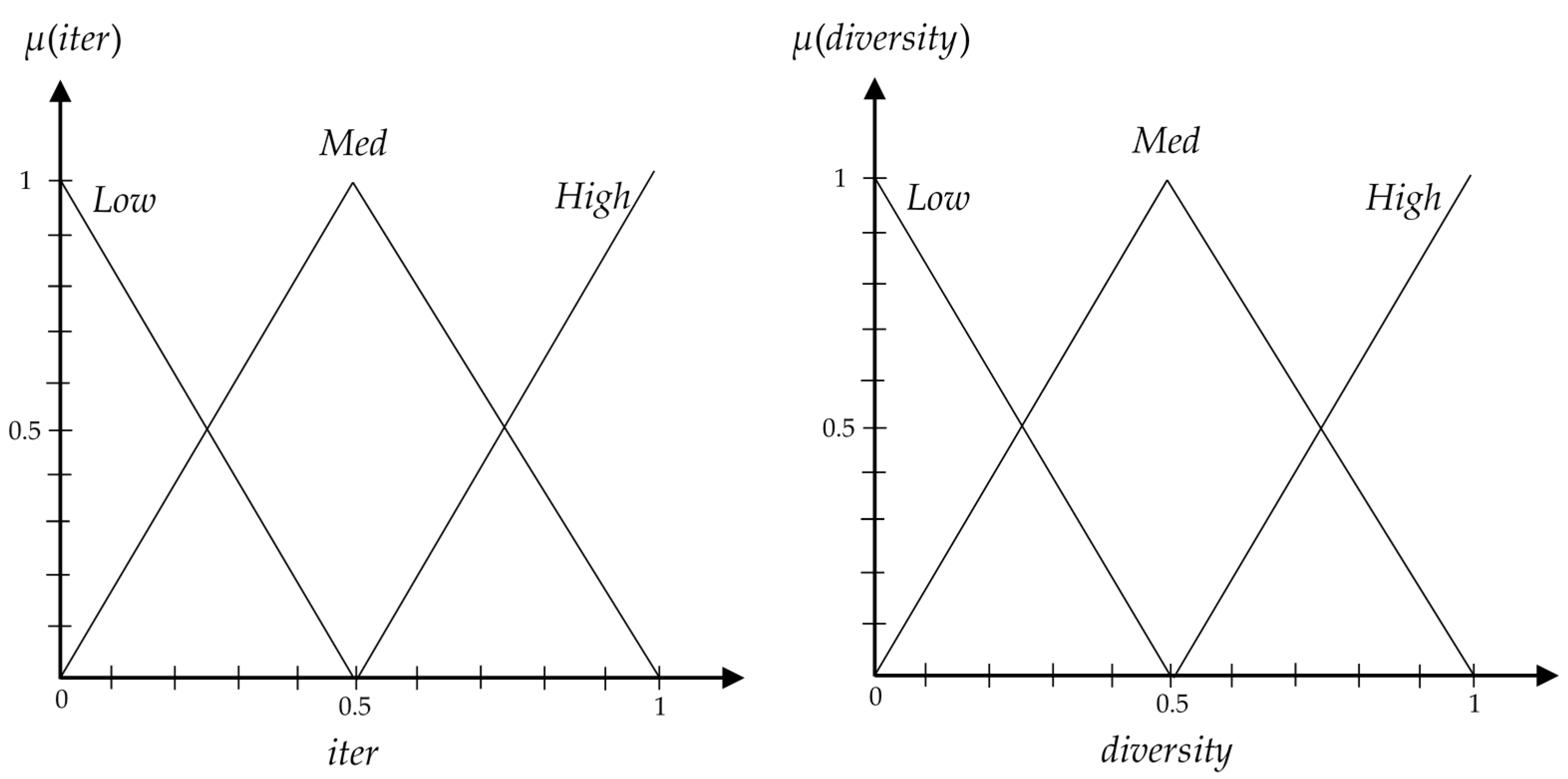
Figure 4.
System architecture of the proposed algorithm for miRNA subset selection.


Table 1.
The main properties of benchmark datasets.
| Dataset | No. of miRNAs | No. of Normal Patients | No. of Cancer Patients | No. of Classes |
|---|---|---|---|---|
| Lung | 866 | 19 | 17 | 2 |
| Nasopharyngeal | 887 | 19 | 31 | 2 |
| Melanoma | 864 | 22 | 35 | 2 |
Table 2.
Average error rate of different algorithms in cancer classification.
| Dataset | Lung | Nasopharyngeal | Melanoma |
|---|---|---|---|
| Proposed algorithm | 0.1931 | 0.3257 | 0.1605 |
| (0.0159) | (0.0317) | (0.0179) | |
| GA | 0.3312 + | 0.4623 + | 0.2981 + |
| (0.0393) | (0.0396) | (0.0296) | |
| CSO | 0.2607 + | 0.3393 ≈ | 0.2350 + |
| (0.0236) | (0.0352) | (0.0284) | |
| PSO | 0.3515 + | 0.4625 + | 0.3173 + |
| (0.0442) | (0.0342) | (0.0342) | |
| DE | 0.3227 + | 0.3902 + | 0.3092 + |
| (0.0371) | (0.0325) | (0.0307) | |
| ABC-DE | 0.3073 + | 0.3721 + | 0.3217 + |
| (0.0481) | (0.0362) | (0.0374) | |
| ACOFS | 0.3406 + | 0.3916 + | 0.3686 + |
| (0.0361) | (0.0403) | (0.0391) | |
| ACO-ABC | 0.3204 + | 0.3993 + | 0.2730 + |
| (0.0382) | (0.0381) | (0.0311) | |
| GSA | 0.3372 + | 0.3931 + | 0.3511 + |
| (0.0423) | (0.0350) | (0.0368) | |
| BQIGSA | 0.3007 + | 0.3384 ≈ | 0.2761 + |
| (0.0299) | (0.0301) | (0.0273) | |
| Xue1-PSO | 0.3603 + | 0.4321 + | 0.3154 + |
| (0.0490) | (0.0314) | (0.0491) | |
| Xue2-PSO | 0.3249 + | 0.3791 + | 0.2920 + |
| (0.0405) | (0.0424) | (0.0301) | |
| Xue3-PSO | 0.3618 + | 0.4412 + | 0.3064 + |
| (0.0506) | (0.0376) | (0.0429) | |
| Xue4-PSO | 0.3242 + | 0.3918 + | 0.2796 + |
| (0.0345) | (0.0350) | (0.0307) | |
| 2S-GA | 0.2785 + | 0.3341 ≈ | 0.2532 + |
| (0.0272) | (0.0366) | (0.0291) | |
| 2S-HGA | 0.2804 + | 0.3393 ≈ | 0.2699 + |
| (0.0316) | (0.0348) | (0.0254) | |
| 2S-PSO | 0.2523 + | 0.3478 + | 0.2382 + |
| (0.0205) | (0.0351) | (0.0232) | |
| Better | 16 | 13 | 16 |
| Worse | 0 | 0 | 0 |
| Similar | 0 | 3 | 0 |
The symbols “+”, “≈”, and “−” represent that other methods are statistically inferior to, equal to, or superior to the proposed algorithm, respectively.
Table 3.
Average positive predictive value of different algorithms in cancer classification.
| Dataset | Lung | Nasopharyngeal | Melanoma |
|---|---|---|---|
| Proposed algorithm | 0.8852 | 0.6949 | 0.9217 |
| (0.0317) | (0.0317) | (0.0253) | |
| GA | 0.7021 + | 0.5731 + | 0.7326 + |
| (0.0437) | (0.0482) | (0.0491) | |
| CSO | 0.7419 + | 0.5874 + | 0.7147 + |
| (0.0379) | (0.0391) | (0.0572) | |
| PSO | 0.7112 + | 0.5730 + | 0.7492 + |
| (0.0512) | (0.0462) | (0.0420) | |
| DE | 0.6826 + | 0.5592 + | 0.7718 + |
| (0.0417) | (0.0418) | (0.0325) | |
| ABC-DE | 0.6991 + | 0.5973 + | 0.7930 + |
| (0.0454) | (0.0427) | (0.0458) | |
| ACOFS | 0.6592 + | 0.6881 ≈ | 0.7504 + |
| (0.0459) | (0.0425) | (0.0429) | |
| ACO-ABC | 0.6811 + | 0.5347 + | 0.8271 + |
| (0.0357) | (0.0452) | (0.0342) | |
| GSA | 0.6927 + | 0.5696 + | 0.7906 + |
| (0.0448) | (0.0406) | (0.0394) | |
| BQIGSA | 0.7284 + | 0.5872 + | 0.8985 ≈ |
| (0.0521) | (0.0397) | (0.0294) | |
| Xue1-PSO | 0.6268 + | 0.5303 + | 0.7892 + |
| (0.0457) | (0.0472) | (0.0426) | |
| Xue2-PSO | 0.6995 + | 0.5605 + | 0.8427 + |
| (0.0452) | (0.0403) | (0.0368) | |
| Xue3-PSO | 0.6817 + | 0.5482 + | 0.8244 + |
| (0.0481) | (0.0495) | (0.0401) | |
| Xue4-PSO | 0.7393 + | 0.5881 + | 0.8625 + |
| (0.0479) | (0.0573) | (0.0429) | |
| 2S-GA | 0.7692 + | 0.6822 ≈ | 0.8751 + |
| (0.0472) | (0.0415) | (0.0284) | |
| 2S-HGA | 0.7824 + | 0.6798 ≈ | 0.8901 + |
| (0.0385) | (0.0381) | (0.0372) | |
| 2S-PSO | 0.7924 + | 0.6402 + | 0.9063 ≈ |
| (0.0322) | (0.0493) | (0.0371) | |
| Better | 16 | 13 | 16 |
| Worse | 0 | 0 | 0 |
| Similar | 0 | 3 | 2 |
The symbols “+”, “≈”, and “−” represent that other methods are statistically inferior to, equal to, or superior to the proposed algorithm, respectively.
Table 4.
Average number of selected miRNAs by different algorithms.
| Dataset | Lung | Nasopharyngeal | Melanoma |
|---|---|---|---|
| Proposed algorithm | 9.74 | 15.58 | 15.21 |
| (5.36) | (3.18) | (7.82) | |
| GA | 35.62 + | 292.26 + | 41.65 + |
| (18.52) | (16.02) | (19.23) | |
| CSO | 14.27 + | 15.22 ≈ | 20.52 + |
| (13.43) | (5.41) | (10.29) | |
| PSO | 30.44 + | 267.18 + | 37.93 + |
| (19.17) | (13.36) | (21.16) | |
| DE | 31.15 + | 225.48 + | 35.19 + |
| (15.66) | (12.15) | (18.80) | |
| ABC-DE | 47.91 + | 261.37 + | 42.01 + |
| (20.41) | (13.83) | (21.13) | |
| ACOFS | 50.14 + | 261.31 + | 40.24 + |
| (23.62) | (12.21) | (17.91) | |
| ACO-ABC | 32.81 + | 251.07 + | 36.74 + |
| (19.60) | (14.11) | (19.05) | |
| GSA | 52.83 + | 290.18 + | 41.10 + |
| (25.12) | (16.33) | (24.16) | |
| BQIGSA | 30.05 + | 242.36 + | 37.35 + |
| (17.91) | (15.13) | (16.87) | |
| Xue1-PSO | 29.37 + | 266.31 + | 36.13 + |
| (17.44) | (15.32) | (18.65) | |
| Xue2-PSO | 17.64 + | 31.06 + | 23.18 + |
| (21.49) | (8.42) | (15.75) | |
| Xue3-PSO | 28.14 + | 322.19 + | 34.92 + |
| (19.62) | (26.52) | (16.35) | |
| Xue4-PSO | 24.02 + | 273.21 + | 30.44 + |
| (16.71) | (32.04) | (17.32) | |
| 2S-GA | 15.67 + | 28.21 + | 22.47 + |
| (12.74) | (7.15) | (10.79) | |
| 2S-HGA | 17.05 + | 15.66 ≈ | 24.10 + |
| (14.25) | (5.73) | (12.32) | |
| 2S-PSO | 16.31 + | 23.14 + | 21.52 + |
| (13.27) | (7.35) | (11.26) | |
| Better | 16 | 14 | 16 |
| Worse | 0 | 0 | 0 |
| Similar | 0 | 2 | 0 |
The symbols “+”, “≈”, and “−” represent that other methods are statistically inferior to, equal to, or superior to the proposed algorithm, respectively.
Table 5.
The most frequent selected miRNAs by proposed algorithm.
| Lung | Nasopharyngeal | Melanoma |
|---|---|---|
| hsa-let-7d | hsa-miR-638 | hsa-miR-17 |
| hsa-miR-423-5p | hsa-miR-762 | hsa-miR-664 |
| hsa-let-7f | hsa-miR-1915 | hsa-miR-145 |
| hsa-miR-140-3p | hsa-miR-92a | hsa-miR-422a |
| hsa-miR-25 | hsa-miR-135a | hsa-miR-216a |
| hsa-miR-98 | hsa-miR-181a | hsa-miR-186 |
| hsa-miR-195 | hsa-miR-1275 | hsa-miR-601 |
| hsa-miR-126 | hsa-miR-940 | hsa-miR-1301 |
| hsa-miR-20b | hsa-miR-572 | hsa-miR-328 |
| hsa-let-7e | hsa-miR-29c | hsa-miR-30d |
| hsa-let-7c | hsa-miR-548q | hsa-let-7d |
Table 6.
Average error rate of individual filter algorithms and proposed algorithm.
| Dataset | Lung | Nasopharyngeal | Melanoma |
|---|---|---|---|
| Proposed algorithm | 0.1931 | 0.3257 | 0.1605 |
| 0.0159 | 0.0317 | 0.0179 | |
| MIFS-k-NN | 0.1822 − | 0.3741 + | 0.2173 + |
| 0.0121 | 0.0324 | 0.0198 | |
| JMI-k-NN | 0.2274 + | 0.3499 + | 0.2394 + |
| 0.0213 | 0.0327 | 0.0219 | |
| MRMR-k-NN | 0.2182 + | 0.3807 + | 0.2201 + |
| 0.0195 | 0.0351 | 0.0214 | |
| ICAP-k-NN | 0.2418 + | 0.3305 ≈ | 0.1994 + |
| 0.0269 | 0.0319 | 0.0201 | |
| CIFE-k-NN | 0.2362 + | 0.3677 + | 0.2319 + |
| 0.0275 | 0.0359 | 0.0237 | |
| DISR-k-NN | 0.2479 + | 0.3803 + | 0.2505 + |
| 0.0304 | 0.0381 | 0.0241 | |
| Better | 5 | 5 | 6 |
| Worse | 1 | 0 | 0 |
| Similar | 0 | 1 | 0 |
The symbols “+”, “≈”, and “−” represent that other methods are statistically inferior to, equal to, or superior to the proposed algorithm, respectively.
© 2018 by the authors. Licensee MDPI, Basel, Switzerland. This article is an open access article distributed under the terms and conditions of the Creative Commons Attribution (CC BY) license (http://creativecommons.org/licenses/by/4.0/).
Share and Cite
MDPI and ACS Style
Dowlatshahi, M.B.; Derhami, V.; Nezamabadi-pour, H. A Novel Three-Stage Filter-Wrapper Framework for miRNA Subset Selection in Cancer Classification. Informatics 2018, 5, 13. https://doi.org/10.3390/informatics5010013
AMA Style
Dowlatshahi MB, Derhami V, Nezamabadi-pour H. A Novel Three-Stage Filter-Wrapper Framework for miRNA Subset Selection in Cancer Classification. Informatics. 2018; 5(1):13. https://doi.org/10.3390/informatics5010013
Chicago/Turabian StyleDowlatshahi, Mohammad Bagher, Vali Derhami, and Hossein Nezamabadi-pour. 2018. "A Novel Three-Stage Filter-Wrapper Framework for miRNA Subset Selection in Cancer Classification" Informatics 5, no. 1: 13. https://doi.org/10.3390/informatics5010013
Note that from the first issue of 2016, this journal uses article numbers instead of page numbers. See further details here.