3.1. Plane Waves
We seek standing wave solutions by setting
for
. This gives a set of algebraic equations which can be written in the form of a backwards transfer map
for
independent of
t. Following the procedure in [
18] and for now assuming
, we begin by assuming solutions in the form of plane waves on the linear portions of the chain. That is,
with
representing the incident, reflected and transmitted amplitudes, respectively. The solution Equation (
4) solves Equation (
3) for
only if the wavenumber
k satisfies
. Also directly from Equation (
4) with
we have
The stationary solution across the whole lattice is then known by the following procedure: given values for
for
we start by specifying values for
k and
T. Then we compute
via Equation (
3) and then
by Equation (
5). Such a procedure of finding the input as a function of the output is referred to as a “fixed output problem” [
26].
Stationary solutions where the amplitude
is incident from the right-hand-side and the wavenumber is taken as
can also be formulated in a similar way. In order to avoid swapping the format of Equation (
4) (so that
would apply on the right and
T on left), it is more convenient to leave Equation (
4) as-is with
positive wave number
k and instead flip left-to-right the configuration of the nonlinearities,
i.e.,
. In this way the computation of the solution for negative wavenumber is unchanged from the above outline aside from the swap of the order of the
γ’s. Plots of these plane wave stationary solutions are shown in the next section, where we also address the stability of their
t-propagation. In practice we truncate the lattice and refer to its finite length as
L.
For a solution that has been determined by the processes described above, we next compute the transmission coefficient
explicitly assuming that
T is given. For this purpose it is convenient to write
with
so that
corresponds to
, and incrementing
l corresponds to decreasing
n. In this notation we have
for
and the value of
for each subsequent node towards the left is given by rewriting Equation (
3) as
for
. See the Appendix where we record a few iterations of Equation (
6). Then by Equation (
5) with
computed according to Equation (
6) we have
and
In the linear case () and in the symmetric case ( as an ordered set) it is immediately seen that τ is the same for waves incoming from the left or right side. For the transmission is always symmetric.
We also define here a quantity to measure the asymmetric propagation. We will use the definition of a rectification factor
f in the form of
where the quantity
corresponds to transmission of a left-incoming wave with positive wavenumber
and
with
is equivalent to the transmission of a right-incoming wave with negative wavenumber (recall the process described above of keeping
k positive while flipping the order of the
γ’s). This way nonzero values of
f in the range
measure the asymmetry of transmission in the system. Symmetry in transmission corresponds to
and
corresponds to greater transmission of incident waves originating from the left (transmitted on the right) as compared with incident waves originating from the right (transmitted on the left). Of course,
corresponds to greater transmission of waves originating from the right.
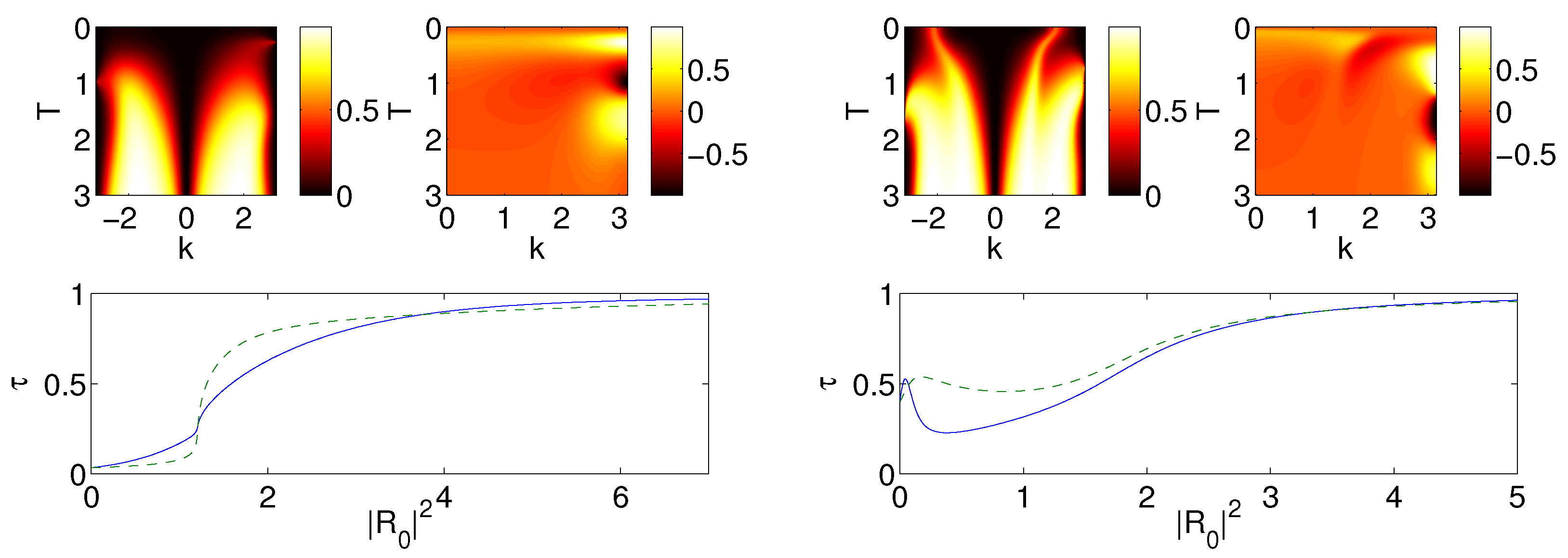
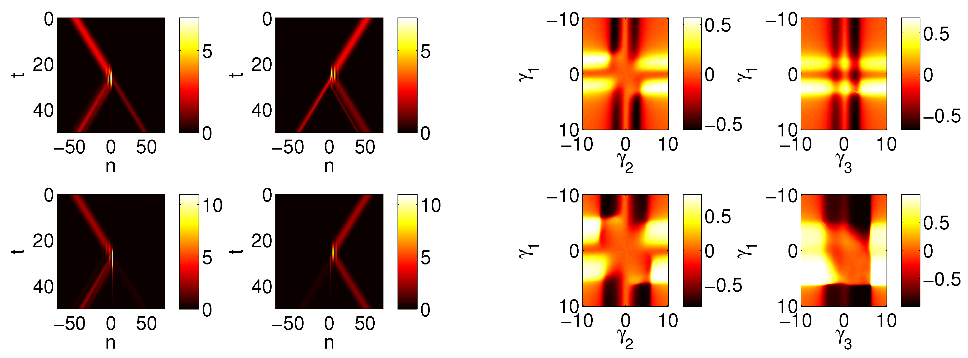
Figure 1 shows plots of the transmission coefficient
τ and the rectification factor
f as a function of the amplitude
T and the wavenumber
k of the extended plane wave solutions. We find that whether more is transmitted for waves incoming from the right or left is variable as a function of
k and
T. Notice that values for
γ’s are chosen in
Figure 1 to be such that
in the
case and
in the
case. In other words, with increasing
γ’s from left to right we observe that transmission properties vary with the choice of the parameters
. We find that in accordance with our above analysis the
case is symmetric. Although we do not show an
analogue of
Figure 1, such plots look similar to
Figure 1 but there is exact symmetry and
for all
. It is interesting to point out here that the rectification factor appears to acquire its largest (absolute) values for
k close to
π i.e., at the edge of the Brillouin zone. Furthermore, both in the
and in the
case, the dependence of
f near this value appears to be a non-sign-definite function of
T (
i.e., different ranges of
T values appear to favor propagation in one or the other direction).
Figure 1.
Each panel contains a contour plot of the transmission coefficient
(
top left) and a contour plot of the rectification factor
of Equation (
9) (
top right), plotted as a function of
k and
T. The panels also show a typical example of the dependence of
τ for
(solid lines) and
(dashed lines), so as to illustrate the asymmetry between the propagation for left and right incident waves (
bottom panel). In the latter the dependence of
τ is given as a function of
. The left panel corresponds to
and
,
and the lattice size is
in this case. The right panel is the
case with
,
and
; here the lattice size is
.
3.2. Stability
In order to analyze the spectral stability of stationary states of the form discussed in the previous subsection we write
for
,
ε small, and with
being a stationary solution from the previous section. The resulting linear stability equations then read
for
where
G is a sparse matrix with ones on both the super- and sub-diagonals. Given a stationary plane wave solution
and values of
which encode the nonlinearity for
, one then calculates the eigenvalues
ν in Equation (
11). If
ν has a negative imaginary part this indicates that the perturbed solution
is unstable, as is easily seen by Equation (
10). In practice, one diagonalizes a finite truncation of the matrix in Equation (
11), ensuring that the relevant eigenvalues are not affected by the truncation error. In other words,
and
G are all
matrices and in the matrix Equation (
11) it is now convenient to think of
and
as length
L column vectors. Furthermore, the Hamiltonian symmetry of the solution ensures that the relevant instability eigenvalues come either in pairs (if
ν is imaginary) or in quartets (if
ν is genuinely complex).
In
Figure 2 and
Figure 3 we show a plot of
as a function of
T and
γ. We find that an increase in the magnitude of a
parameter (with other nearby
γ’s held fixed) leads to
of larger magnitude indicating greater instability.
Figure 2,
Figure 4,
Figure 5 and
Figure 6 show eigenvector and eigenvalue plots alongside snapshots of
to show the behaviour of typical propagation in the
t variable of the unstable plane waves. The boundary conditions are calculated according to Equation (
4) at
and evolved by multiplying by
for
so as to conform with Equation (
10). The unstable plane wave solution, when propagated in the evolution variable, exhibits a few effects: if
then amplitude leaks over to the right-hand side (to the left if
), and due to the localized instability a peak appears in the center of the lattice. Of course, given the conservation laws of the system, the power
and the Hamiltonian
are preserved over
t. The figures also show a transition in the eigenvalue plots for unstable solutions. A weak instability (corresponding to dim but nonzero regions of the
plots of
Figure 2 and
Figure 3) results in eigenvalue plots in the complex plane where a quartet appears off the real axis; see
Figure 2 and
Figure 5. As the instability is enhanced for larger values of
γ (comparably brighter regions of the
plots), the two pairs constituting the quartet merge on the imaginary axis and subsequently split with one pair headed towards zero; see
Figure 4 and
Figure 5. For the highest magnitude of instability (brightest regions on the plots of
) the eigenvalues indicating the instability are in the form of a pair on the imaginary axis; see
Figure 4 and
Figure 6. In the examples shown, the instability generically appears to transport power to the right part of the lattice, deforming (decreasing the power of) the corresponding
portion of the plane wave. On the other hand, critically (per the localized eigenvector of the instability), a localized mode appears to form at the central nonlinear nodes within the domain.
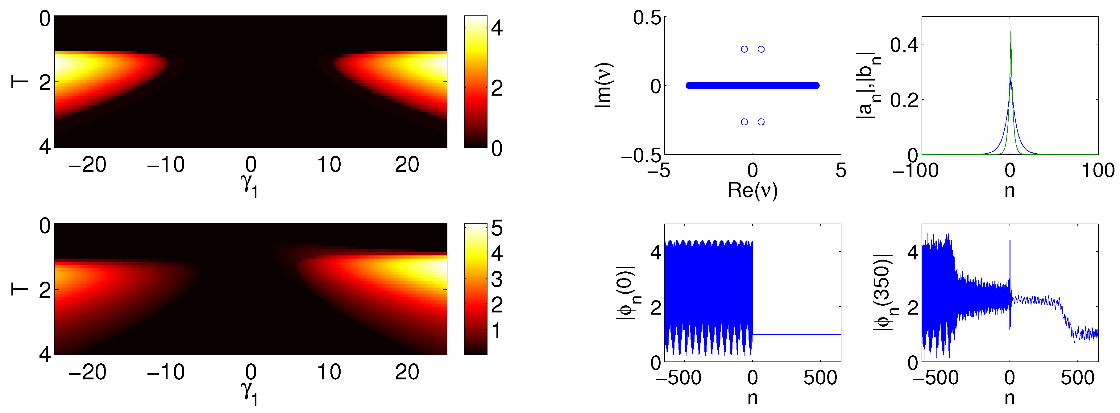
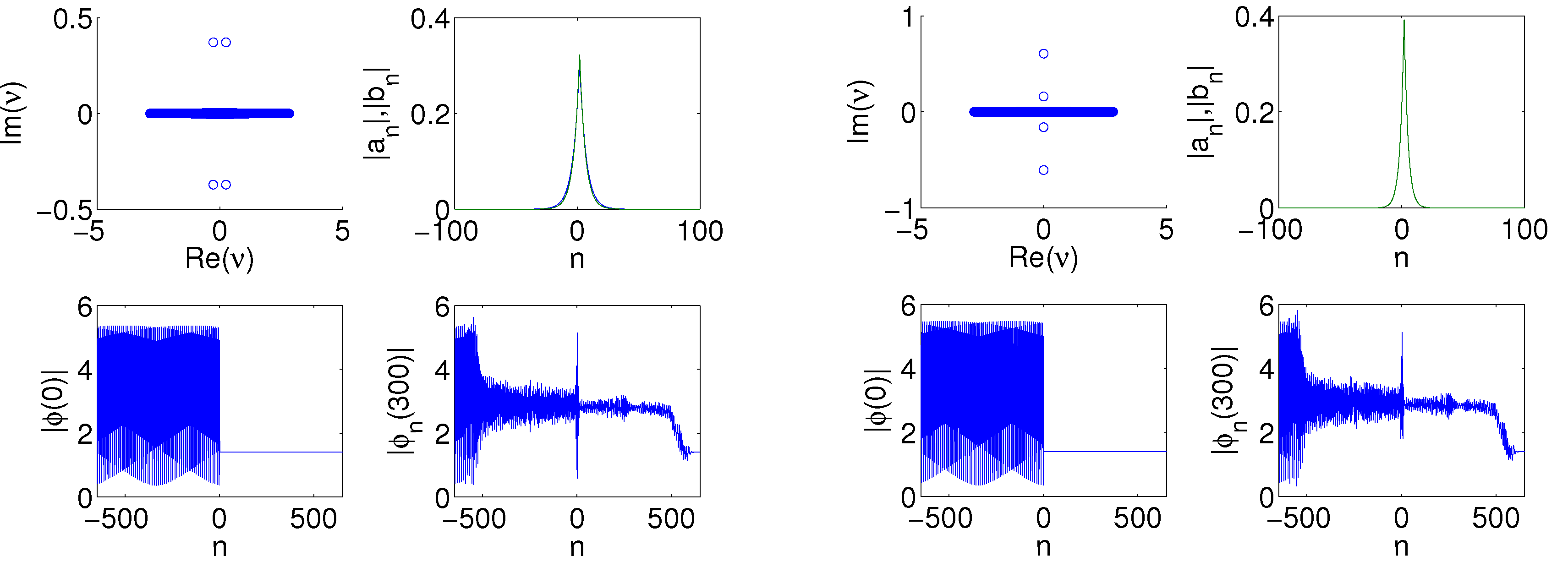
Figure 2.
The left panel depicts the value of
, for
, plotted as a function of
and
T; the top graph shows
and in the bottom graph
. The lattice length in the two left panel plots is
. These two plots show that the magnitude of the minimum imaginary part of the calculated eigenvalue,
i.e., the strength of the instability, increases as the magnitude of
increases. On the other hand for a fixed
value an extended solution of the form shown in Equation (
4) is tending toward stabilization for large
T. In the right panel we show four plots that correspond to a dim but nonzero region on the plot of
in the left panel. That is, the right-hand four plots correspond to
,
and
. The four plots show the eigenvalues in the complex plane (top left), eigenvector magnitude (top right with
blue and
green), initial profile of the plane wave at
(bottom left) and a later profile at
of the plane wave (bottom right). For this instability the eigenvalues are in the form of a quartet.
![Photonics 01 00390 g002]()
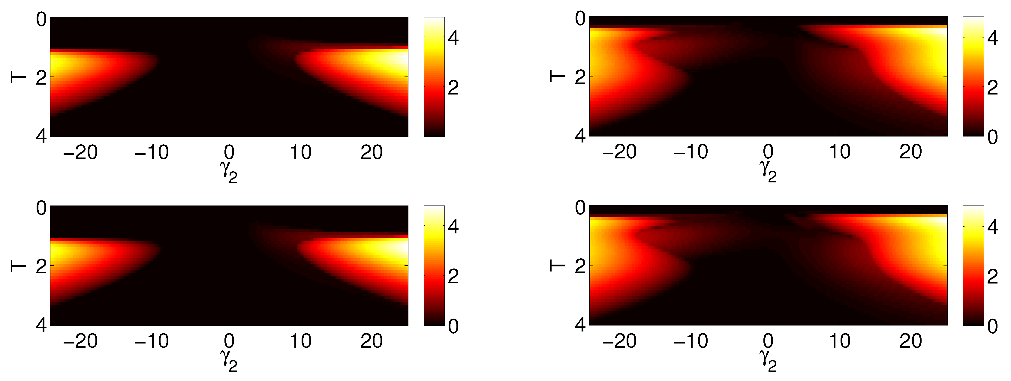
Figure 3.
The plots are similar to the left panel in
Figure 2. Here the left panel corresponds to
,
and we plot
as a function of
and
T while the value of
is fixed:
in the top graph and
in the bottom graph. Here the right panel corresponds to
,
and we plot
as a function of
and
T while the values of
and
are fixed:
,
in the top graph and
,
in the bottom graph.
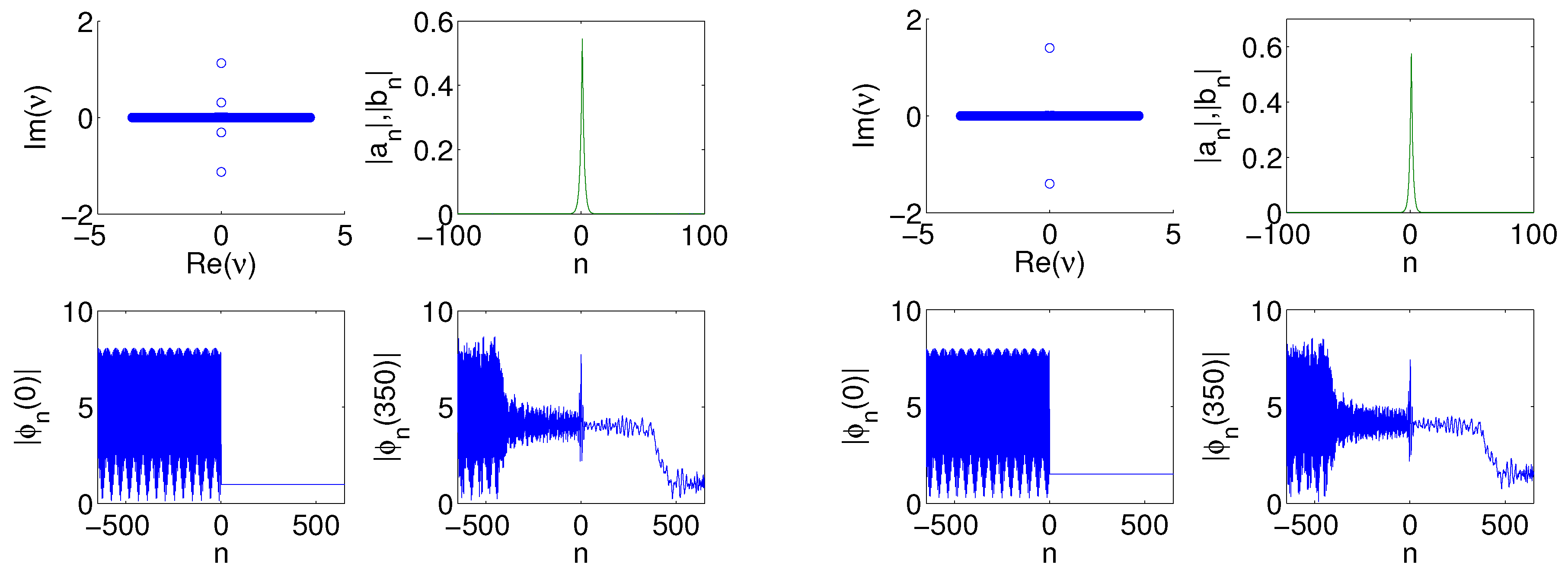
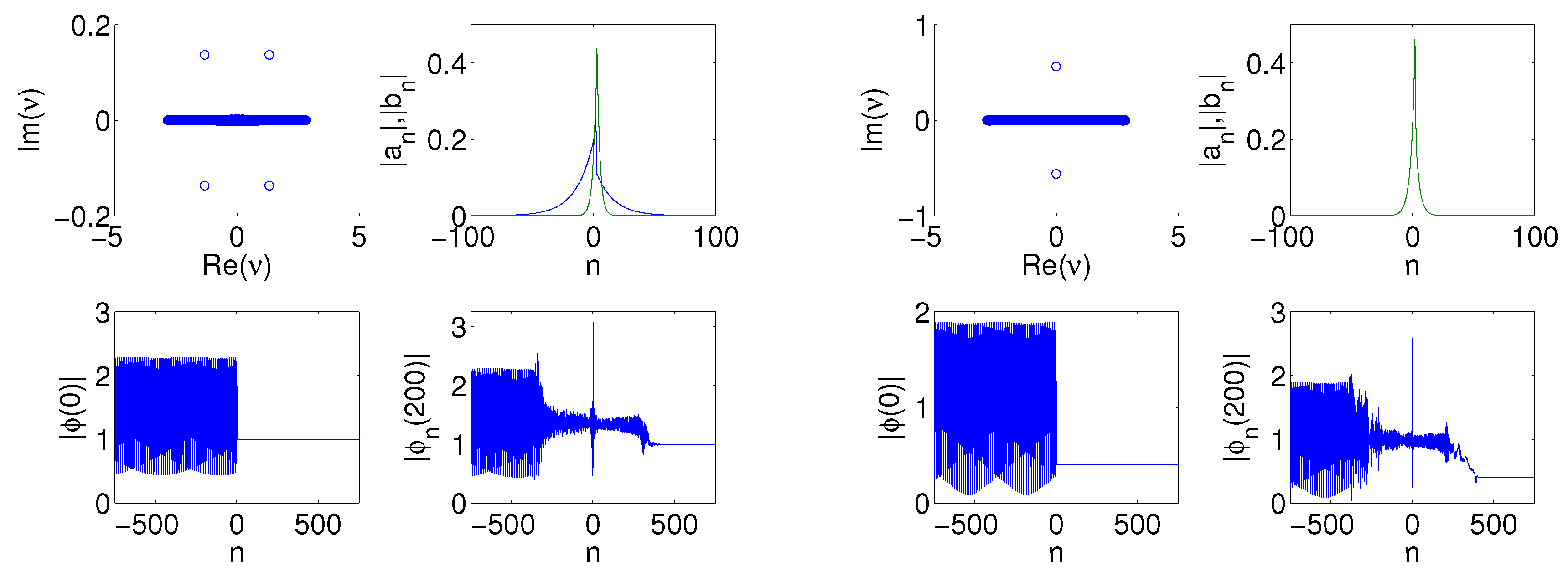
Figure 4.
Here we focus on parameter values that correspond to a bright region in the left panel of
Figure 2. We show four plots similar to the right panel of
Figure 2. Here we have
,
and
. The left panel of four plots corresponds to
,
, and the right panel corresponds to
,
. Comparing the three sets of four plots in the present figure and in
Figure 2 shows the transition in the eigenvalue plots as we move towards brighter regions of the
diagram.
Figure 5.
Here we focus on parameter values that correspond to the left panel of
Figure 3. Again we show four plots similar to the right panel of
Figure 2. Here we have
,
and
. The left panel of four plots corresponds to
,
, and the right panel corresponds to
,
. Comparing these two sets of four plots shows the transition in the eigenvalue plots as we move towards brighter regions of the appropriate
diagram in
Figure 3.
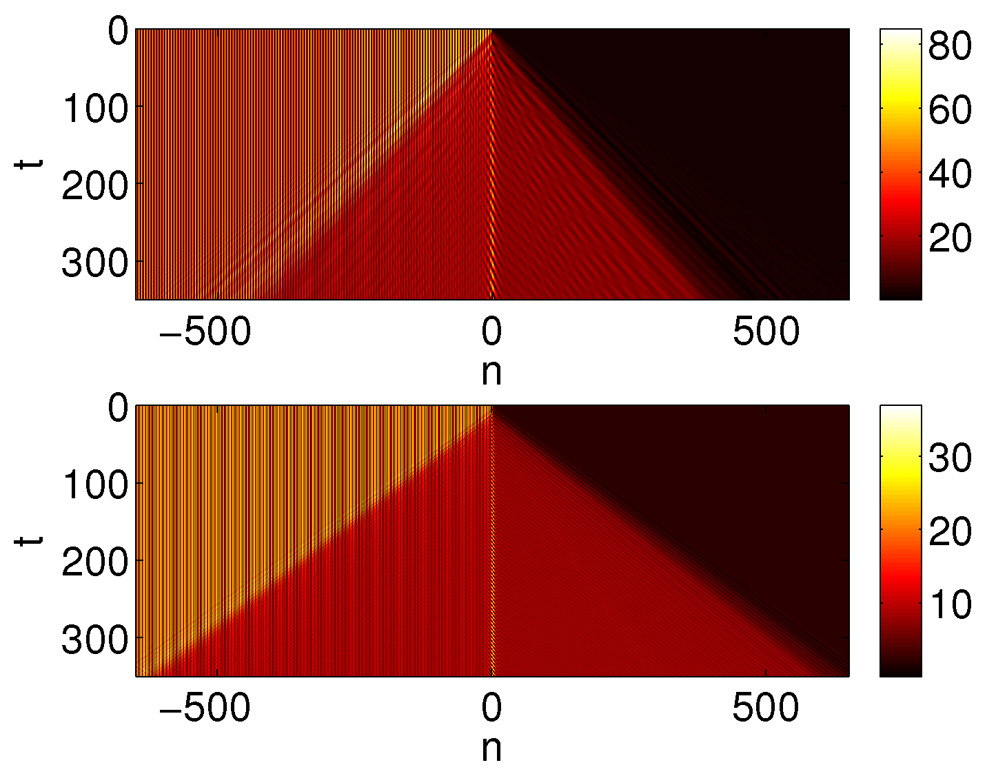
In comparing our results with those of [
19], we find that the asymmetry associated with the saturable nonlinearity (presented here) is less pronounced than that of a system with a cubic nonlinearity and a linear potential term (presented in [
19]). In the
t propagation of extended solutions we can also compare the top plot in
Figure 3 of [
19] with our
Figure 7 in which we show plots over space and the propagation parameter. The two systems both experience a concentration of amplitude at the center of the lattice as
t moves forward. In the case of the cubic nonlinearity in [
19] there are three concentrations of amplitude (two of which are moving). Here we see predominantly a concentration of amplitude at the center, while the large amplitude sites nearby decrease in amplitude in comparison to their respective values at the initialized state at t = 0. Also, in contrast to [
19] where the amplitude concentrations more dramatically rise above the background, here the central concentration of amplitude is more similar to the maximal amplitude of the initialized state.
Figure 6.
Here we focus on parameter values that correspond to the right panel of
Figure 3. Again we show four plots similar to the right panel of
Figure 2. Here we have
,
and
. The left panel of four plots corresponds to
,
, and the right panel corresponds to
,
. Comparing these two sets of four plots shows the transition in the eigenvalue plots as we move towards brighter regions of the appropriate
diagram in
Figure 3.
Figure 7.
The plots show
as a function of
n and
t. The top plot corresponds to parameters the same as in the right four plots in
Figure 4. The bottom plot corresponds to parameters the same as in the left four plots in
Figure 5.
Figure 7.
The plots show
as a function of
n and
t. The top plot corresponds to parameters the same as in the right four plots in
Figure 4. The bottom plot corresponds to parameters the same as in the left four plots in
Figure 5.


