Combined Modelling of Coastal Barrier Breaching and Induced Flood Propagation Using XBeach

Abstract

Breaching of coastal barriers is a three-dimensional process induced by complex interactions between hydrodynamics, sediment transport and soil avalanching processes. Although numerous coastal barriers are breached every year in many coastal countries, causing dramatic inundations of the nearshore areas, the understanding of the processes and interactions associated with both breaching and subsequent flood propagation is still poor. This might explain why their combined modelling and prediction has not yet been sufficiently addressed. Consequently, barrier breaching and subsequent inundation are still often modelled separately, thus ignoring the strong interaction between breaching and flooding. However, the combined modelling of such strongly coupled processes is crucial. Since the open-source model system “XBeach” consists, among others, of a nonlinear shallow water solver coupled with a morphodynamic model, also including a soil avalanching module, it has the potential to simulate both breaching and subsequent flood propagation together. Indeed, the mutual interactions between hydrodynamics and morphodynamics (including soil avalanching) are properly accounted for. This paper, therefore, aims to examine the applicability of XBeach for modelling coastal barrier breaching and inundation modelling in combination, instead of the current approaches, which address the modelling of each of these two processes separately. The performance of XBeach, in terms of inundation modelling, is assessed through comparisons of the results from this model system (i) with the results from common 1D and 2D flood propagation models and (ii) with observations for barrier breaching and subsequent inundation from a real case study. Besides providing an improved understanding of the breaching process, the results of this study demonstrate a new promising application of XBeach and its potential for calculating time-varying inland discharges, as well as for combined modelling of both dune breaching and subsequent flood propagation in coastal zones.

1. Introduction

Coastal floods induced by extreme storm surges are among the most destructive natural disasters. They may become even more destructive (Smith, 2013 [1]; Lilai et al. 2016 [2]), especially when these floods result from coastal barrier breaching, where significant inland flow with very high velocities can extend widely in the hinterland in a relatively short time (Kraus and Wamsley, 2003 [3]; Roger et al. 2010 [4]; Bisschop et al. 2010 [5]; Wu et al. 2011 [6]). Catastrophic coastal floods are generally associated with loss of lives and injuries, as well as significant direct and indirect economic losses (e.g., Sills et al. 2008 [7]). In addition to these losses, coastal floods may have severe environmental and ecological consequences, e.g., groundwater contamination due to saltwater intrusion into aquifers (e.g., Yang et al. 2013 [8]; 2015 [9]).

The prediction of a storm-induced flood through a breach-induced inlet represents a real challenge because storm-induced breaches represent a multi-scale problem governed by complex interactions between a large variety of relatively uncertain hydrodynamic and sediment-related processes at different time and length scales (Wu et al. 2011 [6]; Christensen et al. 2013 [10]; He et al. 2015 [11]). These processes and interactions are, for instance, (i) combined water level rise and increased wave exposure during a storm surge, (ii) coastal barrier erosion and breach development, and (iii) subsequent flow into the hinterland and inundation during/after completion of the breach growth. The entirety of all these processes constitutes coastal flooding as a physical system with its own characteristic dynamics. Because the outcomes of this system may lead to catastrophic consequences (e.g., Hinkel et al. 2014 [12]), it is important to analyse these system dynamics as well as the expected consequences and the human intervention of such a system. For this purpose, the knowledge of the distribution of the maximum water levels in the flooded area(s) as well as the description of the path and the temporal propagation of the inundation by considering the size and shape of the flood prone area, its topography and any obstacles that can block or hinder the development of the flood, are crucial. In fact, they represent important and useful information to the decision makers, if implemented in rescue and emergency plans for the flood prone area (Cheung et al. 2003 [13]). Moreover, they can be used to estimate the economic and the environmental consequences of a flood.

The main issue when modelling coastal inundation is the assessment of the volume flux of water that passes the sea defences (i.e., the inland flow hydrograph Q(t)) during an overtopping/overflow event and/or through a breach induced inlet. In earlier studies of coastal flooding (e.g., Bates et al. 2005 [14], Chini et al. 2012 [15] and Smith et al. 2012 [16]), this information has often been missing. Only rough estimates could be proposed based on volume reconstruction using, for instance, aerial photographs to estimate the flood extent and then working out the water volume and hence the mean flow rate during the coastal inundation event. As a result, the mean flow rate is used as the input for a common flood model to numerically reproduce the flood event. For the same purpose, other studies (e.g., McCabe et al. 2013 [17], Chini and Stansby, 2012 [18], Gallien et al. 2014 [19], Tsoukala et al. 2016 [20]) attempted to estimate temporally variable overflow rates along representative discrete transects using the empirical equations and/or neural network tool recommended by static models (e.g., EurOtop of Pullen et al. 2007 [21]). However, the inundation extent, calculated based on such static models, is often substantially overestimated when compared to real flood extent observations (Gallien et al. 2014 [19]; Vousdoukas et al. 2016 [22]). Moreover, such empirical models cannot be used to calculate the inland discharge through a breach induced inlet because of the dynamic nature of the breaching process, which cannot be analysed based on static and empirically-based overtopping/overflow models (e.g., EurOtop) by simply comparing water levels and land elevations. Recently, XBeach, a coastal hydro-morphodynamic open-source model developed with funding and support by the US Army Corps of Engineers, the consortium of UNESCO-IHE, Deltares, Delft University of Technology and the University of Miami (Roelvink et al. 2009 [23]), has been used in few studies (e.g., Giardino et al. 2011 [24], Barnard et al. 2014 [25], Gallien and Guza, 2015 [26] and Gallien, 2016 [27]) to numerically estimate temporally variable overtopping volumes (in the form of intermittent overtopping rates) along representative discrete transects. The latter are also applied as input conditions for a common inundation model. The comparison between the overtopping rates calculated by static models (e.g., EurOtop) and dynamic models (e.g., XBeach) showed that the outcomes of the latter are more accurate (Gallien, 2016 [27]). In fact, XBeach can predict overtopping rates with a relatively high coefficient of regression (R² = 0.87) (Palmsten and Splinter, 2016 [28]). However, the application of XBeach in coastal inundation studies is still limited to the estimation of wave overtopping rates.

To date, the modelling of coastal flood induced by overtopping is based on two subsequent and uncoupled modelling approaches:

(i)

empirical model (e.g., EurOtop) or numerical model (e.g., XBeach) to predict overtopping rates along representative discrete transects for overland flow model input, and

(ii)

Computational Fluid Dynamics (CFD) solver used as inundation models to simulate the overland and surface runoff using the results from the overtopping models as input conditions (Wadey et al. 2012 [29]; Gallien, 2016 [27]; Worni et al. 2014 [30]). Such CFD models (e.g., River-2D, ISIS-2D, BASEMENT-2D, MIKE FLOOD, BreZo, DIVAST, TELEMAC-2D, TUFLOW or SOBEK) are generally based on the solution of the nonlinear shallow water equations (NLSWEs).

Similarly, the current modelling of a breach-induced flood is based on two subsequent and uncoupled modelling approaches:

(i)

breaching model (e.g., XBeach) to calculate the flow rates through a breach-induced inlet and

(ii)

CFD model as described above to simulate the inundation resulting from the breach.

Indeed, such modelling approaches are more common in fluvial environments than in coastal environments, especially when analysing breaching-induced floods at conditions when a landslide dam retards the flow in a river stream (e.g., Elsayed, 2013 [31]; Radice and Elsayed, 2014 [32]; Fan et al. 2012 [33]; Popescu et al. 2010 [34]). The weaknesses of such uncoupled modelling approaches arise from the need to “manually” transfer the outcomes of the overtopping/breaching model to the inundation model. Moreover, by dividing the whole system into two subsystems, such separate modelling approaches partially omit the continuity of the processes and their interactions in both subsystems. Among these subsystems, the mass (flow) can be transferred in the form of inland hydrograph, but the flow velocity and thus the momentum cannot, which means that the momentum conservation principle is usually omitted through the flow transition between these subsystems. Though the momentum is mostly of importance close to the breach, the omission of the momentum transfer between the decoupled breaching and inundation models would also affect the far field, even to a lesser extent. In fact, the far field will be affected much less than the near field as shown, for instance, in Figures 8 and 9, showing that the water levels obtained from both coupled and decoupled approaches tend to converge in the far field.

In order to overcome the weaknesses of such separate modelling approaches, combined modelling of overtopping/breaching of coastal barriers under extreme storm surges and subsequent coastal flooding is crucial. As a result, a single model system can carry out the computations over a single calculation mesh containing both the bathymetry of the nearshore area and the topography of the shore/hinterland. Indeed, many studies (e.g., Christensen et al. 2013 [10]; Tadesse et al. 2014 [35]; He et al. 2015 [11]; Bertin et al. 2014 [36]; Roland et al. 2012 [37]; Vousdoukas et al. 2016 [38]) attempted to simulate storm surges and the induced coastal flooding in a single model. However, in these studies either the morphodynamics and thus the storm-induced breaches are omitted (e.g., Bertin et al. 2014 [36]; Roland et al. 2012 [37]; Vousdoukas et al. 2016 [38]) or a proper breaching/morphological module is lacking (e.g., Christensen et al. 2013 [10]; Tadesse et al. 2014 [35]; He et al. 2015 [11]). However, all these studies were based on solving the NLSWEs over a single calculation mesh that contains the bathymetry of the nearshore area and the topography of the shore/hinterland.

The model system XBeach also includes a solver for the NLSWEs (CFD module) as well as a morphodynamic solver together with a soil avalanching module, which revolves around a user-defined critical slope. Therefore, its application can be extended to simulate coastal inundation, together with overtopping/breaching in a single model system, using a unique calculation mesh for both CFD and morphodynamic modules. While the morphodynamic solver is applied to simulate sediment transport and morphological changes, including breach development, the CFD solver is used for the combined modelling of overtopping and overflow processes, the flow through the developing breach and the subsequent coastal inundation processes. In addition to overcoming the aforementioned weaknesses of the separate modelling approaches, such combined modelling provides the advantages of (i) simulating the mutual interaction between hydrodynamics and morphodynamics, including soil avalanching, and (ii) considering the longshore variability of the hydraulic load and/or the coastal barrier topography. XBeach, on the other hand, is a freely available open-source code, which means that users can make changes to the programme through changes to the code itself, to suit the needs of individual users and projects. Moreover, the model is being continuously improved by applications in diverse coastal environments worldwide in order to include all the nearshore processes, which are not included yet in the model (e.g., Elsayed and Oumeraci, 2016 [39] and Bendoni, 2015 [40]). Furthermore, XBeach has been successfully applied to simulate barrier breaching in coastal environments (e.g., Roelvink et al. 2009 [23]; De Vet, 2014 [41]) and also to flood propagation in fluvial environments (Hartanto et al. 2011 [42]; Beevers et al. 2016 [43]). However, to the authors’ knowledge, XBeach has not yet been applied as an inundation model and a breaching model in combination. Moreover, no study has yet attempted to even calculate the inland discharge through a breach induced inlet using XBeach. For the latter reasons, the current applications of XBeach in coastal inundation studies are, as yet, limited (i) to the estimation of overtopping rates along representative discrete transects for overland flow model input or (ii) to the reproduction of previous overwash/breaching events without exploiting the overwash/breaching outcomes in coastal inundation studies.

This paper, therefore, aims

(i)

to extend the scope of using XBeach by examining its applicability for modelling coastal barrier breaching and inundation modelling in combination, instead of the current approach, which addresses the modelling of each of these two processes separately,

(ii)

at a comparative analysis of the results from the latter approach (decoupled approach) with the results of the proposed combined modelling approach using XBeach,

(iii)

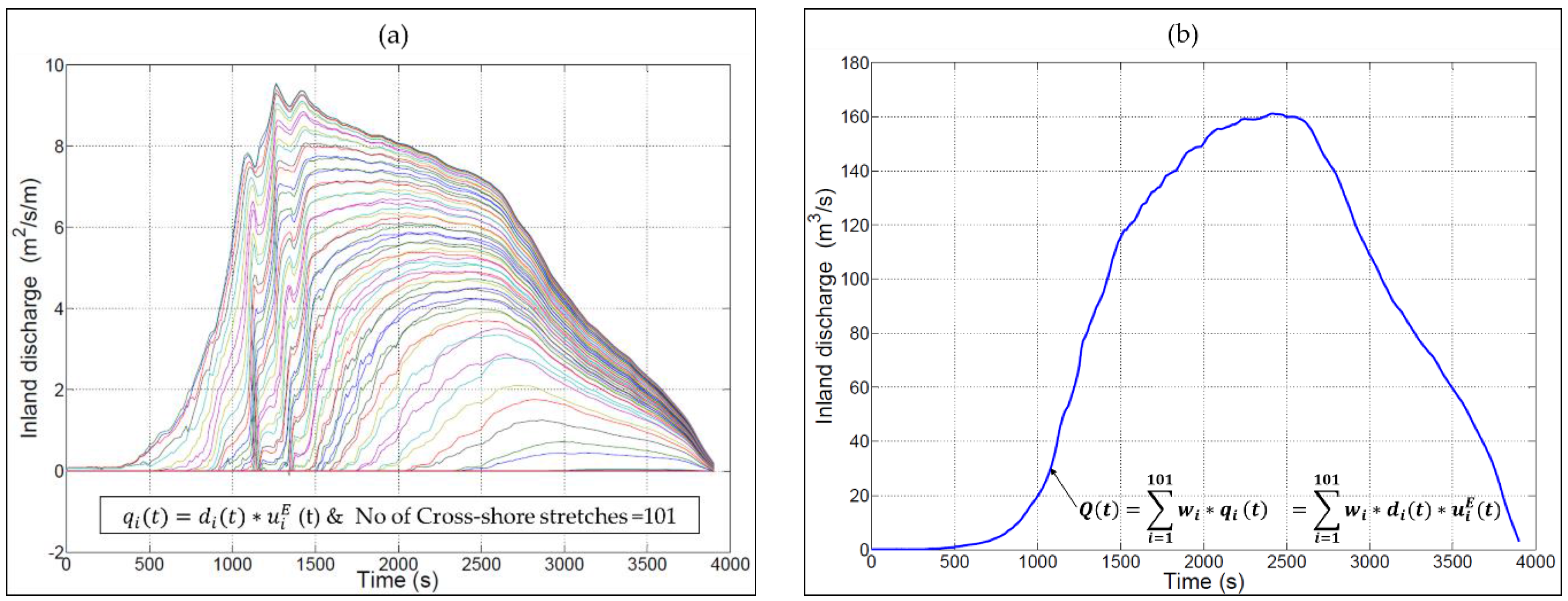
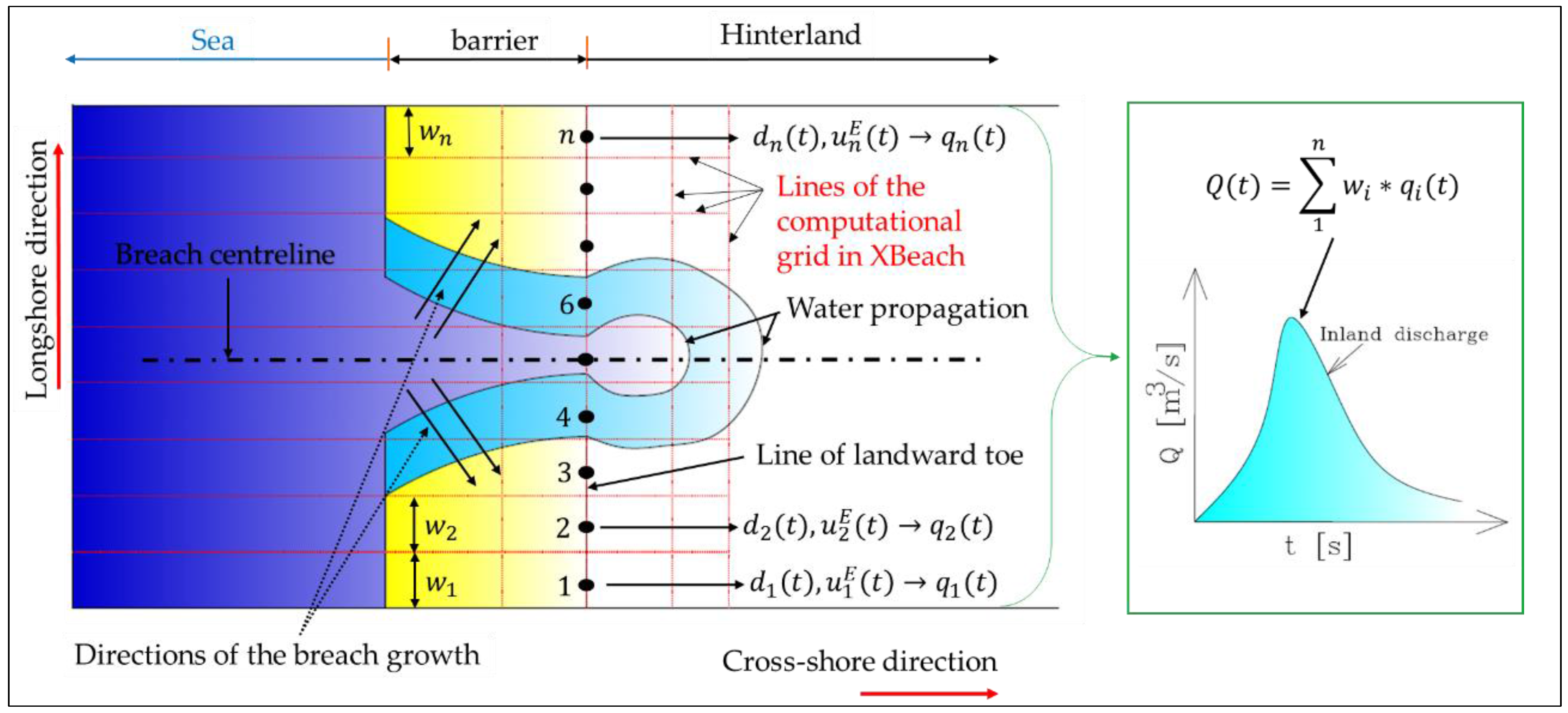
to introduce a computing technique for calculating the flow through breaches reproduced by XBeach (inland hydrograph), and

(iv)

to improve the understanding of the processes and interactions associated with both breaching and subsequent flood propagation.

The examination of the XBeach performance as an inundation model is carried out through comparisons:

(i)

with the results from common 1D and 2D CFD models for flood propagation (e.g., Hydrologic Engineering Center’s River Analysis System (HEC-RAS)(1D) and River-2D)), using the calculated inland hydrograph through a breach-induced inlet(s) as the upstream inflow condition for these models and

(ii)

with observations for breaching and subsequent inundation from a real case study.

The paper is structured as follows: Section 2 provides a brief overview of the numerical models applied in this study, including the hydro-morphodynamic model XBeach, and the 1D model HEC-RAS and River-2D model (both for inundation), besides highlighting the main differences between XBeach and both inundation models. Section 3 describes synthetic and real cases that are applied to assess the performance of XBeach. Section 4 describes the study results, Section 5 discusses the results and Section 6 presents the study conclusions.

2. Methods

The circulation of water in oceans, seas and rivers is a three-dimensional (3D) process, which is usually analysed using the 3D continuity equation and the 3D Navier–Stokes equations that are obtained, respectively, from mass and momentum conservation principles (Vreugdenhil, 2013 [44]; Weiyan, 1992 [45]). However, circulation in flumes, flooded straight roads, estuaries, rivers and cross-shore coastal profiles can be simplified and simulated using a one-dimensional (1D) version of the continuity and momentum equations which are known as Saint-Venant equations (Saint-Venant, 1871 [46]). For studies related to nearshore water circulation, and also often for modelling coastal flooding and the induced inland inundation, the vertical velocity component in the full 3D Navier–Stokes equations can be neglected. As a result, the so-called (2D) shallow-water equations is obtained, which is the case of the CFD module in XBeach and the common inundation models (e.g., River-2D of Steffler and Blackburn, 2002 [47]).

In this study, three numerical codes are used: HEC-RAS, River-2D and XBeach. XBeach is applied over a single calculation grid to simulate nearshore processes, induced overtopping, overwash and/or breaching as well as flood propagation in the hinterland. The application of HEC-RAS and River-2D is limited only to examine the XBeach performance for flood propagation in the hinterland, where the inland discharge computed from XBeach at the landward toe of the coastal barrier is used as an upstream input to the inundation models HEC-RAS or River-2D. Therefore, both inundation models simulate the hydrodynamics over a grid containing only the topography of the shore/hinterland. Examining the XBeach performance as an inundation model is required because the validity of XBeach outside its original application domain (nearshore hydrodynamics and morphodynamics) needs first to be comprehensively tested. As a result, the applicability of XBeach in inundation modelling may open the door to a greater number of users beyond the current applications. Moreover, such an examination also enables assessing the current approaches for modelling coastal floods (i.e., the one-way coupling between the overtopping/breaching model and another inundation model) as compared to the proposed approach using XBeach to simulate both overtopping/breaching and subsequent inundation in combination. The following subsections provide a brief overview of the three aforementioned codes.

2.1. HEC-RAS

HEC-RAS is a 1D St. Venant model developed by the US Army Corps of Engineers to manage river flow. The HEC-RAS software has found wide acceptance among hydraulic engineers and researchers due to its robust channel flow analysis capabilities and its ability to determine floodplain areas. Furthermore, HEC-RAS uses steady and unsteady state modelling routines based on solving the full 1D St. Venant equations (Equations (1) and (2)) for unsteady open channel flow:

$$\frac{\partial Q}{\partial x}+\frac{\partial A}{\partial t}=0$$

(1)

$$\underset{\begin{array}{c}\mathrm{Inertial}\\ \mathrm{force} \mathrm{term}\end{array}}{\underbrace{\underset{\begin{array}{c}\mathrm{Local} \\ \mathrm{acceleration} \end{array}}{\underbrace{\frac{\partial u}{\partial t}}}+\underset{\begin{array}{c}\mathrm{Convective} \\ \mathrm{acceleration} \end{array}}{\underbrace{u . \frac{\partial u}{\partial x}}}}}+\underset{\begin{array}{c}\mathrm{Pressure} \\ \mathrm{force} \mathrm{term}\end{array}}{\underbrace{g . \frac{\partial d}{\partial x}}}+\underset{\begin{array}{c}\mathrm{Gravity} \\ \mathrm{force} \mathrm{term}\end{array}}{\underbrace{g .S_0}}=\underset{\begin{array}{c}\mathrm{Friction} \\ \mathrm{force} \mathrm{term}\end{array}}{\underbrace{g .S_f}}$$

(2)

Q (x,t) is the discharge [m³/s], x is the longitudinal distance along the flow direction [m], A is the flow cross-sectional area [m²], t is time [s], u is the depth-averaged flow velocity [m/s], g is the gravitational acceleration 9.81 [m/s²], d is the water depth [m], $S_o$ is the bottom slope [-] and $S_f$ is the bed friction slope [-] (for the fully turbulent flow, the bed friction slope can be described by $S_f=\frac{u^2}{C_{ch}^2\ast R_H}$, where $C_{ch}$ is the Chezy coefficient [$m^{\frac{1}{2}}/s$], $R_H$ is the hydraulic radius [m]). The balance of the discharge (mass) in and out a control volume is determined in the model through the continuity equation (Equation (1)) while the balance of forces (momentum) within the same control volume is determined by the momentum equation (Equation (2)) in the form of accelerations balance, including inertial (local + convective), pressure, gravity and friction accelerations. These equations are discretized using the finite difference method and solved using a four point implicit (box) method (Szymkiewicz, 1996 [48]). In addition to solving the St. Venant equations, HEC-RAS can calculate the sediment transport potential using simple formulae, e.g., the formula of Meyer-Peter and Muller, 1948 [49] (Pender et al. 2015 [50]; Brunner, 2016 [51]).

2.2. River-2D

The River-2D model (Steffler and Blackburn, 2002 [47]) is a finite element solver for the two-dimensional (2D) depth-averaged NLSWEs (Equations (3)–(5)). It was developed by the University of Alberta, Edmonton, Alberta, Canada. The River-2D suite actually consists of three main programmes: R2D_Bed, R2D_Mesh and River-2D. These programmes are typically used in succession, in which the normal modelling process would involve creating a preliminary bed topography file from raw field data, then editing and refining it using R2D_Bed. The resulting bed topography file is used in R2D_Mesh to develop a computational discretization based on the Triangulated Irregular Network (TIN) methodology as input to River-2D, which is then used to solve for the water depths and velocities throughout the discretization and to visualise and interpret the results.

$$\frac{\partial z_s}{\partial t}+\frac{\partial \left(d·u\right)}{\partial x}+\frac{\partial \left(d·v\right)}{\partial y}=0$$

(3)

$$\frac{\partial u}{\partial t}+u · \frac{\partial u}{\partial x}+v · \frac{\partial u}{\partial y}-{\nu }_h\left(\frac{{\partial }^{2}u}{\partial x^2}+\frac{{\partial }^{2}u}{\partial y^2}\right)=\frac{{\tau }_{sx}}{\rho d}-\frac{{\tau }_{bx}}{\rho d}-g ·\frac{\partial z_s}{\partial x}$$

(4)

$$\underset{\begin{array}{c}\mathrm{Inertial}\\ \mathrm{force} \mathrm{term}\end{array}}{\underbrace{\underset{\begin{array}{c}\mathrm{Local} \\ \mathrm{acceleration} \end{array}}{\underbrace{\frac{\partial \text{v}}{\partial \text{t}}}}+\underset{\begin{array}{c}\mathrm{Convective} \\ \mathrm{acceleration} \end{array}}{\underbrace{u . \frac{\partial v}{\partial x}+v . \frac{\partial v}{\partial y}}}}}-\underset{\begin{array}{c}\mathrm{Transverse} \mathrm{Shear}\\ \mathrm{stresses} \mathrm{term}\end{array}}{\underbrace{{\nu }_h\left(\frac{{\partial }^{2}v}{\partial x^2}+\frac{{\partial }^{2}v}{\partial y^2}\right)}}=\underset{\begin{array}{c}\mathrm{surface} \mathrm{shear}\\ \mathrm{stresses} \mathrm{term}\end{array}}{\underbrace{\frac{{\tau }_{sy}}{\rho d}}}-\underset{\begin{array}{c}\mathrm{Friction} \\ \mathrm{forces} \mathrm{term}\end{array}}{\underbrace{\frac{{\tau }_{by}}{\rho d}}}-\underset{\begin{array}{c}\mathrm{pressure} \\ \mathrm{forces} \mathrm{term}\end{array}}{\underbrace{g .\frac{\partial z_s}{\partial y}}}$$

(5)

$z_s$ is the water surface level [m], $z_b$ is the bed level [m] so that the water depth $d = z_s – z_b$, $u$ and $v$ are the depth-averaged flow velocities per meter width [m/s] in x- and y- directions, ${\nu }_h$ is the horizontal eddy viscosity coefficient [$m^2/s$] that is computed in River-2D using a Boussinesq-type formulation (Steffler and Blackburn, 2002 [47]) and $\rho$ is the water density [$kg/m^3$]. ${\tau }_{sx}\mathrm{and}{\tau }_{sy}$ are the components of the surface shear stresses [$N/m^2$] while ${\tau }_{bx}\mathrm{and}{\tau }_{by}$ are the components of the bed shear stresses [$N/m^2$], where ${\tau }_{bx}=\rho g·d·S_{fx}$ and ${\tau }_{by}=\rho g·d·S_{fy}$. The friction slope terms $s_{fx}$ and $s_{fy}$ depend on the bed shear stresses that are assumed to be related to the magnitude and direction of the depth averaged velocities and a dimensionless bed friction coefficient $c_f$ (Steffler and Blackburn, 2002 [47]) as follows.

$${\tau }_{bx}= \rho ·g ·d·s_{fx}=c_f·\rho · u· \sqrt{u^2+v^2}\text{ with }{\tau }_{by}=\rho ·g ·d·s_{fy}=c_f·\rho · v· \sqrt{u^2+v^2}$$

(6)

2.3. XBeach

XBeach is a coupled stochastic (phase-averaged) spectral wave model for storm-induced waves and the nonlinear shallow water model for infragravity waves (Roelvink et al. 2009 [23]; Roelvink et al. 2015 [52]). Therefore, XBeach describes short-wave processes in a stochastic manner, solving the phase-averaged wave action equation of Holthuijsen et al. 1989 [53] often based on empirical formulations calibrated to field or laboratory data (Buckley et al. 2014 [54]). However, the infragravity wave motions and mean flows induced mass-flux and the subsequent (return) flow are modelled in a deterministic manner based on mass and momentum conservation laws, solving the NLSWEs using a finite difference scheme, where the short wave induced radiation forces ($F_x$ and $F_y$ [$N/m^2$]) are input as the external source term on the NLSWEs as follows

$$\frac{\partial z_s}{\partial t}+\frac{\partial \left(d · u^L\right)}{\partial x}+\frac{\partial \left(d · v^L\right)}{\partial y}=0$$

(7)

$$\frac{\partial u^L}{\partial t}+u^L. \frac{\partial u^L}{\partial x}+v^L. \frac{\partial u^L}{\partial y}-{\nu }_h\left(\frac{{\partial }^2{u}^L}{\partial x^2}+\frac{{\partial }^2{u}^L}{\partial y^2}\right)=\frac{{\tau }_{sx}-{\tau }_{bx}^E}{\rho d}-g.\frac{\partial z_s}{\partial x}+\frac{F_x}{\rho d}$$

(8)

$$\frac{\partial v^L}{\partial t}+u^L. \frac{\partial v^L}{\partial x}+v^L. \frac{\partial v^L}{\partial y}-{\nu }_h\left(\frac{{\partial }^2{v}^L}{\partial x^2}+\frac{{\partial }^2{v}^L}{\partial y^2}\right)=\frac{{\tau }_{sy}-{\tau }_{by}^E}{\rho d}-g .\frac{\partial z_s}{\partial y}+\frac{F_y}{\rho d}$$

(9)

Comparing Equations (7)–(9) with the NLSWEs for any common inundation model (e.g., Equations (3)–(5) for River-2D), two main differences can be noticed: (i) the representation of the depth-averaged velocities (u and v) and (ii) the short wave induced forces ($F_x$ and $F_y$).

In the NLSWEs of XBeach (Equations (7)–(9)), most of the terms are formulated in terms of the Lagrangian velocities (superscript L), which are defined as the distance a water particle travels in one wave period divided by this period. Only the bed shear stresses (Equation (10)) are formulated in terms of the Eulerian velocities (superscript E) and defined as the short-wave-averaged velocity observed at a fixed point.

$${\tau }_{bx}^E=c_f\rho u^E\sqrt{{\left(1.16u_{rms}\right)}^2+{u^E}^2+{v^E}^2}\text{ with }{\tau }_{by}^E=c_f\rho v^E\sqrt{{\left(1.16u_{rms}\right)}^2+{u^E}^2+{v^E}^2}$$

(10)

$c_f$ is another dimensionless bed friction coefficient equivalent to that in Equation (6) {$c_f=\sqrt{(g/\left(C_{ch}^2 \right)})=\sqrt{\left(\left(g{n}^2\right)/d^{1/12} \right)}$}, n is the Manning coefficient [$s/m^{\frac{1}{3}}$]. The root-mean-squared orbital velocity $u_{rms}$ [m/s] is the short wave orbital velocity that is at bed obtained from the wave group varying wave energy using linear wave theory (Sultan, 1992 [55]) as:

$$u_{rms}=\frac{\pi H_{rms}}{T_{rep}·\sqrt{2}·sinh\left(k\left(d+\delta ·H_{rms}\right)\right)}$$

(11)

$T_{rep}$ is the representative wave period [s], $H_{rms}$ is the root-mean-square wave height [m], $k$ represents the wave number [$m^{-1}$] and $\delta$ states what fraction of the wave height should be added to the water depth in order to account for the wave nonlinearity effect on $u_{rms}$ (Roelvink et al. 2015 [52]).

The NLSWEs of the common inundation models (e.g., River-2D) are formulated in terms of the Eulerian velocities only, i.e., all the velocities in Equations (3)–(5), for instance, are represented by the Eulerian frame of reference in contrast to XBeach, which mixes between the Eulerian and Lagrangian frames. The latter represents one of the main differences between XBeach and any other inundation model. However, this difference vanishes if the shortwave energy is fully dissipated through the transition from the coastal zone to the hinterland. As a result, the formulation of the bed shear stresses in XBeach (Equation (10)) yields to that in Equation (6), which is the formulation of the bed shear stresses in several inundation models (e.g., River-2D or BASEMENT-2D of Vetsch et al. 2016 [56]). XBeach has, therefore, a more generic representation of the bed shear stresses and the depth-averaged velocities, which is known as Generalized Lagrangian Mean (GLM). According to Andrews and McIntyre, 1978 [57] and Walstra et al. 2001 [58], the GLM approach applies to any problem, whose governing equations are given in Eulerian form (e.g., common inundation models), with a more thorough representation of the real processes (e.g., the GLM approach provides a far more direct route to wave dissipation mechanism than does the conventional Eulerian-mean description).

The wave induced forces $F_x$ and $F_y$ represent the second basic difference between XBeach and any other inundation model. The magnitude of these forces depends mainly on the wave energy in deeper water. A significant part of this energy is dissipated due to wave breaking and bed friction effects, as well as due to waves diffraction through the breach-induced inlet (e.g., Ambrosio and Siegle, 2014 [59]). When using XBeach as an inundation model, the flood propagation in the hinterland may be affected by the non-dissipated part of wave energy, i.e., the wave-induced forces might still have considerable values in the hinterland that would affect the propagation kinematics and inundation depths. However, this remaining wave energy is expected to be rapidly dissipated in the hinterland under the bed friction effect. As a result, the terms of the short wave-induced forces in Equations (8) and (9) would vanish quickly in the hinterland and become identical to Equations (4) and (5), which are the momentum equations for the state of the art inundation models. Therefore, XBeach can be applied in both coastal and fluvial environments (Hartanto et al. 2011 [42]; Beevers et al. 2016 [43]). In fluvial environments, velocities are usually described by the Eulerian form of the NLSWEs. As a result, XBeach can simulate the hydrodynamics in both the nearshore area and the hinterland with the capability of simulating the induced morphodynamics, including soil avalanching.

The most interesting feature in the morphodynamic part of XBeach is the inclusion of a soil avalanching algorithm that accounts for the slumping of sandy material from the dune face to the foreshore or from the breach sides to inside the breach (see, e.g., Swartenbroekx et al. 2010 [60], Evangelista et al. 2015 [61], and Wainwright and Baldock, 2015 [62]). Avalanching is introduced in XBeach by introducing a critical bed slope steepness for both dry and wet areas. It is considered that inundated areas are much more prone to slumping. Therefore, two separate critical slopes for dry and wet points are used, which are by default 1.0 and 0.3, respectively. In fact, the default value for the dry slope (1) satisfies the equilibrium profile of Vellinga, (1986 [63]). According to Roelvink et al. (2009 [23]), the latter slope must be seen as an average slope after dune erosion, where some stretches may exhibit vertical slopes and other drier parts may have slumped further. On the other hand, the default value for the underwater critical slope (0.3) is much lower and was estimated based on the maximum underwater slope that was observed at the Het Zwin breach test (Section 3.3 in below). When these critical slopes are exceeded, the material is exchanged between the adjacent cells to the amount needed to bring the slope back to the critical slope.

The previous capabilities of XBeach make it eligible as an inundation model besides being a breaching model. Therefore, XBeach can be used as a breaching and inundation model in combination, rather than using two decoupled models to simulate barrier breaching and subsequent coastal flooding.

3. Test Cases

In the following sections, the performance of XBeach is tested (i) against the results from HEC-RAS and River-2D based on a 1D and 2D synthetic cases, respectively and (ii) against an experimental field case for the breaching of the Het Zwin dam and the subsequent flood propagation (Visser, 1998 [64]).

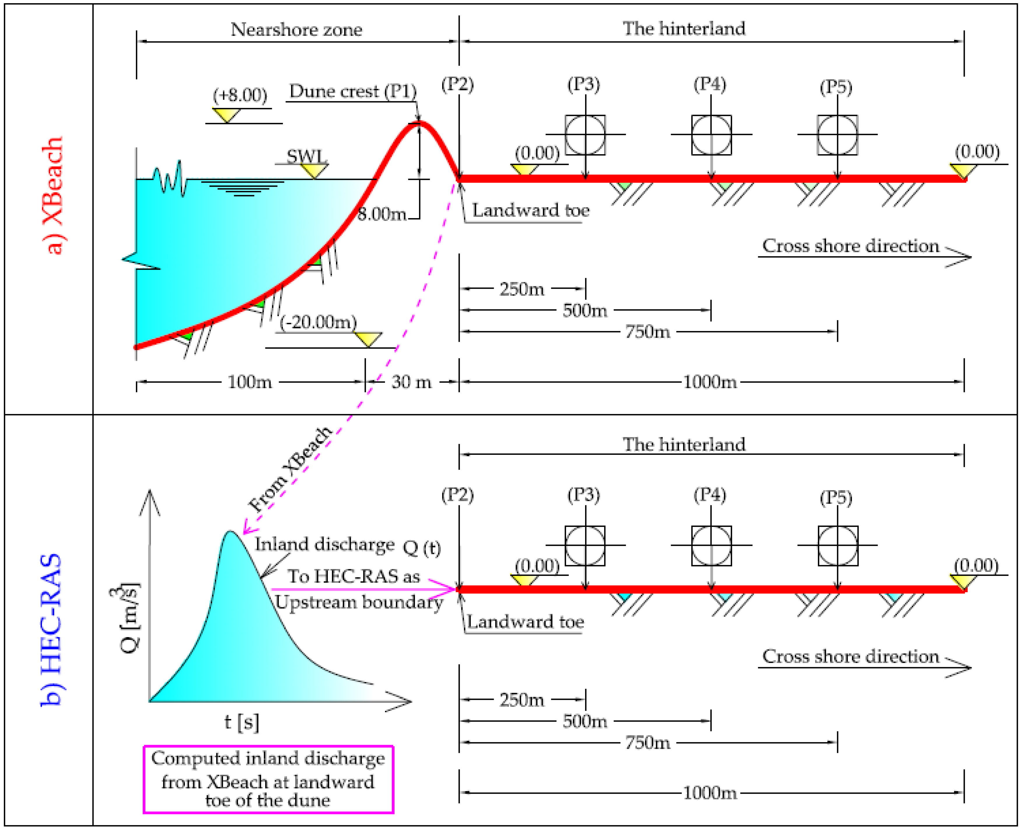
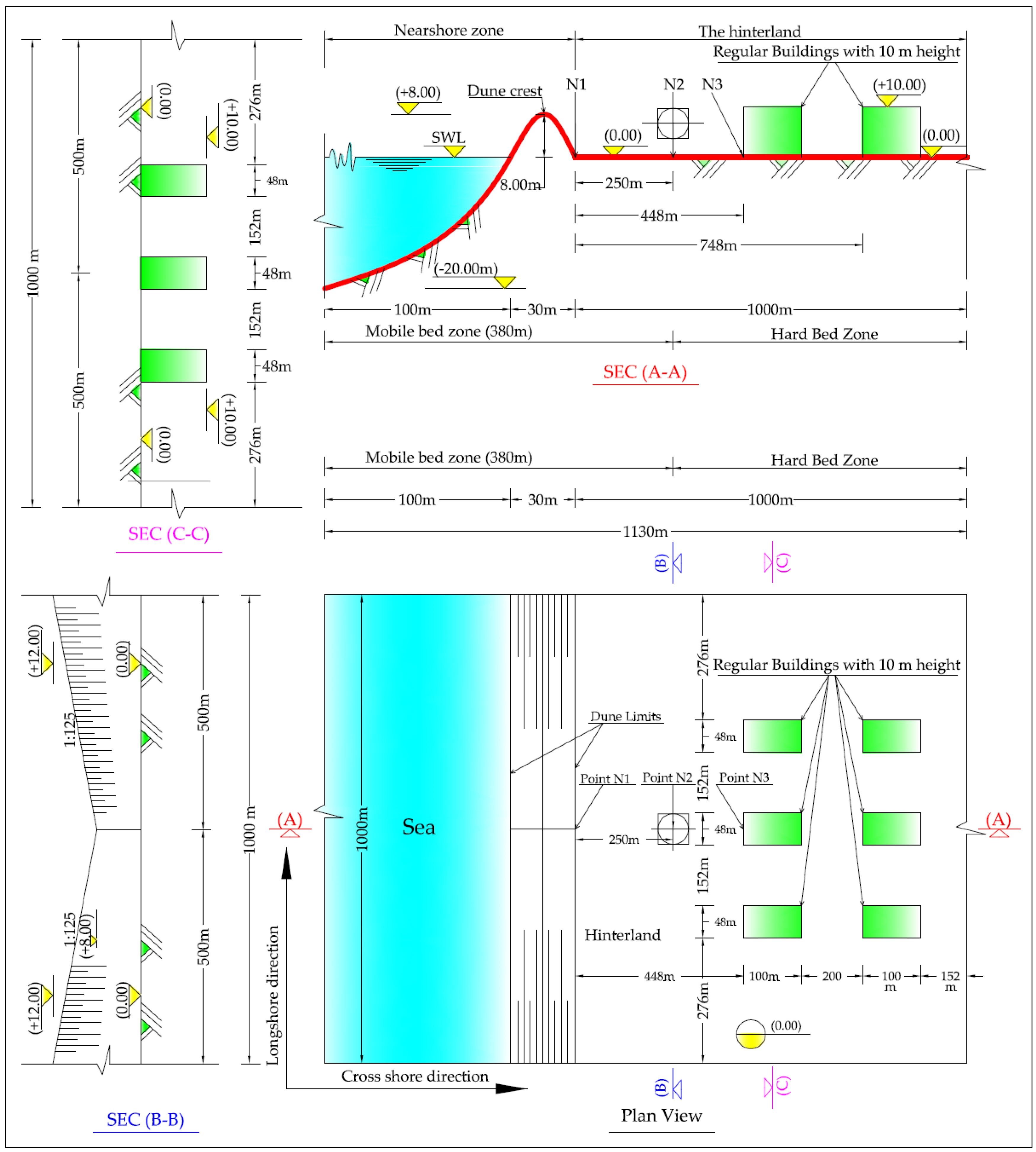
3.1. 1D Synthetic Cross-Shore Profile

In order to validate first the 1D version of XBeach for the proposed combined modelling of the overtopping/overwash and the induced coastal flooding, the synthetic cross-shore profile in Figure 1a is considered. For this purpose, XBeach is applied in the nearshore seaward of the dune toe to obtain the time-dependent inland discharge Q(t) at the landward toe of the dune which is used as an upstream boundary condition for the 1D inundation model HEC-RAS (Figure 1b) that is limited to the hinterland only. The results obtained from XBeach applied as a 1D inundation model in the hinterland are finally compared to the outcomes from HEC-RAS.

The cross-shore profile in Figure 1a represents a numerical waveflume with a width of 5.0 m (alongshore) and a length of 1130 m. The cross-shore profile consists of three main cross-shore stretches: a 100 m sea stretch, a 30 m sandy dune stretch and 1000 m hinterland stretch, where the dimensions and levels of each stretch are shown in Figure 1 (not to scale). In the sea stretch, the bed level varies from −20.00 m at offshore to 0.00 at the shoreline. The base width and the height of the dune are, 30.0 m and 8.0 m, respectively, where the height is measured from zero sea water level SWL (Mean SWL) as a datum. A 1.0 km flat stretch is added to the landward toe of the dune to represent the profile extent in the hinterland. The main parameters and boundary conditions used within XBeach to simulate this profile are shown in

Table 1. Main parameters and boundary conditions used in the analysis of the 1D synthetic profile (Figure 1a) using XBeach.

Parameter	Value	Meaning	Note
D50	2 mm	Median grain size
dx	2 m	Cross-shore spatial step	Regular spatial step
dy	5 m	Profile width
Bedfriction	n	Manning parameter (selected as representative for the bed friction)
bedfriccoef	0.03 m-1/3·s	Value of Manning coefficient	This value is generalised over the whole model
instat	4 or jons	Standard Joint North Sea Wave Project (JONSWAP) JONSWAP spectrum is selected as an upstream wave boundary condition	The selected spectrum coefficients are: Hs (significant wave height) = 1.5 m and Tp (peak period) = 6.6 s
front	0	Absorbing–generating weakly-reflective boundary is used as a 1D inflow boundary
back	1	Absorbing–generating weakly-reflective boundary is used as a 1D outflow boundary
left	1	Impermeable wall is a lateral flow boundary	Left side wall of the numerical wave flume
right	1	Impermeable wall is a lateral flow boundary	Right side wall of the numerical wave flume
lateralwave	Neumann	Neumann boundary is a lateral wave boundary in both lateral sides	The alongshore gradient of the wave energy is zero at the lateral boundaries
asabeta	11.30	Average slope angle accounts for the beach slope effect on wave nonlinearity	See Elsayed and Oumeraci, (2016 [39])
facpi	1	Grain-stabilization effect is not considered	See Elsayed and Oumeraci, (2016 [39])
form	2	Sediment transport is calculated according to Van Thiel–Van Rijn formulation	See Roelvink et al. (2015 [52])
tstop	3600 s	Simulation time
tint	1 s	Output time step

, while all other XBeach parameters (see Roelvink et al. 2015 [52]) are kept by the default of XBeach.

The bed is considered non-erodible (hard bed) in the hinterland stretch and erodible from the landward toe of the dune to offshore (“nearshore zone”), with a median grain size of 2 mm. The cross-shore spatial step (dx) is considered regular at 2 m length. For both the coastal zone and the hinterland, a Manning coefficient n = 0.03 [$m^{-1/3}·s$] is assumed to account for bed friction. The storm-induced waves (low-frequency waves) are represented by a Joint North Sea Wave Project (JONSWAP) spectrum with Hs = 1.5 m (significant wave height) and Tp = 6.6 s (peak period). Moreover, the wave direction is considered perpendicular to the coastline while the water flow outside the hinterland stretch in the downstream direction is permitted.

During a storm surge event of 1.0 h, it is assumed that the SWL rises from level zero (0.00 m) as a long wave resulting from the combination of both surge and astronomical tide effects. Two scenarios for the formation of this long wave are considered, where each scenario represents a hydraulic load case (Figure 2):

(i)

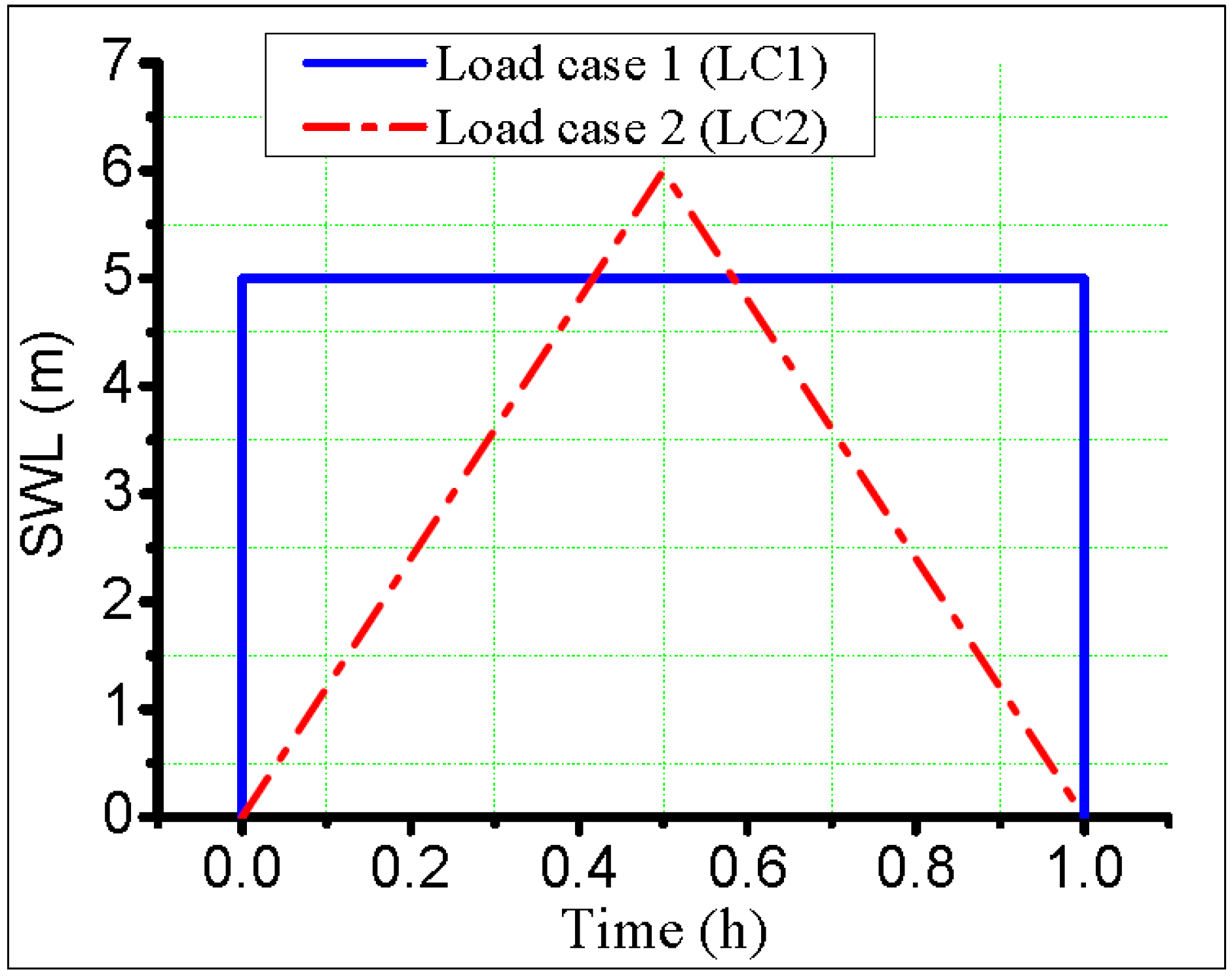
Load case 1 (LC1): represents, in addition to the wave action described by a JONSWAP spectrum, a sudden sea level rise from 0.00 m to +5.00 m where the latter level persists over the entire storm duration (rectangular shape) and

(ii)

Load case 2 (LC2): represents, in addition to the wave action described by a JONSWAP spectrum, a linear sea level rise from 0.00 m to 6.00 m within half of the storm duration followed by a linear decrease at the same rate to level 0.00 m within the other half (triangular shape).

The hinterland stretch (Figure 1b) is modelled in HEC-RAS using the inland discharge of water and sediment calculated from XBeach at the landward toe of the dune as upstream boundaries. In addition, the same modelling conditions of the synthetic profile by XBeach are considered in the HEC-RAS model. For instance, the lateral flow is prevented by impermeable walls and levee boundaries (boundaries to prevent the lateral flow) in both XBeach and HEC-RAS models, respectively. Moreover, five measuring points (P1–P5), as shown in Figure 1, are set as reference points in the XBeach model while three of them (P3–P5) are considered for comparison of the outcomes from XBeach and HEC-RAS. The results of this comparison are presented in Section 4.1.

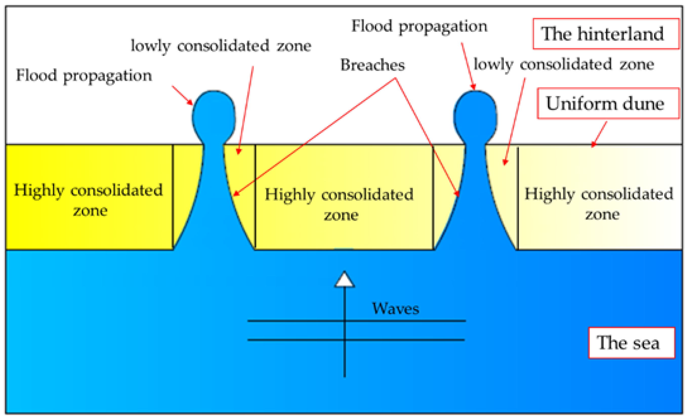
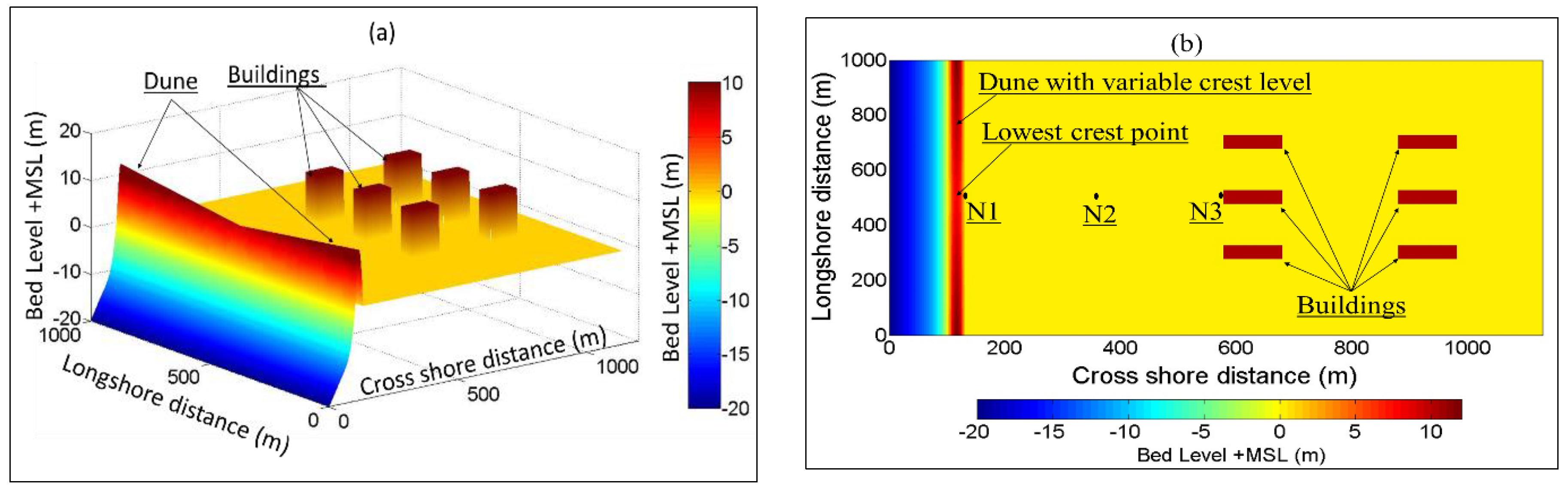
3.2. 2D Synthetic Coastal Zone

The coastal zone (1130 × 1000 m) in Figure 3 (all dimensions and levels are set in metres and not to scale) represents a synthetic two-dimensional horizontal (2DH) case study. This zone is also divided into three main stretches as described above. In the 100 m sea stretch, the bed level varies from −20.00 m at offshore to 0.00 m at the shoreline. The dune has a fixed base width of 30 m, while the crest level varies linearly in the longshore direction from level +8.00 m at the dune centre to level +12.00 m at the lateral edges of the considered zone, i.e., the dune crest and thus its side slopes vary alongshore. This longshore variability of the dune dimensions is assumed in order to attempt getting a breach initiation at the lowest point of the dune crest. The hinterland is considered flat and horizontal with a 0.00 m-bed level. However, it contains six regular buildings of 10 m height and horizontal dimensions of 100 × 48 m. These buildings are set in order to check the capability of XBeach to simulate building effects on the flood propagation.

Three points, N1, N2, and N3, as shown in Figure 3, are set as reference points in the XBeach model. Moreover, three cross-sections are provided in Figure 3 to illustrate the details of the considered coastal area: the first is Sec A-A that passes through the lowest crest of the dune and thus the mid of two buildings, while the second and third cross-sections are alongshore sections that pass, respectively, through the measuring point N2 (Sec B-B) and through the middle of the first seaside row of the buildings (Sec C-C).

The bed is considered erodible in both sea and dune stretches. Moreover, a stretch of 250 m of the hinterland adjacent to the dune is also considered erodible, while the rest of the hinterland is considered non-erodible (Hard bed as shown in Figure 3). Because the buildings are simulated in XBeach as ground elevations, the bed in the building zone and the buildings themselves are considered non-erodible. For the mobile bed zones, a median grain size of 2 mm is assumed. The bed friction is set by using an assumed Manning coefficient n = 0.03 [$m^{-1/3}·s$], which is considered uniform over the entire model.

Similar to the hydraulic loads in the previous synthetic case (Section 3.1), the wave direction is considered perpendicular to the coastline and the storm-induced waves are represented through the model by a JONSWAP spectrum with Hs = 1.5 m and Tp = 6.6 s. The JONSWAP option in XBeach generates alongshore varying time series of the wave energy on the basis of a specified analytical 2D JONSWAP-type spectrum. As a result, the JONSWAP spectrum imposes XBeach to stochastically generate short-crested waves, with variable wave height in the longshore direction. The longshore variability of the wave height (or generally the longshore variability of the hydraulic load) means alongshore varying wave impact (wave collision by breaking waves), alongshore varying wave run-up and rundown, and accordingly alongshore varying erosion. During a storm surge event of 1.0 h, it is assumed that the SWL rises from zero level (0.00 m) as a long wave resulting from the combination of both surge and astronomical tide effects. The formation of the sea level is assumed to take the rectangular form shown in Figure 2. The whole zone in Figure 3 is simulated in XBeach considering the same parameters and boundary conditions in Table 1 except those shown in

Table 2. Main parameters and boundary conditions used in the analysis of the 2D synthetic coastal area (Figure 3) using Xbeach.

Parameter	Value	Meaning	Note
front	1	Absorbing–generating weakly-reflective boundary is used as a 2D inflow boundary
left	0	Neumann boundary is a lateral flow boundary	Neumann means that gradient of the lateral outflow is zero
right	0	Neumann boundary is a lateral flow boundary
back	2	Absorbing–generating weakly-reflective boundary is used as a 2D outflow boundary
lateralwave	Neumann	Neumann boundary is a lateral wave boundary in both lateral sides of the model
dy	2 m	The spatial step in the longshore direction	Regular spatial step
morfac	10	Factor in Exner equation to accelerate the calculations of the morphological evolution	See Roelvink et al. (2015 [52])
tstop	5400 s	Simulation time
tint	5 s	Output time step

.

The flood propagation in the hinterland zone is simulated in River-2D over a calculation mesh containing the topography of the hinterland only and considering the inland discharge through the expected breach (es), computed from XBeach as inflow boundary. The grid of the River-2D model is designed so that the distance between the TIN nodes is in the range from 8 m to 12 m. The former lower limit (8 m) is chosen to avoid model instabilities during high flow velocity regimes, while the latter (12 m) is chosen so that four nodes can be generated along the shorter dimension (48 m) of the buildings in Figure 3. In order to compare the flood extent and kinematics in the hinterland, the same simulation circumstances of XBeach are applied to the River-2D model. For instance, water outflow outside the hinterland zone in downstream and lateral directions is permitted where Neumann lateral flow boundaries are considered. Moreover, the same constant values for bed friction (n = 0.03 [$m^{-1/3}·s$]) and eddy viscosity (${\nu }_h=$ 0.1 [$m^2/s$]) are applied in both XBeach and River-2D models. The results of this comparison are shown in Section 4.2.

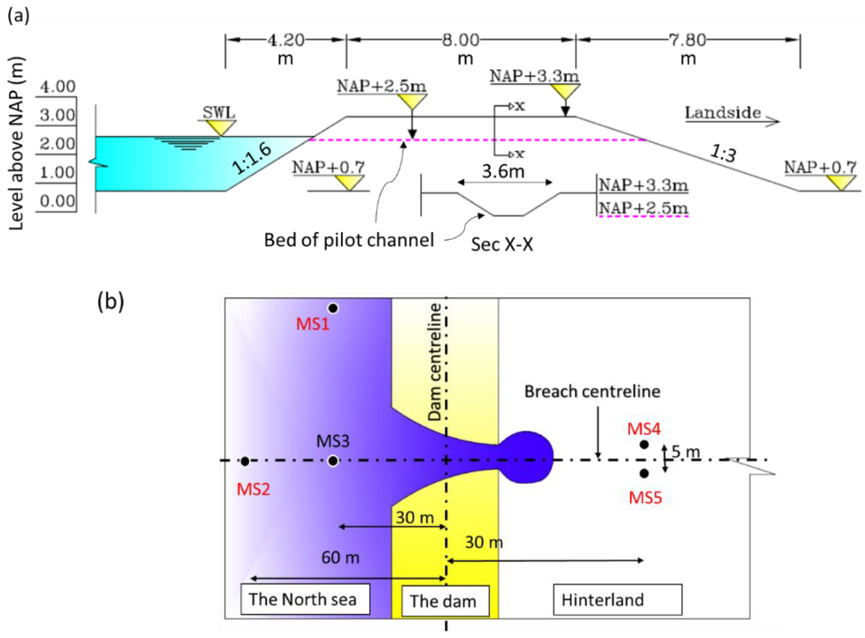
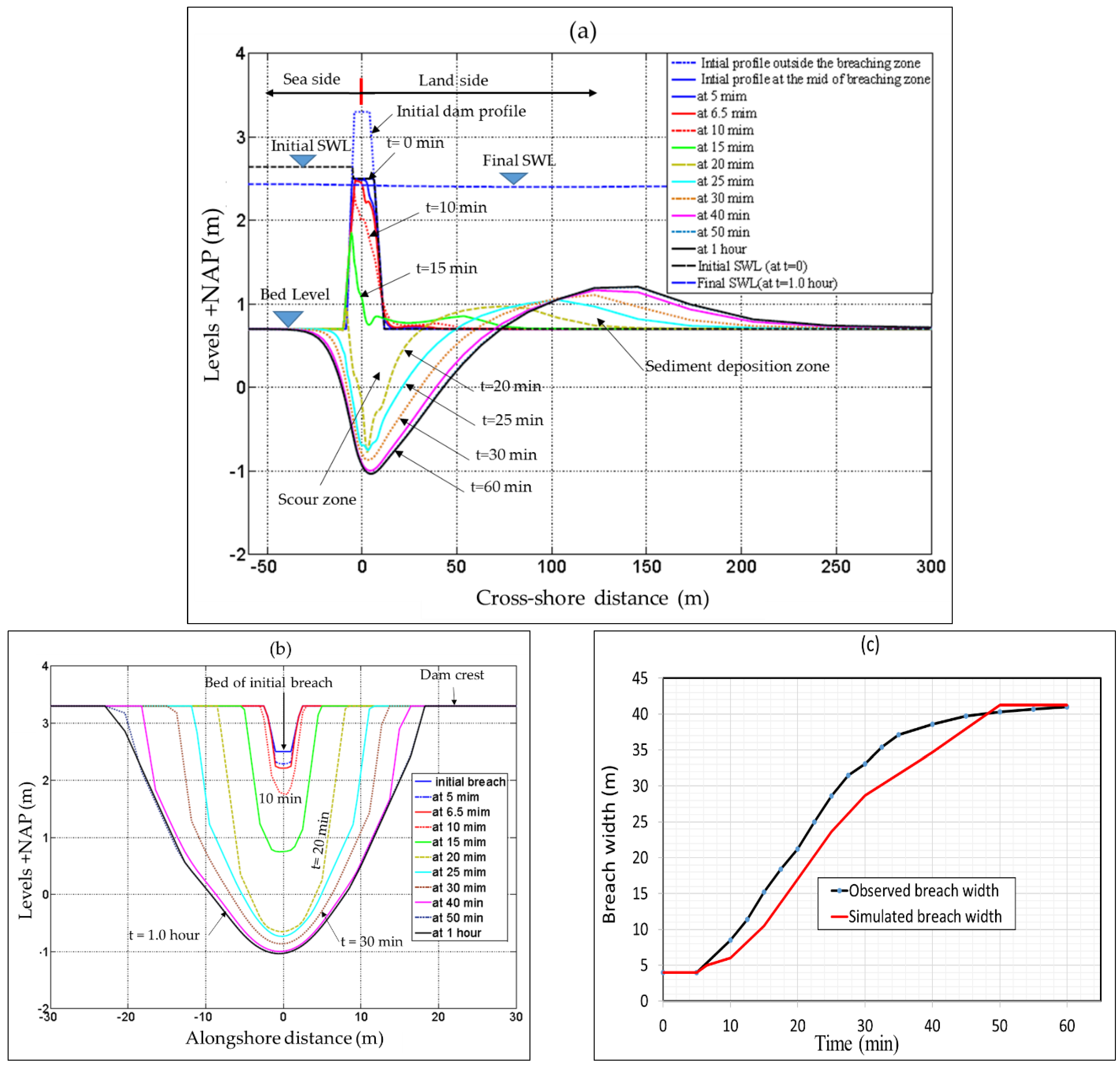
3.3. The Case of Het Zwin

In the mouth of the Zwin, a tidal inlet located at the border between the Netherlands and Belgium, an artificial dam (Figure 4a) was constructed in 1994 with a crest height of 3.3 m + NAP (Dutch datum), crest width of 8 m, landward slope of 1:3, seaward slope of 1:1.6 and longshore length of 250 m. The mean tidal range at Zwin is around 2.85 m. Therefore, the mean tidal prism of the Zwin is about $350,000 m^3$. The dam was constructed in order to perform an overtopping-induced breaching test to validate the breaching model BRES (Dutch for breach) of Visser (1998 [64]). Therefore, the breach width at the crest was the main measure. The test is well documented in Dutch by Bakker et al. (1996 [65]) and in English by Visser (1998 [64]).

To ensure that the breach is initiated at a certain location, an initial breach was enforced in the middle of the dam (Sec X-X in Figure 4a) having a depth of 0.8 m, a bed width of 1 m and side slopes of 1:1.6. The level of the surrounding seabed was about 0.7 m + NAP and the experiment was performed under calm conditions (i.e., no waves and no wind). Therefore, the water elevation was the main driver for the breaching process. As a result, the breach developed to a width of 41 m within one hour after the breach initiation. In addition to measuring the temporal evolution of the breach width, the water levels above the NAP and flow velocities were also measured during the experiment at both up- and downstream the dam using five measuring stations MS1 to MS5 (Figure 4b).

Considering the model dimensions in Figure 4, the Zwin dam test was reproduced in XBeach by Roelvink et al. (2009 [23]), using a non-uniform grid with grid sizes gradually varying from 0.5 m near the breach to approximately 50 m far away from it. The median grain diameter $D_{50}$ of the bed material was set to 0.3 mm in accordance with the prototype test conditions for the artificial dam. In order to achieve the same volume of the tidal prism, Roelvink et al. (2009 [23]) defined the volume of the tidal prism using a prismatic profile, so that the mean tidal prism remains the same (350,000 $m^3$). Though the experiment was performed under calm conditions and though the tidal prism is replaced by an equivalent prism, this experiment is still appropriate to validate the application of XBeach for the proposed combined modelling of breaching and the induced flood propagation based on:

(i)

The comparison between the observed and calculated breach widths to assess the capability of XBeach as a breaching model.

(ii)

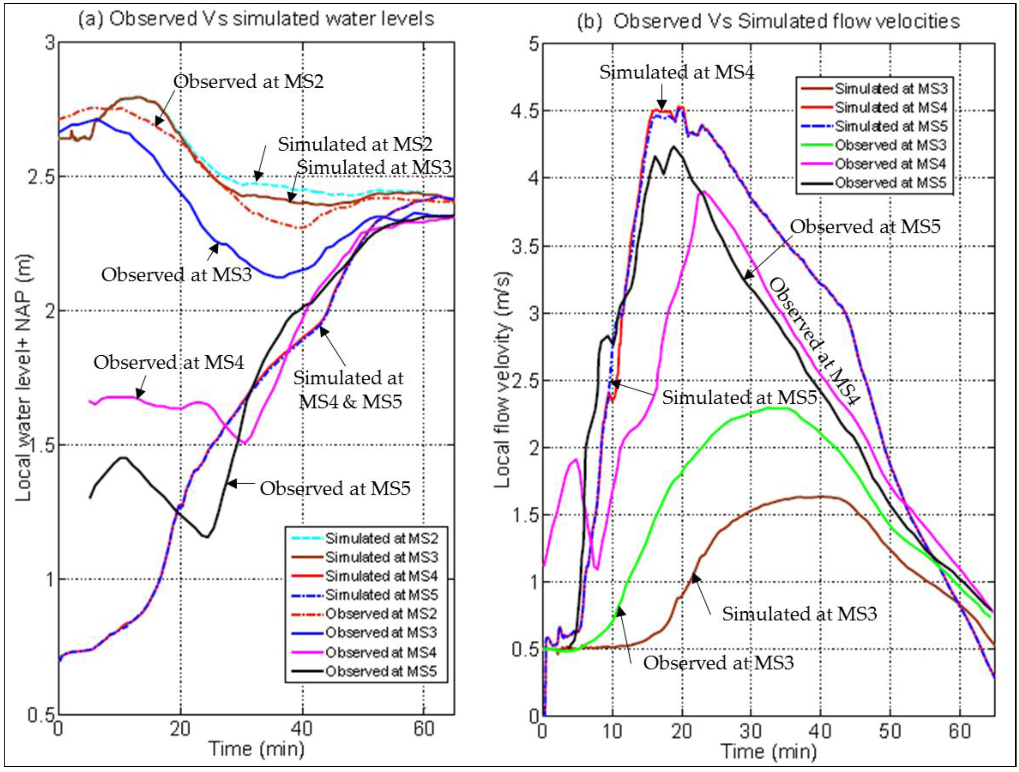
The comparison between the observed and modelled water depths and flow velocities at the measuring stations MS4 and MS5 (located behind the dam) to show that XBeach correctly calculates the water depths and flow velocities in the hinterland.

(iii)

The comparison between the volume of the tidal prism and the total inflow discharge to prove that XBeach calculates the flood extent correctly.

The breaching model of Roelvink et al. (2009 [23]) is run again using the default setting in addition to the model settings in

Table 3. Main parameters used in the analysis of the breach and the induced flooding at Het Zwin using XBeach.

Parameter	Value	Meaning	Note
facpi	1.3	Grain-stabilization effect is considered by increasing the critical stirring velocity by 30%	See Elsayed and Oumeraci, (2016 [39])
form	2	Sediment transport is calculated according to Van Thiel–Van Rijn formulation	See Roelvink et al. (2015 [52])

, which represent the difference between this simulation and Roelvink’s simulation. The validation results are presented in Section 4.3.

4. Results

The results of the first test case are presented in Section 4.1, while Section 4.2 describes the results of the second test case. The results of the dam breach at Het Zwin are then presented in Section 4.3.

4.1. 1D Synthetic Cross-Shore Profile

The synthetic profile in Figure 1.a is simulated in XBeach under both the rectangular (LC1) and triangular (LC2) loads as described in Figure 2. The results of these simulations are presented in Section 4.1.1 and Section 4.1.2, respectively. As a result, the inland discharges of both water and sediment are calculated in Section 4.1.3 at the dune’s landward toe. The latter discharges are used as upstream boundary conditions for the inundation model HEC-RAS by considering only the hinterland in Section 4.1.4. As a result, the computed water levels and flow velocities by both XBeach and HEC-RAS are compared.

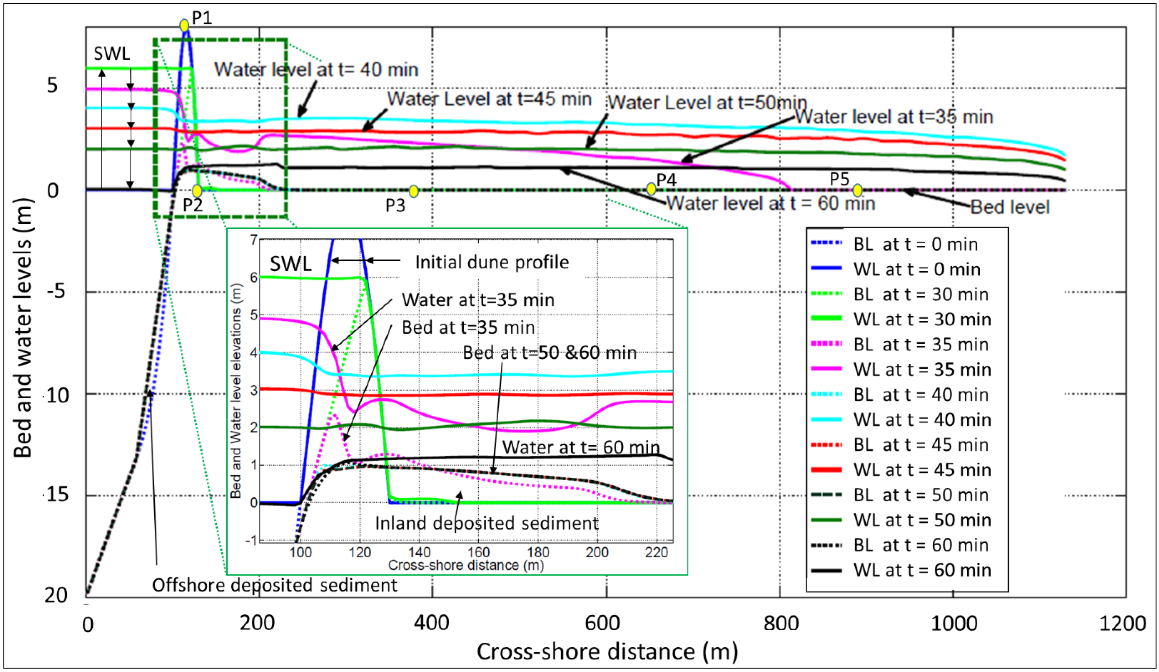
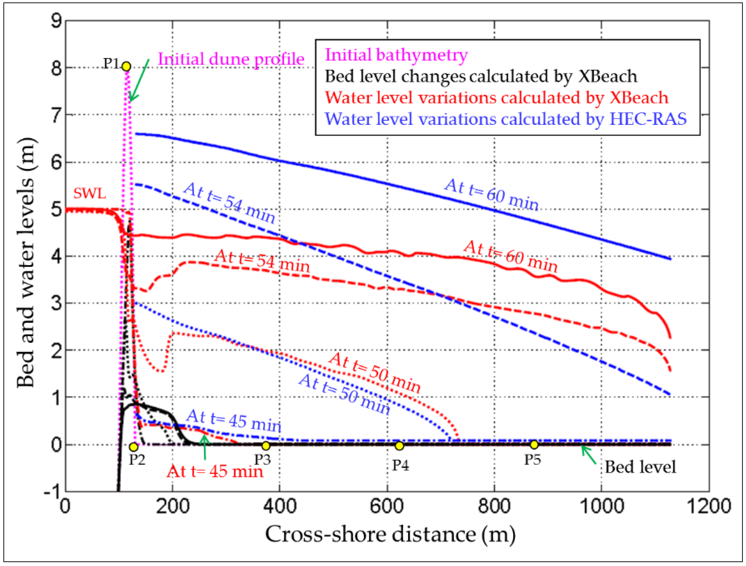
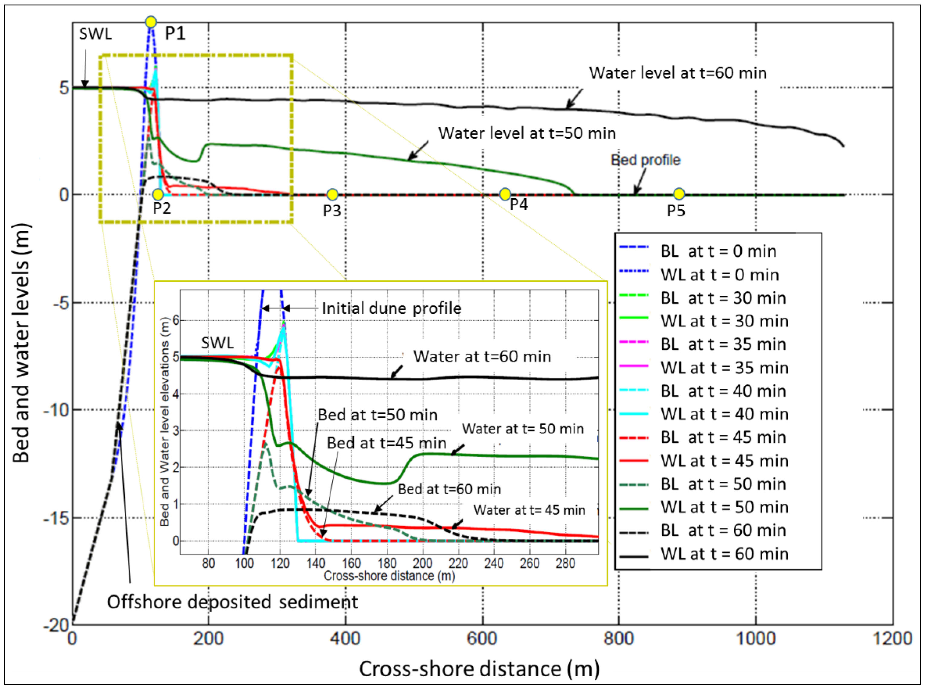
4.1.1. Bed Profile and Water Level Evolution under Load Case LC1 by XBeach

Under load case 1 (rectangular evolution of sea level with wave action) as defined in Figure 2, the dune is totally overwashed so that seawater can propagate into the hinterland. Figure 5 shows the evolution of both bed level and water level in both sea and hinterland.

A seaward erosion of the dune, which is accompanied by a seaward avalanching, is observed. It develops up to 30 min, resulting in a progressive lowering of the dune crest from level +8.00 m at the start of the simulation to level +6.00 m, which means that the dune was under the collision regime of Sallenger (2000 [66]); i.e., a regime during extreme events, at which the frontal seaward face of a coastal barrier is subject to collision by breaking waves as well as to wave runup and rundown. The eroded sediment transported under the rundown effect deposits offshore. Because of the dune crest lowering during the first 30 min to level +6.00 m, the sea waves overtop the dune, causing landward erosion. The overtopping phase extended over a duration of ca. 15 min (from 30 min to 45 min). During this phase, the dune crest is lowered ca. 1 m more, thus allowing seawater to overflow the eroded dune. The overflow phase extended until the simulation end, where significant morphological changes occurred during this phase, resulting in full damage of the dune and in sediment deposition behind the dune. As a result, a significant amount of seawater flows inland inducing hinterland flooding. For both overtopping and overflow regimes, the dune works like a broad-crested weir with a movable crest, where a free flow (i.e., no backwater effect) is noticed during the overtopping phase and the beginning of the overflow phase. This movable crest weir becomes submerged with the time marching, which results in the formation of a hydraulic jump downstream of the dune (see the water surface at t = 50 min in Figure 5). The hydraulic jump indicates the flow transition from supercritical flow over the dune (Froude number >1) to subcritical flow (Froude number <1) behind it. The length of the hydraulic jump varies with the height of the dune and vanishes when the water level in the hinterland (behind the dune) becomes almost equal to the SWL.

4.1.2. Bed Profile and Water Level Evolution under Load Case LC2 by XBeach

The difference with LC1 (rectangular) is the variation of the SWL, which for LC2 (triangular) is linearly increased from level 0.00 m to level +6.00 m within 30 min and then linearly decreased at the same rate to level 0.00 m after 1.0 h (see Figure 2). Figure 6 shows the evolution of both bed and water levels under LC2.

Similar to the behaviour under the rectangular load case, seaward erosion is preliminarily developed resulting in dune crest lowering. Such lowering is followed by wave overtopping at approximately 27.5 min. At this time, both the SWL and dune crest are approximately at the same level. However, the waves overtop the dune followed by overflow. During overflow, the dune behaves like a broad-crested weir, resulting in a supercritical flow over the dune and a subcritical flow behind it. Between these two flow regimes, a hydraulic jump is visible from the water level at t = 35 min (Figure 6). With the time marching (from t = 40 min onwards), the dune behaves like a submerged weir. However, the decrease of the SWL reduces the difference between the water levels in front of and behind the dune and thus the inland flow velocity decreases and the hydraulic jump vanishes. Moreover, the SWL becomes lower than the water level in the hinterland at the end of the simulation time. However, the overwash and inundation processes, in general, are faster under the triangular load case (LC2) than under the rectangular one, which means that the form of the hydraulic load affects the speed of both the erosion and the inundation processes.

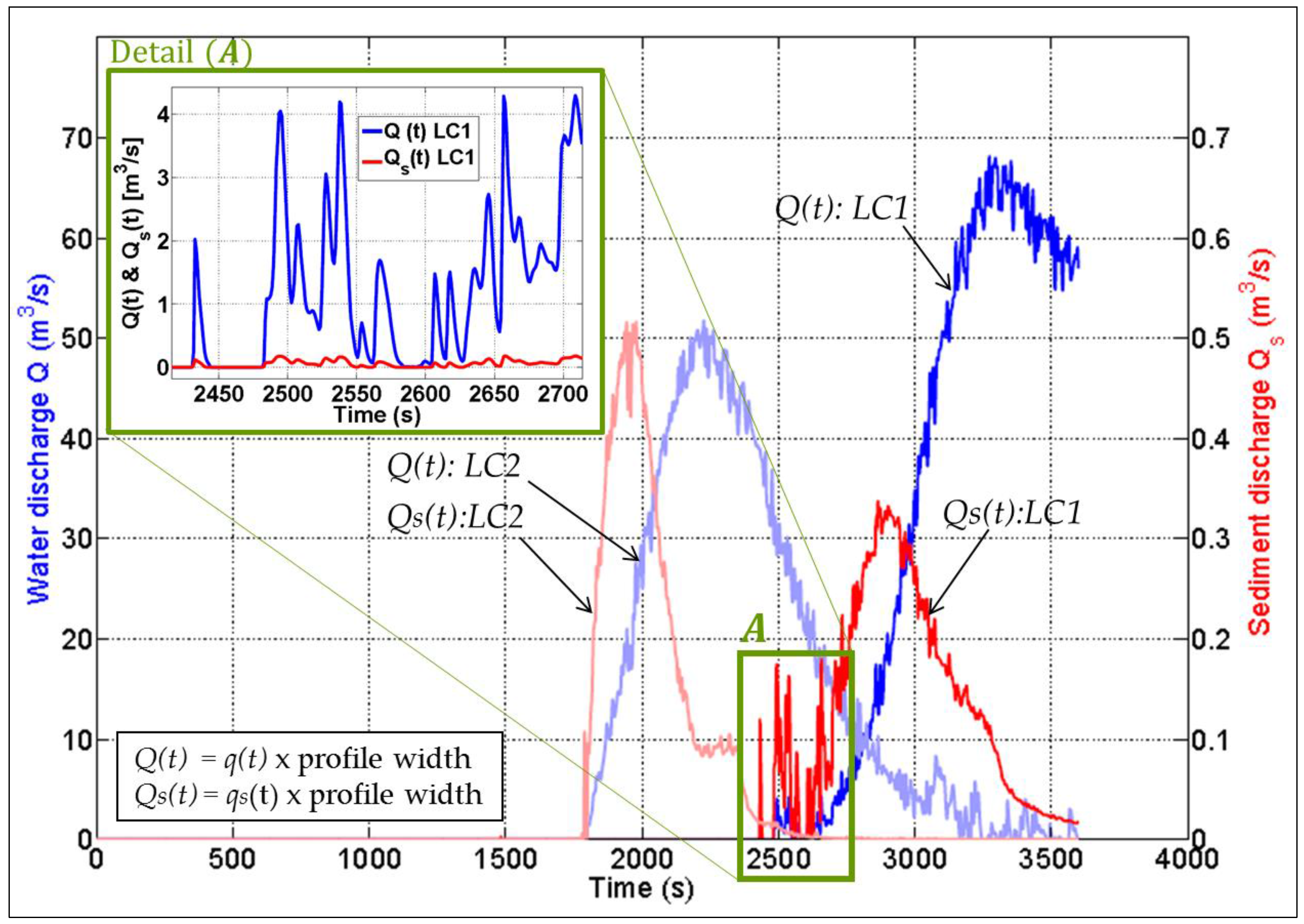
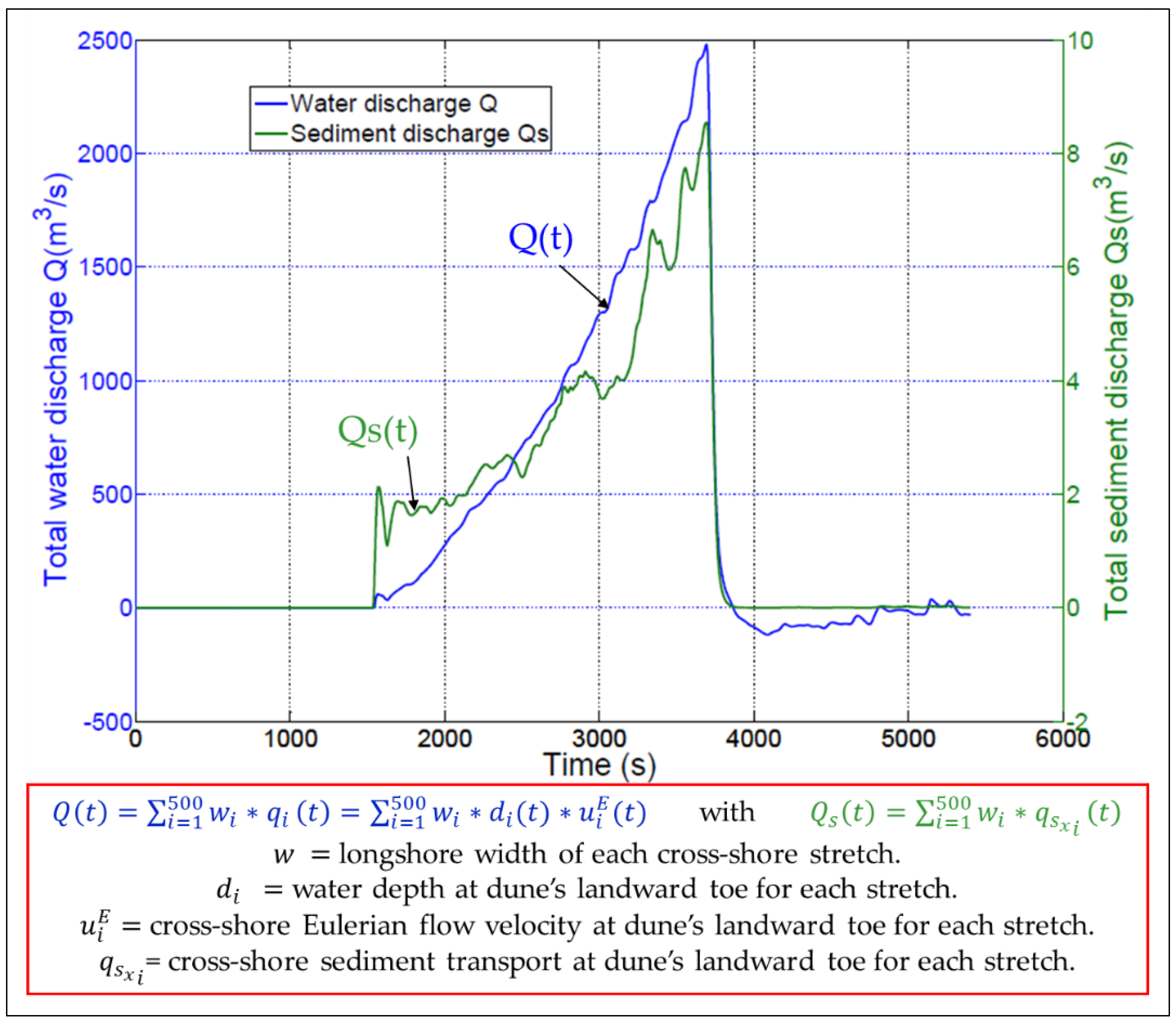
4.1.3. Water and Sediment Inflow Discharges to the Hinterland

Though the XBeach model does not provide a direct estimation of the inland flow rate, the outputs can be exploited to calculate the flow rate over the crest of a coastal barrier and/or through a breach induced inlet. The inland discharge per meter q(t) over the dune can simply be calculated at either the barrier crest or at the landward toe of a barrier (e.g., P1 and P2 in Figure 6 or Figure 7, respectively) using the products of the Eulerian velocity vector $u^E\left(t\right)$ at these locations and the local water depth vector $d\left(t\right)$ at the same locations. However, the inland discharge calculation at the dune crest (i.e., at P1) is not favoured due to the high mobility (erosion) of the dune crest. In fact, the seaward avalanching results in a lowering of P1 until it falls under the collision regime. In such a situation, discharges at the point P1 are often counted by negative values as long as P1 has fallen beneath wave run-down. During wave rundown, the Eulerian velocity and the discharge are directed offshore and thus have negative values. Such negative values must be avoided when passing the inland discharge to another propagation model (e.g., HEC-RAS) to be used as an upstream boundary for the flood propagation in the hinterland by such models. Therefore, calculating the inland discharge at the landward toe (e.g., at P2) is preferred. Figure 7 shows a comparison between the computed inland water and sediment discharges under both load cases LC1 and LC2.

The erosion process and thus the induced hinterland inundation take place earlier under the triangular load case LC2 (inundation start at t ≈ 1650 s = 27.5 min) than under the rectangular load case LC1 (inundation start at t ≈ 2400 s = 30 min). However, the peak discharge is higher under LC1 than LC2. On the contrary, the sediment discharge under LC2 has a higher peak as compared to LC1. Moreover, the ratio between the sediment to water inflows under LC2 is almost 1%. This ratio decreases under LC1 because more sediment is directed offshore during the collision regime under LC1 than under LC2.

Figure 7, in addition, shows that the sediment transport peaks precede the flow peaks under both LC1 and LC2. The sediment transport potential depends, in addition to the sediment characteristics, on the bed shear stress, which is higher as long as both the discharge and the steepness of the landward slope of the dune are sufficiently high. Therefore, the steeper slope of the dune landward face at the beginning of the overtopping is associated with higher gravity forces on the sediment, so that a lower water discharge Q is required for sediment mobility and transport. This additional gravity effect is higher on the sediment than on water (due to density difference) and might thus result in higher sediment discharge as compared to those under the effect of the peak water discharge. As a result, the sediment discharge peak (i.e., the peak of the sediment transport potential) develops earlier than the water discharge peak. These rather counter-intuitive results are consistent with the result of Worni et al. (2014 [30]), who compared the temporal evolution of the water discharge with that of the bed shear stress during the entire breaching process. In fact, their comparison shows that the peak of the latter occurs before the water discharge peak. When the overwash progresses, the steepness of the dune landward slope decreases (see Figure 5 and Figure 6) and the sediment transport potential decreases accordingly. On the other hand, the flow peak is reached, especially in these weir-like cases, when the sea level over the dune crest reaches its maximum. The latter condition might be achieved at a later stage of the overtopping process when the slope of the dune landward face becomes milder. At this stage, the sediment discharge is lower as compared to that at the beginning of the overtopping. Therefore, the water discharge peak might be reached later than the peak of the sediment discharge as shown in Figure 7. In the case of a breach, the lateral feeding of the sediment by avalanching from the lateral sides of the breach-induced channel would result in inseparable water and sediment peaks as depicted in Figure 14.

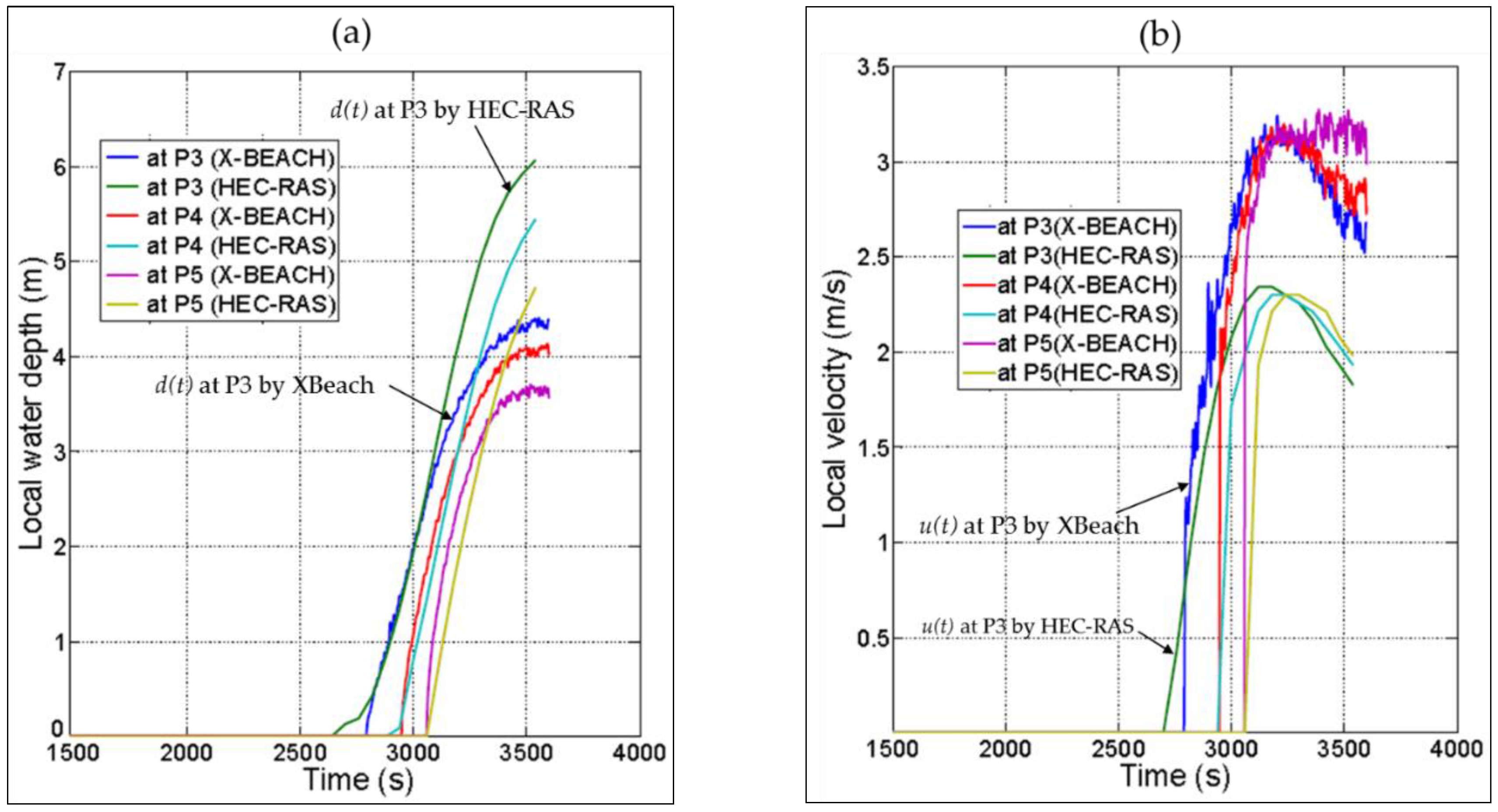
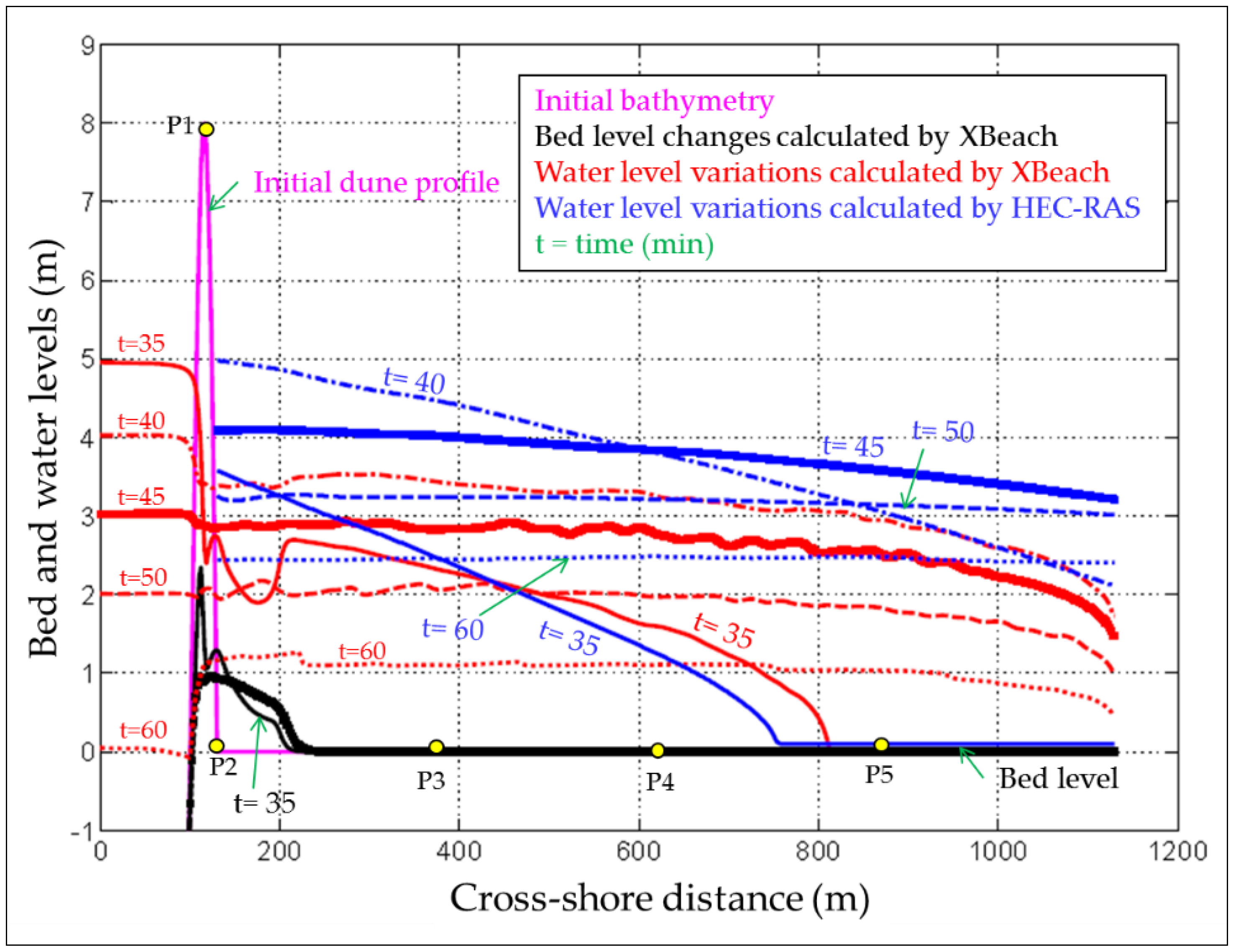
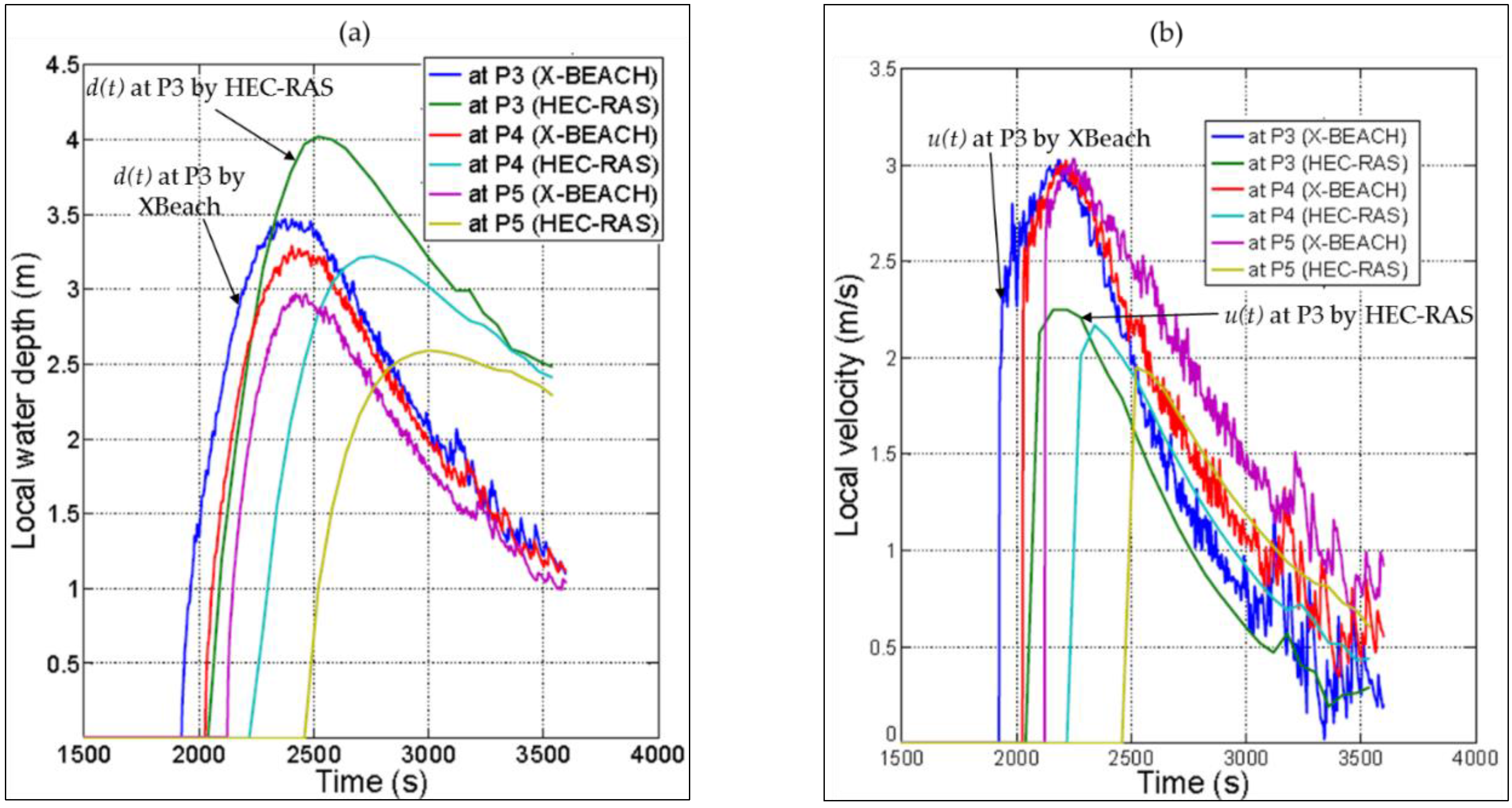
4.1.4. Comparison of Inundation Depths and Velocities Obtained from XBeach and HEC-RAS

The HEC-RAS model is used as a benchmarking inundation model to compare the obtained hinterland inundation against the one by XBeach. The same model set-up (e.g., bed friction) and boundary conditions are applied in the HEC-RAS model as in XBeach (see Elsayed and Oumeraci, 2016 [66] for further details). Moreover, both the water and sediment discharges in Figure 7 are used as upstream boundaries to the HEC-RAS model. The sediment transport in the HEC-RAS model is calculated using the formula of Meyer-Peter–Muller (Meyer-Peter and Muller, 1948 [49]). As a result, a comparison of the temporal evolution of water profiles in the hinterland stretch by both HEC-RAS and XBeach are shown in Figure 8 and Figure 9 for the rectangular and triangular load cases, respectively.

In Figure 8, the water levels at times 45 and 50 min from both HEC-RAS and XBeach are almost convergent, thus providing a first indication of the capability of XBeach applied as an inundation model. However, HEC-RAS provides higher water levels at times 54 and 60 min, where the difference is larger upstream than downstream of the hinterland stretch. The higher water levels by HEC-RAS at the hinterland inlet can be attributed to the effect of the upstream boundary. In fact, mass conservation is fulfilled, when feeding HEC-RAS by the inflow hydrographs computed from XBeach, but the momentum conservation principle is omitted; i.e., the inland discharge alone is not enough as an inflow boundary condition for HEC-RAS. In addition, the variation of the flow velocity at the hinterland inlet would also be required, so that the model could correctly calculate the water level at the hinterland inlet based on both the imposed hydrograph and flow velocity. Since there is no possibility to feed the inland velocity to HEC-RAS, it calculates the water level at the model inlet based on the incoming discharge and the local bed slope. As a result, with this flat and horizontal bed, HEC-RAS assumes that the flow at the hinterland inlet is always subcritical, which is only appropriate at the beginning of the inundation. The latter might explain why the water levels converge at times 45 and 50 min. At the beginning of the overflow phase, the flow over the dune and at P2 is supercritical, while it is subcritical according to HEC-RAS. This might explain why HEC-RAS provides higher water levels at times 54 and 60 min. The higher water depth at the hinterland inlet results in providing lower values for the associated flow velocity. As a result, the HEC-RAS model cannot reproduce the hydraulic jump at the model inlet. The higher water depth at the inlet leads to a general increase of the water depths, as well as a general decrease of the flow velocity at the points P3, P4 and P5 as shown in Figure 10.

Similarly, the water levels in Figure 9 under LC2 provide the same behaviour as under LC1. At 35 min, the water levels are convergent since the upstream boundary does not yet have a significant effect. Afterwards, HEC-RAS provides higher water levels due to the effect of the upstream boundary. Figure 11 also shows the temporal evolutions of the water depths and velocities at the measuring points P3, P4 and P5 under LC2.

In Figure 10 and Figure 11, the water depths from HEC-RAS and XBeach increase at the same rate at the inundation start, but the increasing rates from XBeach become lower than those from HEC-RAS by 30% to 40% due to the upstream boundary effect in which the difference increases at the nearer points to the upstream boundary. The higher increase of the water depths in HEC-RAS, as compared to those in XBeach, may explain why the depth-averaged velocities from HEC-RAS are lower than those from XBeach by 30% to 40%.

4.2. 2D Synthetic Coastal Zone

The synthetic study case in Figure 3 is simulated in XBeach under load case LC1 as defined in Figure 2. The results of the breach and flood propagation simulation are analysed in Section 4.2.1. The water and sediment inflow discharges to the hinterland are obtained in Section 4.2.2. Consequently, the water discharge is used as an upstream boundary condition for the inundation model River-2D, including only the topography of the hinterland in Section 4.2.3, so that the performance of XBeach in the hinterland can be examined by comparing its outcomes with River-2D outcomes.

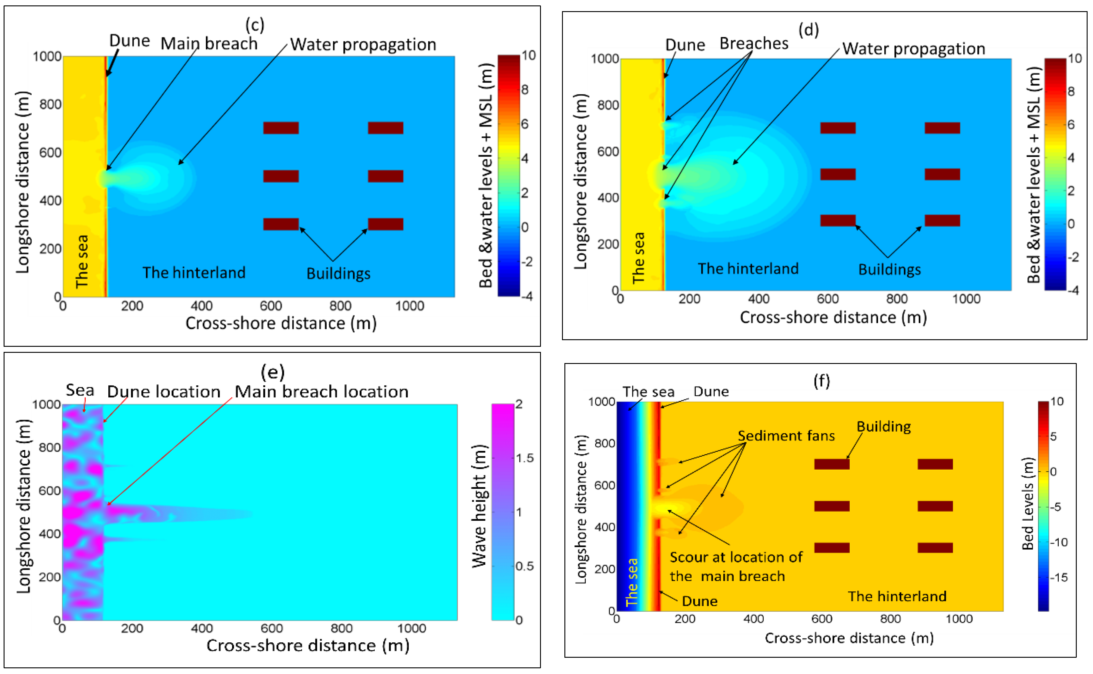
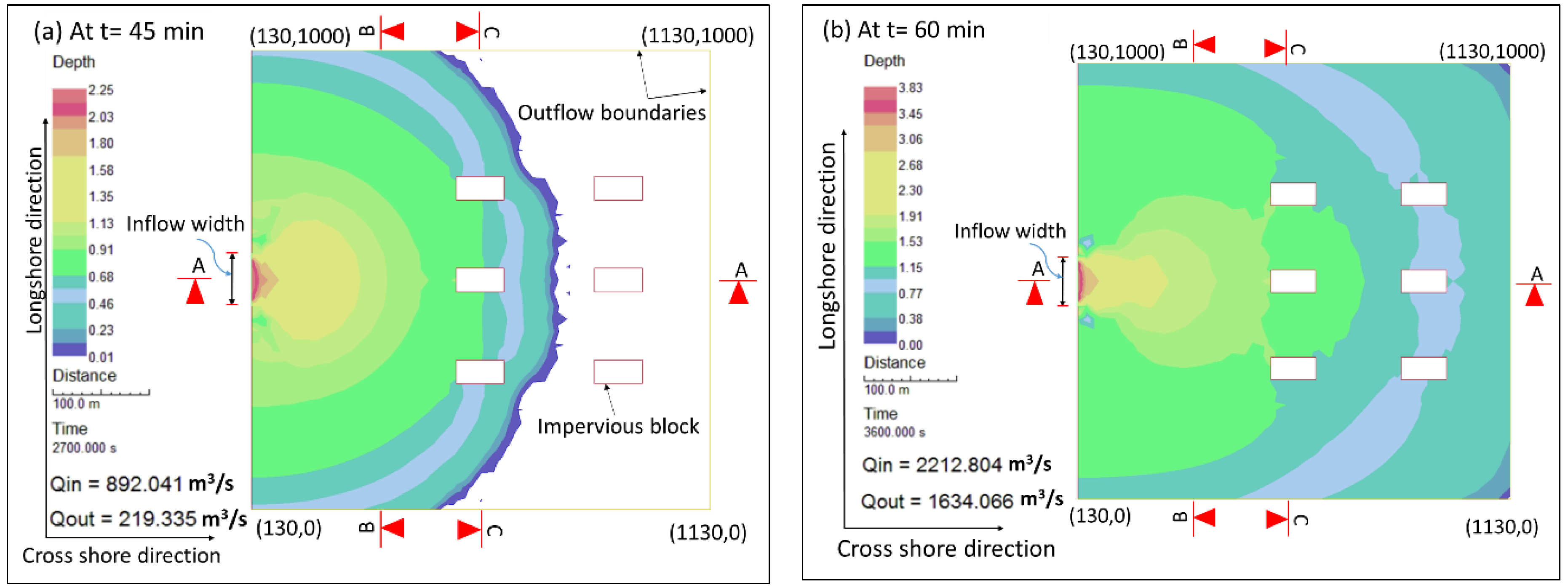
4.2.1. Breach and Flood Propagation Results from XBeach for Load Case LC1

XBeach is applied to simulate both the breaching of the coastal barrier in Figure 3, as well as the induced inundation, considering the rectangular load case LC1 (Figure 2) in addition to the JONSWAP spectrum that represents the offshore wind waves. Figure 12 shows the model set-up in XBeach as well as the induced breaches, inundation and sediment deposition in the form of fans behind the breaches.

The synthetic 2D case in Figure 3 is set-up in XBeach considering the longshore variability of the dune dimensions in addition to defining the buildings as higher ground elevations (Figure 12a). The spatial distribution of the buildings and the locations of the reference points N1, N2 and N3 are shown in Figure 12b. A single breach is developed at almost the lowest point of the crest, resulting in the propagation of seawater in the hinterland as shown in Figure 12c. With the time marching, three other breaches develop around the main breach (Figure 12d). Because of the longshore variability of the dune crest, only one breach was expected to develop at the lowest point of the dune crest, as already observed at the beginning. Indeed, by assuming longshore homogeneity of the strength characteristics of the barrier, this expectation would be justified only for uniformly distributed hydraulic loading alongshore (i.e., with long-crested waves or without any waves). In the case of long-crested waves over a uniformly distributed bathymetry alongshore, one breach might only be expected at the lowest point of the dune crest, since the hydraulic load is uniformly distributed alongshore and, thus, erosion, offshore avalanching and the induced lowering of the dune crest are also uniformly distributed alongshore. In this case, the lowest point of the dune crest would indeed represent the potential location of a unique breach. In the case of short-crested waves (alongshore varying hydraulic loads), which represent the real sea state, the hydraulic load is non-uniformly distributed alongshore (Figure 12e), resulting in wave focusing at local zones in front of the dune. As a result, the erosion, offshore avalanching and the induced lowering of the dune crest may also vary alongshore, which might result in multiple breaches. Because a standard JONSWAP spectrum is used throughout XBeach for wave generation, short-crested waves with an alongshore varying time series of the wave energy are generated, so that erosion and offshore avalanching will also vary alongshore, thus leading to multiple breaches. Consequently, the location of incipient breaching is not only a function of the longshore variability of the dune characteristics, but also depends on the longshore variability of the hydraulic load. Figure 12e shows an example for the variability of the wave height over the model domain at the storm end (t = 1.0 h) and shows that part of the energy is diffracted through the breach induced inlet. In addition, Figure 12f shows that the breaching process results in a significant scour at the location of the main breach as well as in sediment deposition behind the breaches, forming sediment fans.

4.2.2. Water and Sediment Inflow Discharges to the Hinterland

As mentioned in Table 2, the longshore spatial step (dy) is set at 2 m, which means that the 2D model of the considered coastal zone is divided into 500 cross-shore stretches (longshore extend = 1000 m). The total inflow discharge Q(t) over the dune and through the breach induced inlets is obtained by summing all the discharges calculated for each stretch separately at the landward toe of the barrier. Of course, several dune zones are not overtopped, especially those at the lateral edges of the model (Figure 12d), which means that there is no necessity to calculate all the discharges at the landward toe of the barrier for all stretches. However, the inland discharge is calculated for the 500 stretches by following the illustrated approach in Figure 13.

The breaching process results in significant amounts of sediment transported with the water inflow to the hinterland. Therefore, the inland sediment discharge Q_s(t) is also calculated from the outcomes of XBeach using the same approach for calculating the inland water discharge Q(t); i.e., the sediment transport rate over the toe of each individual stretch out of the 500 stretches is calculated separately. As a result, the total inland sediment discharge Q_s(t) through summation of the calculated individual q_s-values is obtained. Figure 14 shows the inland discharge of both water and sediment calculated at the landward toe of the dune.

The significant amounts of saltwater flowing inland, shown in Figure 14, indicate how crucial the breaching process is for the possible contamination of coastal groundwater. For instance, the inland discharge started from zero at the breach initiation phase and increased steadily to reach approximately 2500 $m^3/s$ at the storm end. The water stopped flowing inland after one hour just because the storm is ended. Due to the sudden decrease of the SWL from +5.00 to 0.00 m after 1.0 h, the inland discharge is suddenly decreased; it is counted by negative values, which means that part of the water in the hinterland flows back to the sea after the storm end. The sediment transport rate increases with the flow and stops suddenly with the storm end, which means that the breach would steadily enlarge and deepen as long as the water is flowing inland through the breach. The fluctuations of the sediment hydrograph Q_s(t) in Figure 14 might be explained by the avalanching effect, where the avalanched soil from the lateral sides of the breach represents a pulse-like feeder of sediment. In fact, soil suddenly avalanches in the form of headcut (soil blocks) when the breach side slopes exceed the critical slope for avalanching, resulting in such fluctuations.

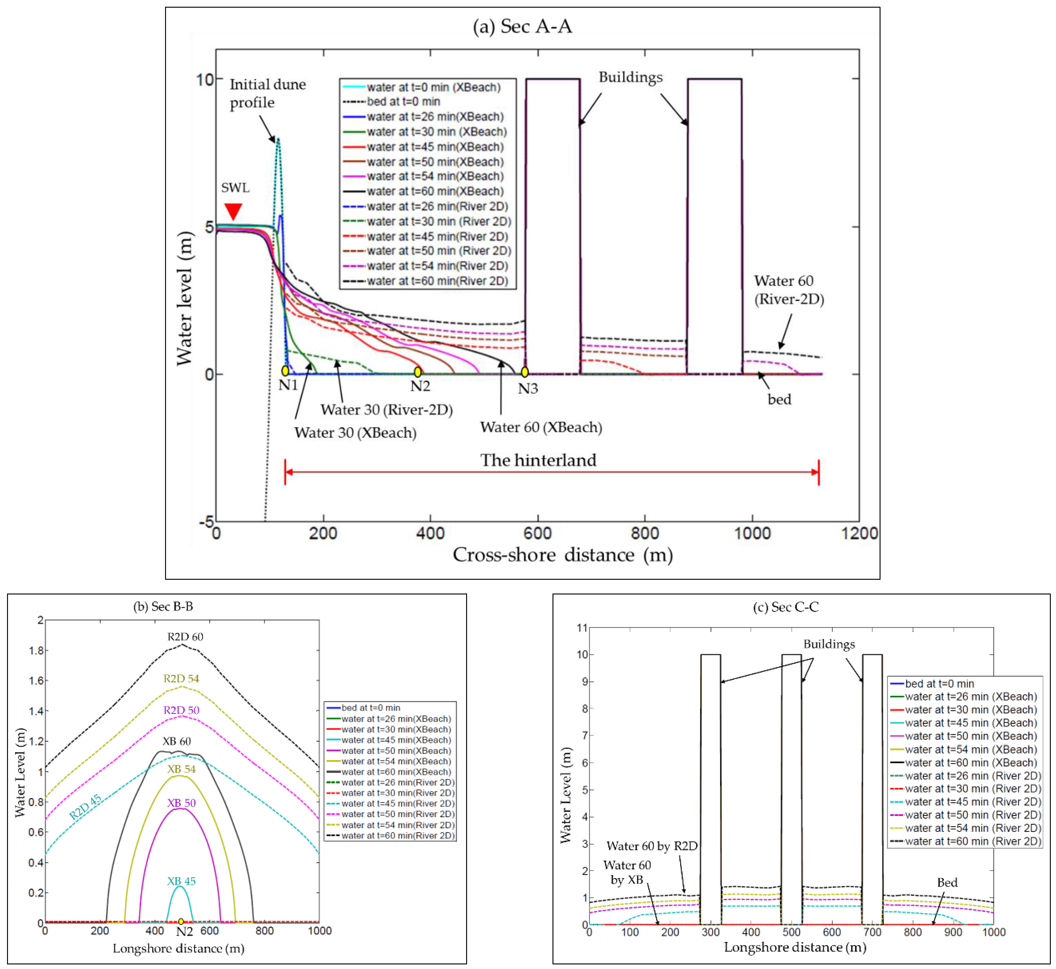
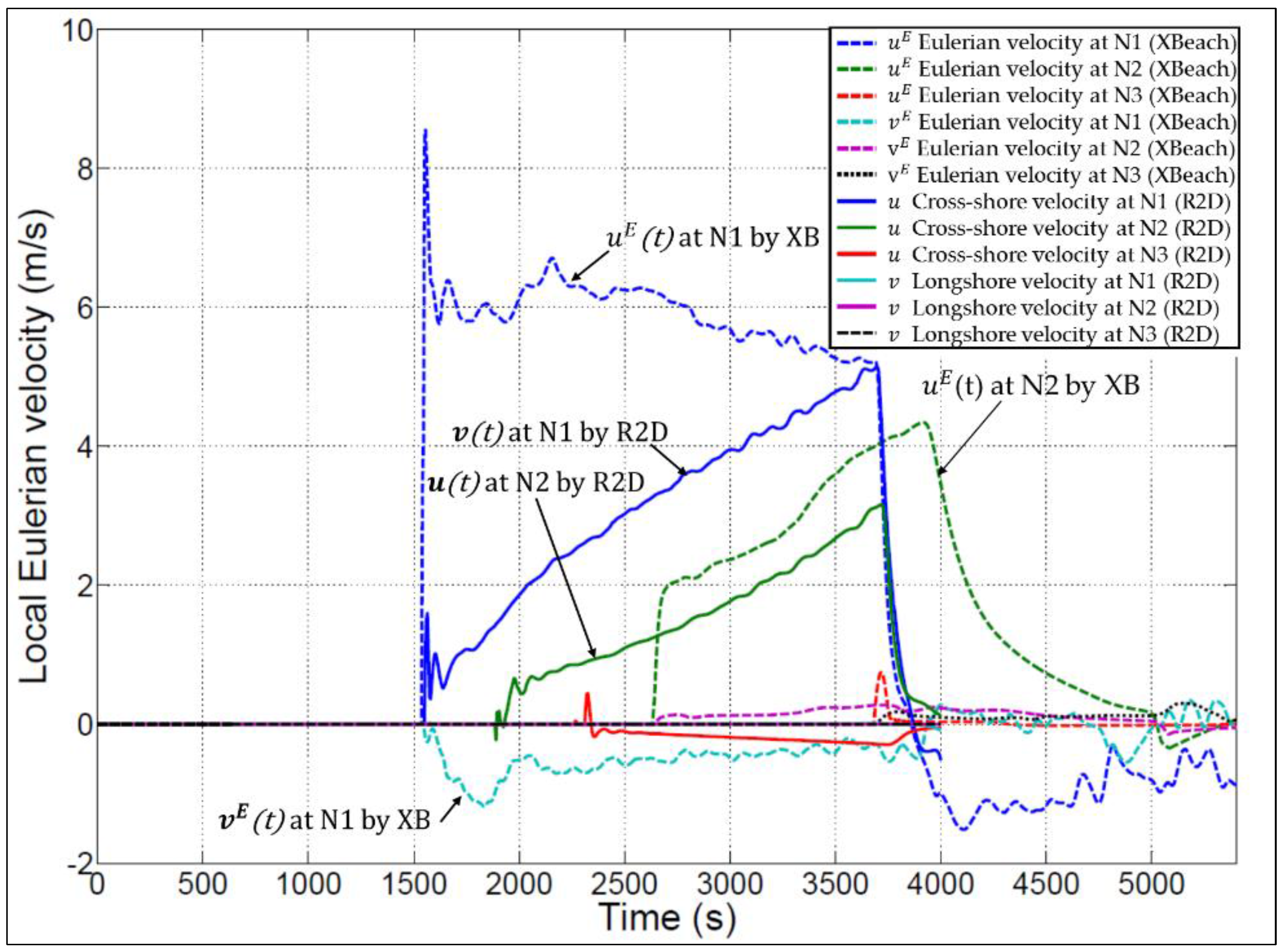
4.2.3. Comparative Analysis of Inundation Modelling Results from XBeach and River-2D

In this 2D case, The River-2D model is used as a benchmarking inundation model to compare the obtained hinterland inundation against the one by XBeach. The same simulation conditions (e.g., bed friction and eddy viscosity) and boundaries are applied in the River-2D model as in XBeach (see Elsayed and Oumeraci, (2016 [66]) for further details). In addition, buildings are defined in the River-2D model as internal no flow boundaries (impervious blocks). Because River-2D calculates the flood propagation without sediment transport, only the inflow water discharge Q(t) from Figure 14 is used as an upstream input to the River-2D model while the sediment inflow discharge Q_s(t) is omitted. In addition, the size of the inflow inlet is fixed at the final size of the four breaches in Figure 12d since the development of the breaches’ dimensions over the simulation time cannot be assigned to River-2D. The flood extent calculated by River-2D at t = 45 min, as well as at the storm end (t = 60 min) are shown in Figure 15a,b, respectively.

Figure 15, in addition, illustrates the water depths in the hinterland, as well as the instantaneous inflow (Q_in) and outflow (Q_out) discharges through the model inlet and through both the lateral and downstream boundaries, respectively. Moreover, Figure 15 visualises the contribution of buildings to the attenuation of the flood propagation in the hinterland. However, when comparing the flood extents, calculated by River-2D in Figure 15a,b, with their counterparts by XBeach in Figure 12 c,d, respectively, a substantial difference in the flood extents and water depths can be noticed. Figure 16 provides comparisons between the temporal evolution of water depths by XBeach and River-2D at Sec A-A, Sec B-B and Sec C-C. The three cross-sections show that the flood extent and water depths by River-2D have higher values as compared to those by XBeach. Such higher values can be attributed to two reasons:

(i)

Assigning the inflow to River-2D through a fixed width (Figure 15) while omitting the evolution of the breach size dimensions as generated by XBeach. Such a fixed inflow width results in wider estimates of the flood extent from the beginning to the end of the simulation.

(ii)

The omission of the momentum conservation principle when passing the inflow hydrograph to River-2D, resulting in subcritical inflow behind the model inlet, which is in contrast to reality.

The higher values for the flood extent and depths by River-2D results in lower values for the flow velocity from River-2D as compared to XBeach. For instance, Figure 17 shows a comparison of the flow velocities at the reference points N1, N2 and N3, revealing lower estimates for the flow velocity from River-2D.

The modelling approaches, using two models separately (overtopping/breaching model for the inflow conditions and CFD model for the subsequent inundation), is not favoured for the following reasons: “manual” transfer of the inflow boundary conditions by considering only mass conservation and omitting momentum conservation, in addition to the non-consideration of the evolution of the inflow width in the common inundation models (see Figure 15). This generally results in higher estimates of the flood extent and depths and sometimes even in non-realistic water levels as shown in Figure 8 and Figure 9, where the water levels at the hinterland inlet exceed the SWL. Therefore, a combined modelling of coastal barrier breaching and induced inundation using XBeach is preferred. For this purpose, a validation of XBeach is performed using the case study of the Het Zwin dam breach.

4.3. Case Study of Het Zwin Dam Breach

The real overflow-induced breaching case of the 1994 artificial dam at Het Zwin (Figure 4) was reproduced in XBeach by Roelvink et al. (2009 [23]). In this study, Roelvink’s breach simulation model is run again considering the model settings in Table 3. The measured SWL at the measuring station MS2 (Figure 4b) is assigned to the model as the seaward hydraulic load, and no wave action is considered. The dam breach results are presented in Section 4.3.1, while Section 4.3.2 presents a comparison of the observed and modelled water depths and flow velocities at the measuring stations in Figure 4b. Section 4.3.3 provides the calculations of the inland discharge as well as a comparison of the total inland volume and the mean tidal prism at Het Zwin.

4.3.1. Reproduction of the Zwin Dam Breach by XBeach

The dam breach at Het Zwin is a field breaching test induced by overflow; i.e., the breach development is only induced by a landward erosion of the dam. Figure 18a,b present the breach development in cross-shore and longshore directions, respectively. Moreover, Figure 18c presents a comparison of the observed and simulated breach widths. Due to the overflow, the landward side of the dam erodes, causing a crest lowering at the breach location as well as an avalanching of the lateral sides of the breach. With the time marching, the dam body at the breach location is totally overwashed. The overwash phase is followed by scouring at the breach location and sediment deposition behind the dam (Figure 18a). The avalanching algorithm in XBeach enables simulating the lateral development of the breach induced channel (Figure 18b). The breach process extent until filling the tidal prism (i.e., until the water levels in front and behind the dam become equal). The high correlation ($R^2$), as well as the relatively low Root Mean Square Error (RMSE) between the observed and simulated breach widths, demonstrates the capability of XBeach as a breaching model ($R^2=0.98$ and RMSE = 2.73 m). A comparison of these statistical indicators with those calculated by Roelvink et al. (2009 [23]) is presented in Elsayed and Oumeraci, (2016 [39]).

4.3.2. Observed vs Modelled Water Depths and Flow Velocities at Het Zwin Breach

The comparison of the observed and simulated water depths and flow velocities at different points, indicated in Figure 4b, are shown in Figure 19. At t = 0 (time of pilot channel enforcement), about 10 min prior to maximum water level, the water level at the seaside was 2.72 m + NAP (see observed water level at MS2). At t = 10 min, a water level of 2.75 m + NAP is reached. For the remainder of the test, which has a total duration of 1.0 h, the water level decreases to 2.4 m + NAP. After 1.0 h, the water level behind the breach equals the sea level and the breach stops growing. Because of the water flow in the landside, the water level at MS4 and MS5 increases dramatically until reaching the sea level and the flow velocity at these points increases until reaching the peak velocity after 20 min, then both decrease due to the breaching process becoming increasingly slower until it stops.

The comparison between the observed and simulated flow velocities and water depths in Figure 19 illustrates the relatively good prediction capability of XBeach. The peak flow velocities at MS4 and MS5 are overestimated by 6% to 15%, while it is underestimation by ca. 30% at station MS3. The latter deviations from the observed values could be attributed to the difference between the observed and simulated breach dimensions. In fact, this may be explained by the calculated narrower breach width at the start of the breach as shown in Figure 18c, which results in a higher flow velocity through the breach and thus at the measuring stations MS4 and MS5. This justification is confirmed by the fact that the narrower breach width will allow less inland flow rates and therefore less simulated versus observed flow velocity at MS3. Nevertheless, these overall comparisons in Figure 19 still demonstrate the capability of XBeach to properly calculate the flow velocity and water depth at any local point in the hinterland. For future improvements, the prediction capability of the breach dimensions will definitely lead to a better prediction of the flow velocity and water depth in the hinterland.

4.3.3. Water Discharge through the Dam Breach

The 2DH model of the Zwin dam was discretized into 101 cross-shore stretches in the longshore direction (e.g., Figure 13). These stretches have variable widths that vary from 0.5 m at the breach location to approximately 50 m far away from the breach (see, e.g., Elsayed and Oumeraci, 2016 [66]). In order to calculate the total inland discharge through the breach-induced channel, the inland discharge should be calculated over the 101 cross-shore stretches using the same schematic approach as in Figure 13. As a result, the water inflow discharge $q_i$ is calculated for each of the 101 cross-shore stretches in Figure 20a, which shows that the dam was overtopped at only five cross-shore stretches at the beginning of the simulation. With the time marching, many other stretches are also overtopped due to the breach growth. The summation of the inflow discharges $q_i$ in Figure 20a provides the total inflow hydrograph Q(t) as shown in Figure 20b. Q(t) is zero at t = 0 (time of pilot channel enforcement) and increases to 161 $m^3/s$ after 40 min and reduces again to zero because the water levels at the upstream and downstream dam sides become equal. The area under the water discharge curve in Figure 20b represents the total volume of the inflow water (total volume = 308,430 $m^3$). Such volume depends on the polder area of the tidal inlet as well as on the sea water level; i.e., with higher sea water levels, higher inflow volumes are expected. The latter volume is near to the value of the mean tidal prism (350,000 $m^3$), thus indicating the XBeach capability to predict the flood extent properly. The difference between the total inland volume (308430 $m^3$) and the mean tidal prism (350,000 $m^3$) can be attributed to the difference of the mean tidal level (2.85 m + NAP) to level 2.40 m + NAP at the end of the breaching process (see Figure 19a). Such a decrease in the sea water level decreases the capacity of the tidal inlet.

The comparison between the observed and the calculated (i) breach widths in Figure 18c and (ii) water depths and flow velocities (Figure 19) as well as the comparison between the volume of the tidal prism and the calculated total inland discharge demonstrate the capability of XBeach to properly calculate the breach development together with the resulting water depths, flow velocities and flood extent in the hinterland. These results, therefore, support the suitability of applying XBeach for the combined modelling of barrier breaching and the subsequent flood.

5. Discussion of the Results

The comparative analyses of

(i)

the results from the current modelling approach, applying separately an overtopping/breaching model to calculate the inflow hydrograph Q(t) and a common inundation NLSWEs-based model, such as HEC-RAS and River-2D, using Q(t) as an inflow boundary condition at the barrier to simulate the flood propagation in the hinterland, and

(ii)

the results of XBeach applied to simulate, together, both breaching and subsequent inundation, have clearly demonstrated the advantages of the latter modelling approach. In fact, among the available open-source hydro-morphodynamic models, XBeach is the most appropriate tool for the latter approach.

Indeed, in addition to solving numerically the same governing equations (NLSWEs) as the other common inundation models, XBeach has the following capabilities and advantages:

(i)

XBeach can generate real sea conditions through generating alongshore varying time series of wave energy (alongshore varying hydraulic loads), where the effect of waves is introduced as a source term in the NLSWEs;

(ii)

the CFD module can simulate wave overtopping and overflow processes in combination, the flow through the developing breach and the subsequent coastal inundation processes in a single simulation;

(iii)

the morphodynamic module can properly calculate sediment transport and the resulting morphological changes and also includes a soil avalanching algorithm making Xbeach capable of to properly simulating the evolution of barrier breaching.

The comparative analysis of the water depths, velocities and flood extent in the hinterland, due to barrier breaching as obtained from XBeach and those obtained by the two benchmarking inundation models (HEC-RAS and River-2D), has revealed the following weaknesses of the uncoupled modelling of breaching and subsequent inundation:

(i)

The use of hydrograph Q(t) as inflow conditions to the common inundation models is in line with the mass conservation principle, but the flow velocity v(t) which cannot be accounted for in the inflow conditions is also crucial as it provides, together with Q(t) the momentum;

(ii)

Higher estimates for the flood extent and water depths, mainly due to the omission of the momentum conservation when transferring the flow from the breaching model to the inundation model (in some cases this may even lead to physically wrong water levels as shown in Figure 8 and Figure 9);

(iii)

No account of the evolution of the inflow width (see Figure 15) in the common inundation models.

In this study, these weaknesses are overcome by the combined modelling of breaching and subsequent inundation using XBeach, as demonstrated by the afore-described results of the dam breach case in Het Zwin. Moreover, this study has addressed barrier breaching under diverse hydraulic loads. The hydraulic forcing from the sea constitutes the main driver for coastal erosion, coastal barrier breaching and subsequent flooding. The loading from the sea may be subdivided into two main load categories (a) sea level changes due to storm surges, external surges, seiches, wave set-up, astronomical tides and further long waves of different origins, and (b) storm-induced (short) waves. The former load category represents, in essence, very long waves that generally induce a set-up of the sea level so that the shorter storm waves riding on a higher mean sea level will hit, overtop and/or overflow the natural and man-made barriers of the sea defence system, possibly causing coastal erosion and barrier breaching. Therefore, with the higher sea level, due to the first load category alone (i.e., without storm-induced waves), barrier breaching is unlikely as long as the sea level is less than the lowest crest level of the barrier. As soon as the lowest crest is exceeded, incipient overflow occurs, possibly resulting in a landward erosion and breaching of the barrier. When the storm-induced waves directly impact the dune face exposed to the sea, the latter erodes under repeated wave impacts, wave run-up and run-down. Besides the sediment transported offshore by wave run-down, a seaward dune avalanching would result, which lowers the dune crest, making it vulnerable by the subsequent wave run-up events. As a result, the waves may overtop the barrier causing erosion of the landward side and possibly lowering the crest. In addition to wave overtopping, overflow above the lowered dune crest may then occur, leading to higher flow velocities that reinforce the landward erosion.

The study has demonstrated that dune breach initiation is not only a function of the longshore variability of the dune topography (e.g., crest level), but also a function of the longitudinal variability of the hydraulic load as a result of wave transformation due to the longshore variability of the foreshore morphology mutually interacting with the waves (see Figure 12). This might explain why many breaches developed where they were not expected. By adding the residual resistance of the dune material (Elsayed and Oumeraci, 2016 [39]; Morris, 2011 [67]) to these triggering factors of breach initiation, the prediction of the breaching process becomes much more complex. In fact, the longshore variability of the resistance of the dune material may be caused by the presence of weak spots (e.g., bioturbation) or zones of less interlocked sediments and less consolidated soils (Figure 21).

Dune breach initiation is, therefore, a function of (a) the longshore variability of the dune topography (e.g., crest level), (b) the longitudinal variability of the hydraulic load (e.g., wave focusing) and (c) the longshore variability of the residual resistance of the dune (e.g., weak spots due to bioturbation or low soil consolidation). The latter two triggering factors are highly uncertain and thus decrease the predictability of the potential locations of breaches. Figure 22 illustrates how these triggering factors affect breach initiation. Moreover, it also highlights that the highest uncertainties are expected for the case where the hydraulic load, the topography and the resistance of the dune all together, vary alongshore. In fact, XBeach does not yet account for the spatial variability of the residual resistance of dunes, so it might represent a candidate topic for further development of XBeach.

The study has also briefly addressed the effect of large roughnesses (i.e., large obstacles such as buildings) on the attenuation of flood propagation in the hinterland. For this purpose, two possibilities might be considered in the inundation modelling with XBeach: setting very high roughness values or defining higher ground elevations at the obstacle locations. In this study, the latter option is applied in XBeach; the higher ground elevations at the obstacle locations are specified to be hard and impermeable in order to avoid any erosion and/or avalanching. However, in the River-2D model, the buildings are treated as impervious internal boundaries. Such internal boundaries facilitate the treatment of complex building geometries. XBeach uses a structured grid form of quadrilateral cells, which might be inflexible enough to represent complex building geometries. For further development of XBeach, it is suggested to examine an unstructured grid option in order to avoid very fine grids.

6. Conclusions and Remarks

This study aimed at applying the hydro-morphodynamic model XBeach as an inundation model and a breaching model in combination, rather than using two uncoupled models to simulate a coastal barrier breaching and the induced flooding. The results of this study have demonstrated a new promising application of XBeach and its potential for modelling, together, both dune breaching and subsequent flood propagation in coastal zones. As a CFD model using a NLSWEs solver coupled with a morphodynamic model, which includes a soil avalanching module, XBeach has the capability to integrally simulate coastal inundation induced by extreme storm surges with the advantage of reproducing the mutual interaction between hydrodynamics (e.g., flow in the breach channel) and morphodynamics, including soil avalanching (e.g., breach development). An attempt has been made to demonstrate the advantage of this combined modelling approach using a single hydro-morphodynamic model (XBeach) instead of the current approach using two uncoupled models. In fact, the proposed modelling approach (XBeach) showed a good agreement between the flow velocities and water depths observed in the real case study of the Het Zwin (sand) dam breach. In contrast, the flood extent and flow depths predicted by the current approaches are up to 40% larger than the observed values.

The effect of alongshore variability of both hydraulic loads and barriers topography on the location of breach initiation has been preliminarily implemented in the simulations of this study. Moreover, the longshore variability of resistance characteristics of coastal barriers’ materials (e.g., distribution of material inhomogeneity and of weak points along the barrier) on the location of breach initiation has also been briefly discussed. Though the latter was not implemented in the proposed model, it will remain, besides the longshore variability of the hydraulic loads, one of the biggest research challenges.

References

1. Smith, K. Environmental Hazards: Assessing Risk and Reducing Disaster, 6th ed.; Routledge: London, UK, 2013. [Google Scholar]
2. Xu, L.; He, Y.; Huang, W. A multi-dimensional integrated approach to assess flood risks on a coastal city, induced by sea-level rise and storm tides. Environ. Res. Lett. 2016, 11, 014001. [Google Scholar]
3. Kraus, N.C.; Wamsley, T.V. Coastal Barrier Breaching. Part 1. Overview of Breaching Processes. DTIC Document. 2003. Available online: http://oai.dtic.mil/oai/oai?verb=getRecord&metadataPrefix=html&identifier=ADA588872 (accessed on 5 December 2015).
4. Roger, S.; Dewals, B.; Schuettrumpf, H.; Erpicum, S.; Archambeau, P.; Pirotton, M.; Schwanenberg, D.; Dewals, B. Hybrid modelling of dike-break induced flows. In River Flow 2010, Proceedings of the International Conference on Fluvial Hydraulics, Braunschweig, Germany, 8–10 September 2010; Dittrich, A., Koll, K., Aberle, J., Geisenhainer, P., Eds.; Karlsruhe: Bundesanstalt für Wasserbau, 2010; pp. 523–531. [Google Scholar]
5. Bisschop, F.; Visser, P.; van Rhee, C.; Verhagen, H.J. Erosion due to high flow velocities: A description of relevant processes. In Proceedings of 32nd Conference on Coastal Engineering, Shanghai, China, 30 June–5 July 2010; Lynett, P., Ed.; International Conference on Coastal Engineering (ICCE), 2010; Volume 1, p. 24. [Google Scholar]
6. Wu, W.; Altinakar, M.S.; Song, C.R.; Al-Riffai, M.; Bergman, N.; Bradford, S.F.; Cao, Z.; Chen, Q.J.; Constantinescu, S.G.; Duan, J.G. Earthen embankment breaching. J. Hydraul. Eng. 2011, 137, 1549–1564. [Google Scholar]
7. Sills, G.; Vroman, N.; Wahl, R.; Schwanz, N. Overview of New Orleans levee failures: Lessons learned and their impact on national levee design and assessment. J. Geotech. Geoenviron. Eng. 2008, 134, 556–565. [Google Scholar] [CrossRef]
8. Yang, J.; Graf, T.; Herold, M.; Ptak, T. Modelling the effects of tides and storm surges on coastal aquifers using a coupled surface-subsurface approach. J. Contam. Hydrol. 2013, 149, 61–75. [Google Scholar] [CrossRef] [PubMed]
9. Yang, J.; Graf, T.; Ptak, I.T. Sea level rise and storm surge effects in a coastal heterogeneous aquifer: A 2d modelling study in northern Germany. Grundwasser Z. Fachsekt. Hydrogeol. 2015, 20, 39–51. [Google Scholar] [CrossRef]
10. Christensen, B.B.; Drønen, N.; Klagenberg, P.; Jensen, J.; Deigaard, R.; Sørensen, P. Multiscale modelling of coastal flooding. In Proceedings of 7th International Conference for Coastal Dynamics, Arcachon Convention Centre, Arcachon, France, 24–28 June 2013; Jörg-Olaf, W., Ed.; Springer, 2013; pp. 339–350. [Google Scholar]
11. He, Z.; Hu, P.; Zhao, L.; Wu, G.; Pähtz, T. Modeling of breaching due to overtopping flow and waves based on coupled flow and sediment transport. Water 2015, 7, 4283–4304. [Google Scholar] [CrossRef]
12. Hinkel, J.; Lincke, D.; Vafeidis, A.T.; Perrette, M.; Nicholls, R.J.; Tol, R.S.; Marzeion, B.; Fettweis, X.; Ionescu, C.; Levermann, A. Coastal flood damage and adaptation costs under 21st century sea-level rise. Proc. Natl. Acad. Sci. USA 2014, 111, 3292–3297. [Google Scholar] [CrossRef] [PubMed]
13. Cheung, K.; Phadke, A.; Wei, Y.; Rojas, R.; Douyere, Y.-M.; Martino, C.; Houston, S.; Liu, P.-F.; Lynett, P.; Dodd, N. Modelling of storm-induced coastal flooding for emergency management. Ocean Eng. 2003, 30, 1353–1386. [Google Scholar] [CrossRef]
14. Bates, P.D.; Dawson, R.J.; Hall, J.W.; Horritt, M.S.; Nicholls, R.J.; Wicks, J.; Hassan, M.A.A.M. Simplified two-dimensional numerical modelling of coastal flooding and example applications. Coast. Eng. 2005, 52, 793–810. [Google Scholar] [CrossRef]
15. Chini, N.; Stansby, P.; Rogers, B.; Vacondio, R.; Mignosa, P. State-of-the-art coastal inundation models applied to the 2007 Norfolk storm. In Comprehensive Flood Risk Management: Research for Policy and Practice. Proceedings of the 2nd European Conference on Flood Risk Management FLOODrisk2012, Rotterdam, The Netherlands, 20–22 November 2012; Klijn, F., Schweckendiek, T., Eds.; CRC Press/Balkema: London, UK, 2012; p. 8. [Google Scholar]
16. Smith, R.A.; Bates, P.D.; Hayes, C. Evaluation of a coastal flood inundation model using hard and soft data. Environ. Model. Softw. 2012, 30, 35–46. [Google Scholar] [CrossRef]
17. McCabe, M.; Stansby, P.; Apsley, D. Random wave runup and overtopping a steep sea wall: Shallow-water and Boussinesq modelling with generalised breaking and wall impact algorithms validated against laboratory and field measurements. Coast. Eng. 2013, 74, 33–49. [Google Scholar] [CrossRef]
18. Chini, N.; Stansby, P. Extreme values of coastal wave overtopping accounting for climate change and sea level rise. Coast. Eng. 2012, 65, 27–37. [Google Scholar] [CrossRef]
19. Gallien, T.; Sanders, B.; Flick, R. Urban coastal flood prediction: Integrating wave overtopping, flood defenses and drainage. Coast. Eng. 2014, 91, 18–28. [Google Scholar] [CrossRef]
20. Tsoukala, V.K.; Chondros, M.; Kapelonis, Z.G.; Martzikos, N.; Lykou, A.; Belibassakis, K.; Makropoulos, C. An integrated wave modelling framework for extreme and rare events for climate change in coastal areas–the case of Rethymno, Crete. Oceanologia 2016, 58, 71–89. [Google Scholar] [CrossRef]
21. Pullen, T.; Allsop, N.; Bruce, T.; Kortenhaus, A.; Schuttrumpf, H.; van der Meer, J. EurOtop (European overtopping manual): Wave overtopping of sea defences and related structures: Assessment manual. Available online: Http://www.Overtopping-manual.Com/manual.Html (accessed on 20 May 2016).
22. Vousdoukas, M.I.; Voukouvalas, E.; Annunziato, A.; Giardino, A.; Feyen, L. Projections of extreme storm surge levels along Europe. Clim. Dynam. 2016. [Google Scholar] [CrossRef]
23. Roelvink, D.; Reniers, A.; van Dongeren, A.; de Vries, J.V.T.; McCall, R.; Lescinski, J. Modelling storm impacts on beaches, dunes and barrier islands. Coast. Eng. 2009, 56, 1133–1152. [Google Scholar] [CrossRef]
24. Giardino, A.; Briére, C.; Deserti, M.; Malmonado, V.M.; Reggiani, P.; van Ormondt, M.; Valentini, A.; van der Werf, J. Operational modelling applications for coastal engineering: New developments. In MEDCOAST 2011. Proceedings of the 10th International Conference on the Mediterranean Coastal Environment, Rhodes, Greece, 25–29 October 2011; Özhan, E., Ed.; Mediterranean Coastal Foundation, 2011. [Google Scholar]
25. Barnard, P.L.; van Ormondt, M.; Erikson, L.H.; Eshleman, J.; Hapke, C.; Ruggiero, P.; Adams, P.N.; Foxgrover, A.C. Development of the coastal storm modelling system (COSMOS) for predicting the impact of storms on high-energy, active-margin coasts. Nat. Hazards 2014, 74, 1095–1125. [Google Scholar] [CrossRef]
26. Gallien, T.; Guza, R. Modelling and observations of wave overtopping flooding on a southern California beach. In Proceedings of the 36th IAHR World Congress, The Hague, The Netherlands, 28 June–3 July 2015; International Association for Hydro-Environment Engineering and Research-IAHR: Madrid, Spain, 2015; p. 2. [Google Scholar]
27. Gallien, T. Validated coastal flood modelling at Imperial Beach, California: Comparing total water level, empirical and numerical overtopping methodologies. Coast. Eng. 2016, 111, 95–104. [Google Scholar] [CrossRef]
28. Palmsten, M.L.; Splinter, K.D. Observations and simulations of wave runup during a laboratory dune erosion experiment. Coast. Eng. 2016, 115, 58–66. [Google Scholar] [CrossRef]
29. Wadey, M.P.; Nicholls, R.J.; Hutton, C. Coastal flooding in the Solent: An integrated analysis of defences and inundation. Water 2012, 4, 430–459. [Google Scholar] [CrossRef]
30. Worni, R.; Huggel, C.; Clague, J.J.; Schaub, Y.; Stoffel, M. Coupling glacial lake impact, dam breach, and flood processes: A modeling perspective. Geomorphology 2014, 224, 161–176. [Google Scholar] [CrossRef]
31. Elsayed, S.M. Comparative study of different scenarios for the morphological evolution in a river stream. Master’s Thesis, Politecnico di Milano, Milan, Italy, 2013. [Google Scholar]
32. Radice, A.; Elsayed, S.M. Hydro-Morphologic Modelling for Different Calamitous Scenarios in a Mountain Stream. In Proceedings of the River Flow 2014: 7th International Conference on Fluvial Hydraulics, Lausanne, Switzerland, 3–5 September 2014; Schleiss, A.J., de Cesare, G., Franca, M.J., Pfister, M., Eds.; CRC Press/Balkema: Leiden, The Netherlands, 2014. [Google Scholar]
33. Fan, X.; Tang, C.; van Westen, C.; Alkema, D. Simulating dam-breach flood scenarios of the Tangjiashan Landslide dam-induced by the Wenchuan Earthquake. Nat. Hazards Earth Syst. Sci. 2012, 12, 3031–3044. [Google Scholar] [CrossRef]
34. Popescu, I.; Jonoski, A.; van Andel, S.; Onyari, E.; Moya Quiroga, V. Integrated modelling for flood risk mitigation in Romania: Case study of the Timis–Bega river basin. Int. J. River Basin Manag. 2010, 8, 269–280. [Google Scholar] [CrossRef]
35. Tadesse, Y.B.; Fröhle, P. An integrated approach to simulate flooding due to river dike breach. In Proceedings of 11th International Conference on Hydroinformatics (HIC 2014), New York, NY, USA, 17–21 August 2014; CUNY Academic Works, 2014. [Google Scholar]
36. Bertin, X.; Li, K.; Roland, A.; Zhang, Y.J.; Breilh, J.F.; Chaumillon, E. A modelling based analysis of the flooding associated with Xynthia, Central Bay of Biscay. Coast. Eng. 2014, 94, 80–89. [Google Scholar] [CrossRef]
37. Roland, A.; Zhang, Y.J.; Wang, H.V.; Meng, Y.; Teng, Y.C.; Maderich, V.; Brovchenko, I.; Dutour-Sikiric, M.; Zanke, U. A fully coupled 3D wave-current interaction model on unstructured grids. J. Geophys. Res. Oceans 2012. [Google Scholar] [CrossRef]
38. Vousdoukas, M.I.; Voukouvalas, E.; Mentaschi, L.; Dottori, F.; Giardino, A.; Bouziotas, D.; Bianchi, A.; Salamon, P.; Feyen, L. Developments in large-scale coastal flood hazard mapping. Nat. Hazards Earth Syst. Sci. 2016, 16, 1841–1853. [Google Scholar] [CrossRef]
39. Elsayed, S.M.; Oumeraci, H. Effect of beach slope and grain-stabilization on coastal sediment transport: An attempt to overcome the erosion overestimation by XBeach. Coast. Eng. 2016. submitted for publication. [Google Scholar]
40. Bendoni, M. Salt Marsh Edge Erosion due to Wind-Induced Waves. Ph.D. Thesis, Technische Universität Braunschweig & University of Florence, Braunschweig, Germany, 2015. [Google Scholar]
41. De Vet, P. Modelling Sediment Transport and Morphology during Overwash and Breaching Events. Master’s Thesis, Delft University of Technology, Delft, The Netherlands, 2014. [Google Scholar]
42. Hartanto, I.M.; Beevers, L.; Popescu, I.; Wright, N.G. Application of a coastal modelling code in fluvial environments. Environ. Model. Softw. 2011, 26, 1685–1695. [Google Scholar] [CrossRef]
43. Beevers, L.; Popescu, I.; Pan, Q.; Pender, D. Applicability of a coastal morphodynamic model for fluvial environments. Environ. Model. Softw. 2016, 80, 83–99. [Google Scholar] [CrossRef]
44. Vreugdenhil, C.B. Numerical Methods for Shallow-Water Flow; Springer Science & Business Media: Dordrecht, The Netherlands, 2013; Volume 13. [Google Scholar]
45. Weiyan, T. Shallow Water Hydrodynamics: Mathematical Theory and Numerical Solution for a Two-Dimensional System of Shallow-Water Equations; Water&Power Press and Elsevier Science Publishers: Beijing, China, 1992; Volume 55. [Google Scholar]
46. Saint-Venant, A.D. Theorie du mouvement non permanent des eaux, avec application aux crues des rivieres et a l’introduction de marees dans leurs lits. Comptes rendus des seances de l’Academie des Sciences 1871, 36, 174–154. [Google Scholar]
47. Steffler, P.; Blackburn, J. River 2D Two-Dimensional Depth-Averaged Model of River Hydrodynamics and Fish Habitat: Introduction to Depth Averaged Modelling and User’s; University of Alberta. Available online: http://www.river2d.ualberta.ca/ (accessed on 2 March 2016).
48. Szymkiewicz, R. Numerical stability of implicit four-point scheme applied to inverse linear flow routing. J. Hydrol. 1996, 176, 13–23. [Google Scholar] [CrossRef]
49. Meyer-Peter, E.; Müller, R. Formulas for Bed-Load Transport: Report on Second Meeting of International Association for Hydraulics Research (IAHR); IAHR: Stockholm, Sweden, 1948. [Google Scholar]
50. Pender, D.; Patidar, S.; Haynes, H. Incorporating river bed level changes into flood risk modelling. In Proceedings of the 36th IAHR World Congress, The Hague, The Netherlands, 28 June–3 July 2015; Tailor & Francis Groop: The Hague, The Netherlands, 2015. [Google Scholar]
51. Brunner, G.W. HEC-RAS River Analysis System. Hydraulic Reference Manual. Version 5.0; United States Army Corps of Engineers: Davis, CA, USA, 2016. [Google Scholar]
52. Roelvink, D.; van Dongeren, A.; McCall, R.; Hoonhout, B.; van Rooijen, A.; van Geer, P.; de Vet, P.; Nederhoff, K.; Quataert, E. XBeach Technical Reference: Kingsday Release (Technical Report: Model Description and Reference Guide to Functionalities); Deltares, UNESCO-IHE Institute of Water Education and Delft University of Technology: Delft, The Netherlands, 2015; p. 141. [Google Scholar]
53. Holthuijsen, L.; Booij, N.; Herbers, T. A prediction model for stationary, short-crested waves in shallow water with ambient currents. Coast. Eng. 1989, 13, 23–54. [Google Scholar] [CrossRef]
54. Buckley, M.; Lowe, R.; Hansen, J. Evaluation of nearshore wave models in steep reef environments. Ocean Dyn. 2014, 64, 847–862. [Google Scholar] [CrossRef]
55. Sultan, N.J. Irregular Wave-Induced Velocities in Shallow Water; Ocean Engineering Department Texas A&M University: College Station, Texas, USA, 1992. [Google Scholar]
56. Vetsch, D.; Müller, R.; Rousselot, P.; Volz, C.; Vonwiller, L.; Farshi, D.; Veprek, R.; Fäh, R. Basement Reference Manual; the Laboratory of Hydraulics, Hydrology and Glaciology (VAW) of the Swiss Federal Institute of Technology (ETH): Zurich, Switzerland, 2016; Available online: http://www.basement.ethz.ch/ (accessed on 30 May 2016).
57. Andrews, D.G.; McIntyre, M. An exact theory of nonlinear waves on a lagrangian-mean flow. J. Fluid Mech. 1978, 89, 609–646. [Google Scholar] [CrossRef]
58. Walstra, D.; Roelvink, D.; Groeneweg, J. Calculation of wave-driven currents in a 3d mean flow model. In Proceedings of the 27th International Conference on Coastal Engineering ICCE, Sydney, Australia, 16–21 July 2000; Edge, B.L., Ed.; ASCE, 2001; Volume 2, pp. 1050–1063. [Google Scholar]
59. Ambrosio, B.; Siegle, E. Wave energy levels at inlet channel margins: The effects of the ebb-tidal delta morphology. In Proceedings of the 17th Physics of Estuaries and Coastal Seas (PECS) Conference, Porto de Galinhas, Pernambuco, Brazil, 19–23 October 2014; FCERM.net: Pernambuco, Brazil, 2014; p. 4. [Google Scholar]
60. Swartenbroekx, C.; Soares-Frazão, S.; Staquet, R.; Zech, Y. Two-dimensional operator for bank failures induced by water-level rise in dam-break flows. J. Hydraul. Res. 2010, 48, 302–314. [Google Scholar] [CrossRef]
61. Evangelista, S.; Greco, M.; Iervolino, M.; Leopardi, A.; Vacca, A. A new algorithm for bank-failure mechanisms in 2d morphodynamic models with unstructured grids. Int. J. Sediment Res. 2015, 30, 382–391. [Google Scholar] [CrossRef]
62. Wainwright, D.; Baldock, T. Measurement and modelling of an artificial coastal lagoon breach. Coast. Eng. 2015, 101, 1–16. [Google Scholar] [CrossRef]
63. Vellinga, P. Beach and Dune Erosion During Storm Surges. Ph.D. Thesis, Delft University of Technology, Delft, The Netherlands, 1986. [Google Scholar]
64. Visser, P. Breach Growth in Sand-Dikes. Ph.D. Thesis, Delft University of Technology, Delft, The Netherlands, 1998. [Google Scholar]
65. Bakker, W.; van der Graaff, J.; Kraak, A.; Smit, M.; Snip, D.; Steetzel, H.; Visser, P. Het Zwin, Successen en Lessen: Bresgroeiexperimenten 6 en 7 Oktober 1994 “Het Totale Experiment Geslaagd”; TU Delft, Department Hydraulic Engineering: Delft, The Netherlands, 1996. [Google Scholar]
66. Elsayed, S.M.; Oumeraci, H. Breaching of Coastal Barriers Under Extreme Storm Surges and Implications for Groundwater Contamination: Application of XBeach in Coastal Flood Propagation; TU Braunschweig: Internal report; Leichtweiß-Institut für Wasserbau: Braunschweig, Germany, 2016. [Google Scholar]
67. Morris, M.W. Breaching of Earth Embankments and Dams. Ph.D. Thesis, Open University, UK, 2011. [Google Scholar]
Figure 1. Test case 1: 1D synthetic cross-shore profile (a) 1D synthetic profile used in XBeach to simulate a 1D overwash event and the induced flood propagation in the hinterland and (b) the inland discharge Q(t) is computed from XBeach at point P2, where Q(t) serves as the inflow boundary condition for the HEC-RAS inundation model for the hinterland. The outcomes of the inundation from XBeach and HEC-RAS are compared at reference points P3, P4 and P5.
Hydrology 03 00032 g001
Figure 2. Synthetic cases of the sea water level (SWL) rise under the effects of both meteorological and astronomical tides during the simulation interval (1.0 h).
Hydrology 03 00032 g002
Figure 3. Test case 2: Synthetic 2DH case study shows the sea, the dune, and the hinterland, including the building locations in the hinterland, Sec A-A (cross-shore cross-section), Sec B-B and Sec C-C (alongshore sections) show the important details.
Hydrology 03 00032 g003
Figure 4. Test case 3: The 1994 dam at Het Zwin: (a) dimensions of the dam and the enforced pilot channel (Sec X-X), (b) locations of the measuring stations, after Visser (1998 [64]).
Hydrology 03 00032 g004
Figure 5. Evolution of the bed level (BL) and water level (WL) for the synthetic profile in Figure 1a under load case LC1 as defined in Figure 2.
Hydrology 03 00032 g005
Figure 6. Evolution of the bed level (BL) and water level (WL) for the synthetic profile in Figure 1a under load case 2 (LC2) as defined in Figure 2.
Hydrology 03 00032 g006
Figure 7. Calculated inflow discharge to the hinterland at P2 of both seawater Q (measured from left hand side axis) and sediment Qs (measured from right hand side axis); blue and red colours refer to Q and Qs, respectively; dark colours indicate outcomes under the rectangular load case (LC1) while light colours indicate outcomes under the triangular load case (LC2); Detail (A) shows Q and Qs under LC1, both drawn using one vertical scale.
Hydrology 03 00032 g007
Figure 8. Comparison of water levels calculated by both HEC-RAS and XBeach (1D) at times 45, 50, 54 and 60 min under the rectangular load (LC1).
Hydrology 03 00032 g008
Figure 9. Comparison of water levels calculated by both HEC-RAS and XBeach (1D) at times 35, 40, 45, 50 and 60 min under the triangular load (LC2).
Hydrology 03 00032 g009
Figure 10. Comparison of local water depths (a) and local depth-averaged velocities (b), calculated by both HEC-RAS and XBeach (1D) at the measuring point P3, P4 and P5 under the rectangular load (LC1).
Hydrology 03 00032 g010
Figure 11. Comparison of local water depths (a) and local depth-averaged velocities (b), calculated by both HEC-RAS and XBeach (1D) at the measuring point P3, P4 and P5 under the triangular load (LC2).
Hydrology 03 00032 g011
Figure 12. Application of XBeach for the 2D synthetic coastal zone in Figure 3, showing: (a) 3D view of the bed levels and the buildings, (b) plan view of the bed levels and building locations, (c) main breach location and inundation extent at t = 45 min, (d) locations of breaches and inundation extent at the storm end (t = 60 min), (e) distribution of the wave height over the model domain at the storm end and (f) morphological changes at the storm end.
Hydrology 03 00032 g012aHydrology 03 00032 g012b
Figure 13. Approach for the calculation of the inland water discharge Q(t) through a breach using XBeach, n = number of longshore stretches, wi represents stretches’ widths, di and uiE are the local water depth and Eulerian velocity at dune’s landward toe of each stretch (schematic).
Hydrology 03 00032 g013
Figure 14. Total inland discharge of water (Q) and sediment (Qs) calculated at the landward toe of the dune under the rectangular load case (LC1).
Hydrology 03 00032 g014
Figure 15. Flood extent and water depths calculated by River-2D: (a) at t = 45 min and (b) at storm end (1.0 h), both under the rectangular load case (LC1).
Hydrology 03 00032 g015
Figure 16. Comparison of the temporal evolutions of water depths by XBeach and River-2D at t = 26, 30, 45, 50, 54 and 60 min at (a) Sec A-A, (b) Sec B-B and (c) Sec C-C, showing higher predictions of water depths and flood extent by River-2D at all sections.
Hydrology 03 00032 g016
Figure 17. Comparison of flow velocities obtained from XBeach and from River-2D at the reference points N1, N2 and N3 for load case LC1.
Hydrology 03 00032 g017
Figure 18. Reproduction of Het Zwin breach by XBeach: (a) breach development in cross-shore direction, (b) breach development in longshore direction and (c) simulated vs observed breach width evolution.
Hydrology 03 00032 g018
Figure 19. Observed vs modelled, by XBeach, (a) water depths and (b) flow velocities at different measuring stations in Figure 4b.
Hydrology 03 00032 g019
Figure 20. Water discharge calculation through the Zwin dam breach (a) discharges qi over the 101 cross-shore stretches and (b) total inland discharge Q(t).
Hydrology 03 00032 g020
Figure 21. Effect of longshore variability of dune resistance on barrier breach initiation (Schematic).
Hydrology 03 00032 g021
Figure 22. Triggering factors associated with longshore variability for breach initiation along a dune.
Hydrology 03 00032 g022