
Seasonal Changes in the Inundation Area and Water Volume of the Tonle Sap River and Its Floodplain


Abstract
:1. Introduction
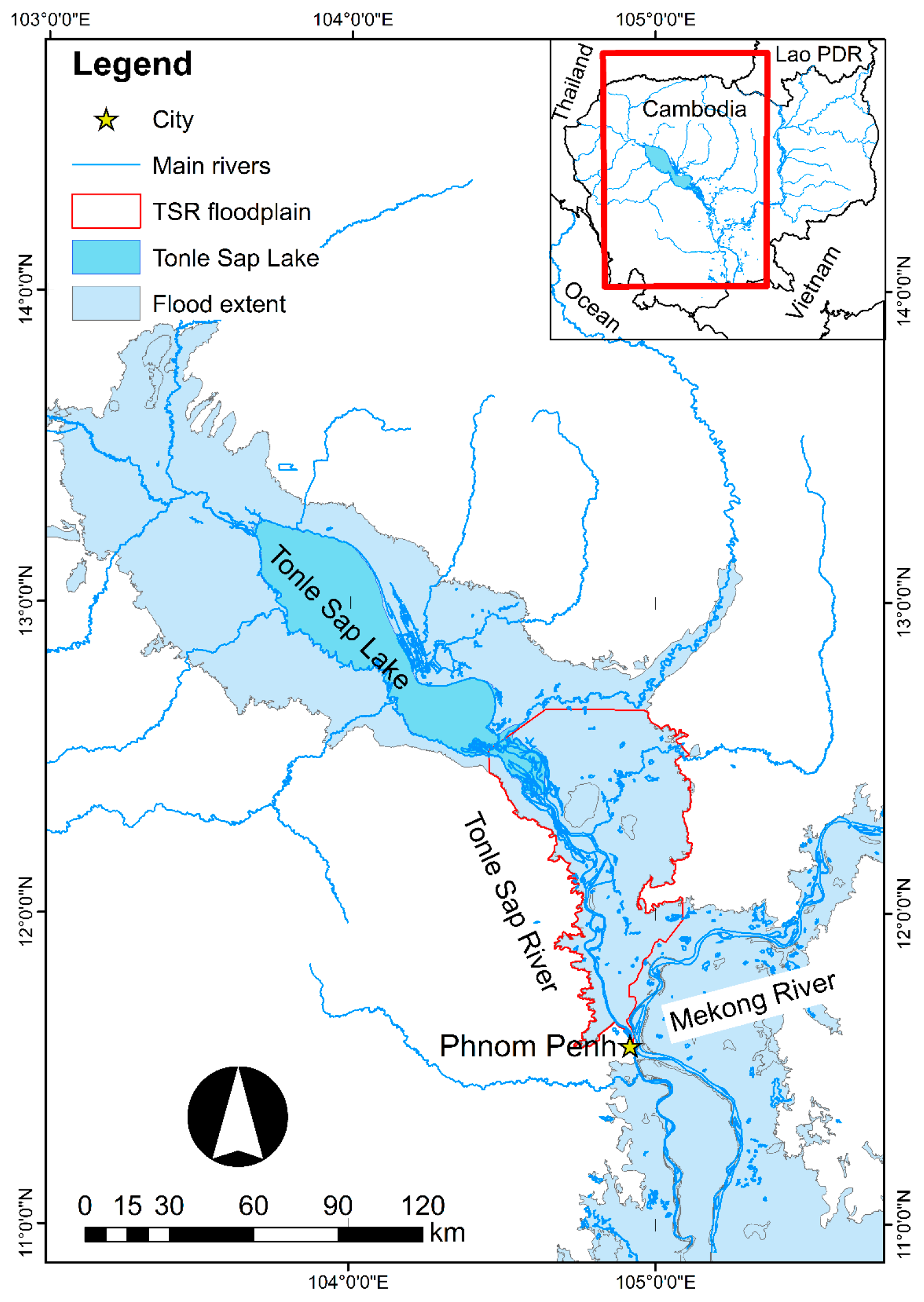
2. Study Area
3. Materials and Methods
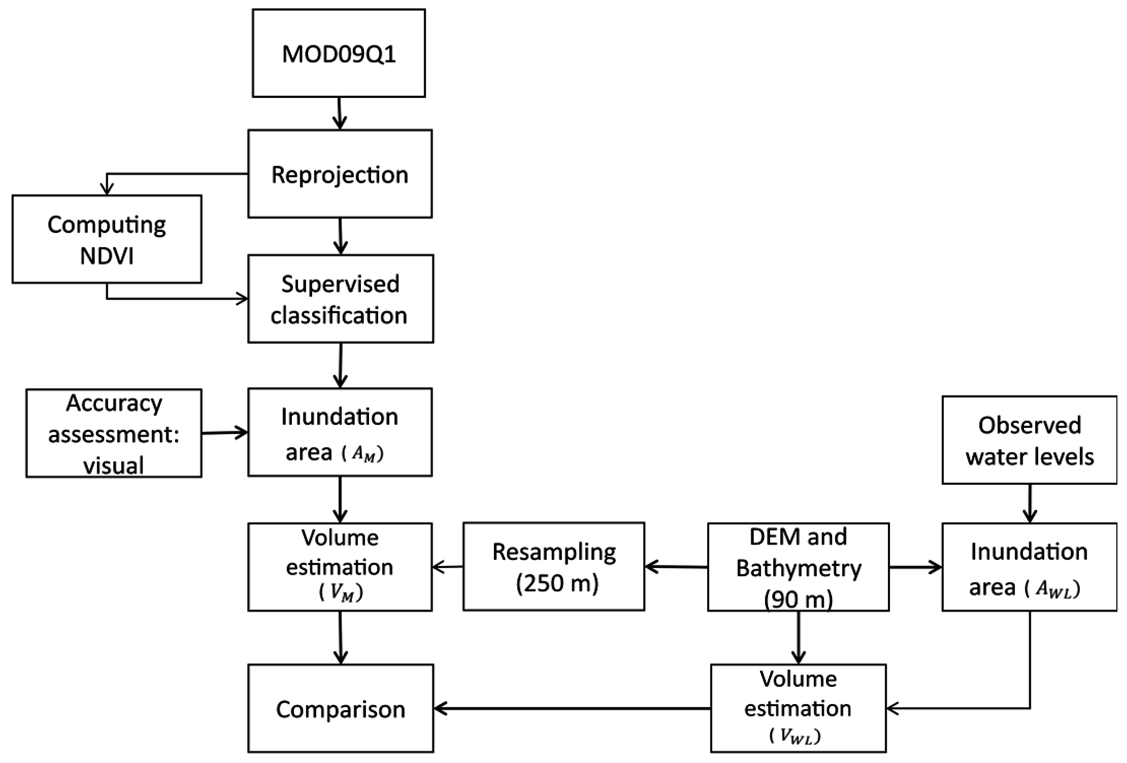
3.1. Inundation Mapping
3.2. Estimation of Water Volume
4. Results and Discussion
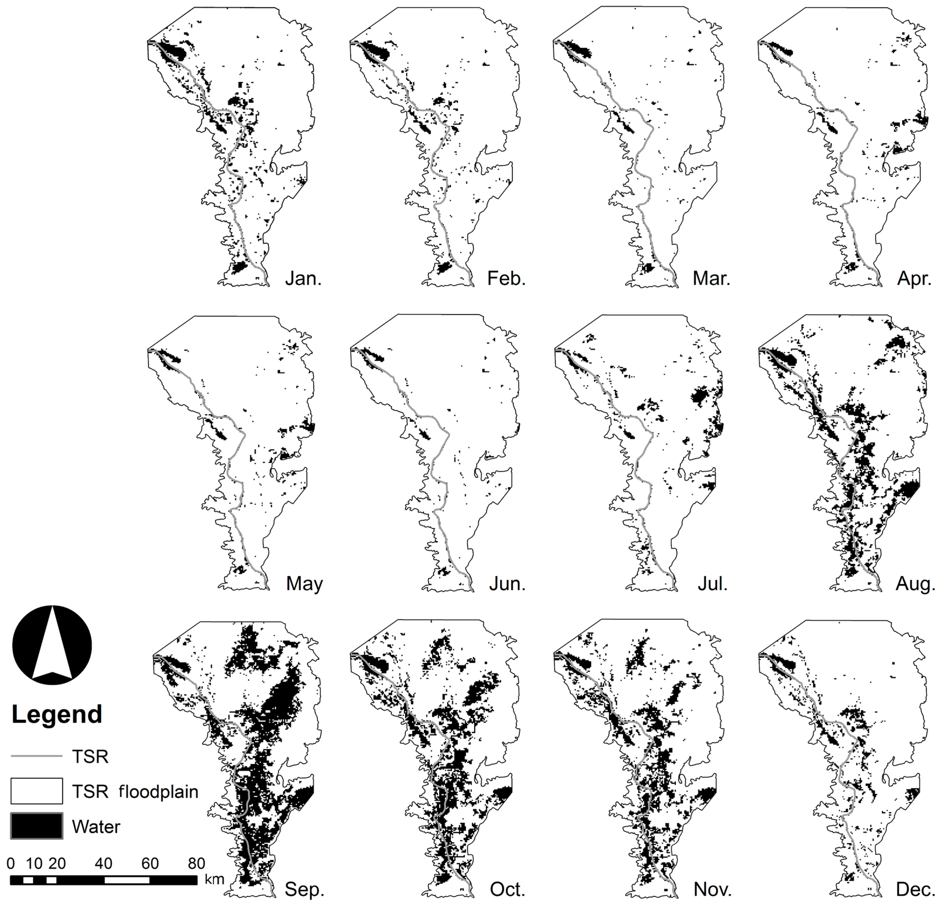
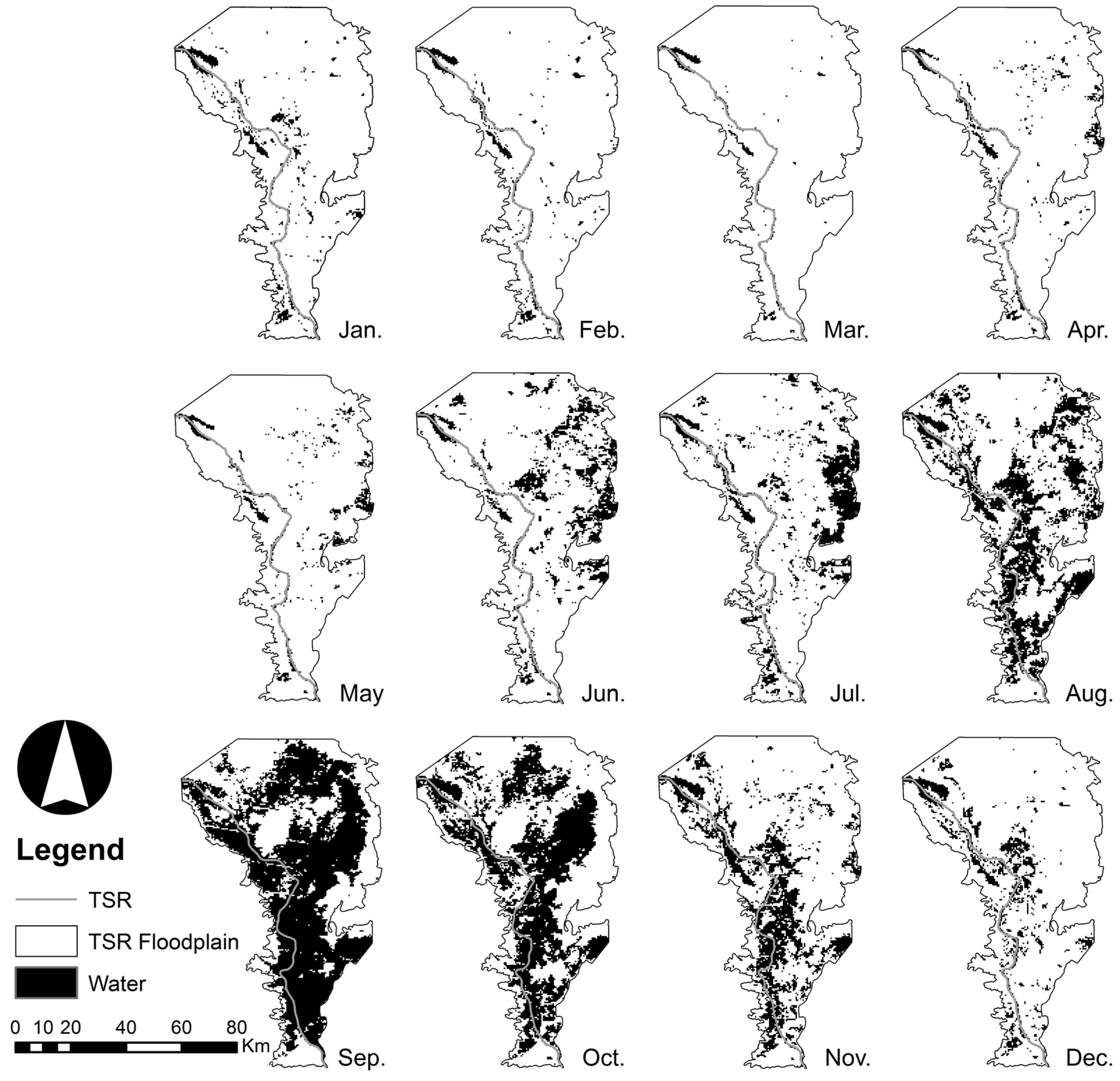
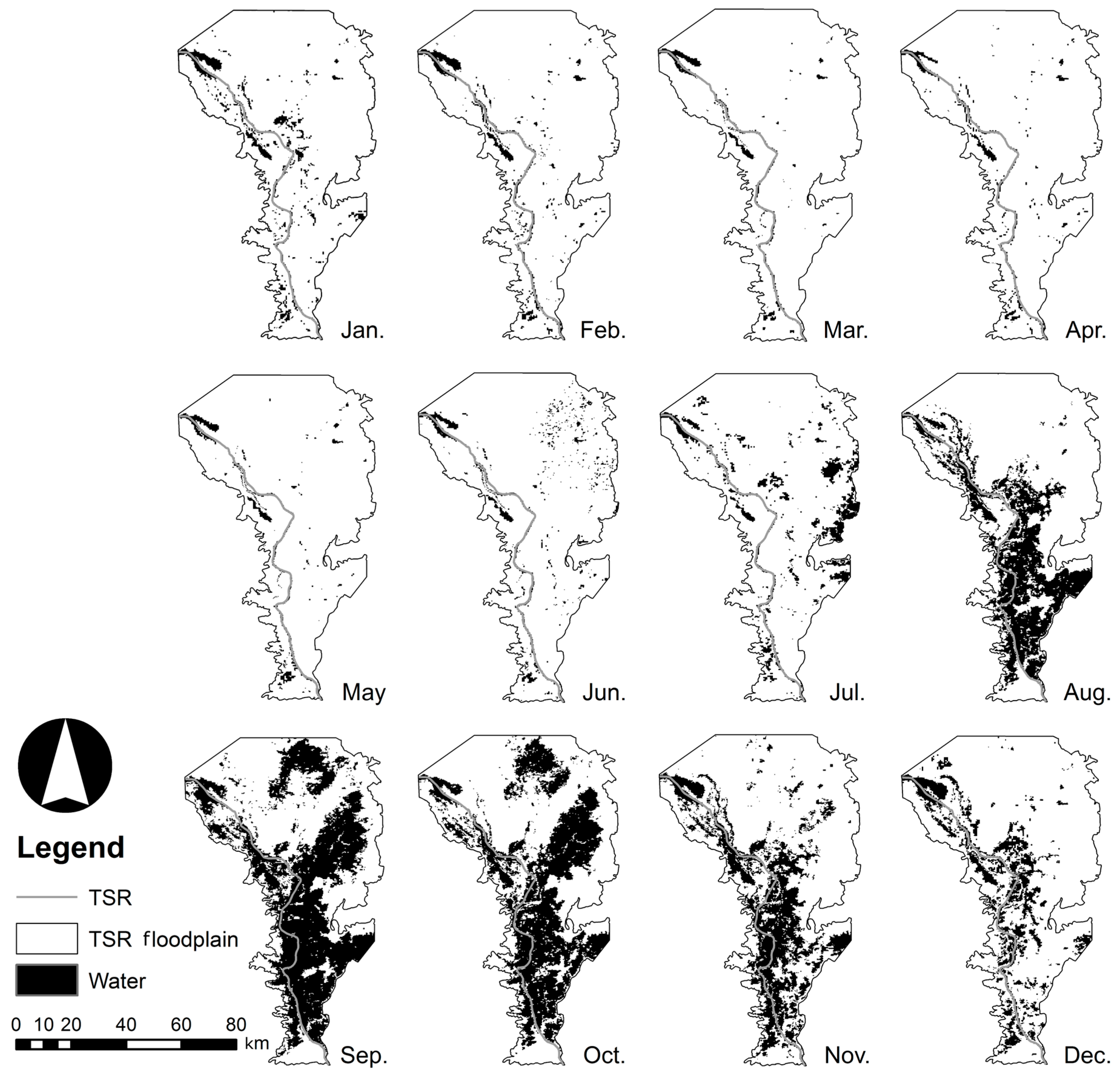
4.1. Inundation Area
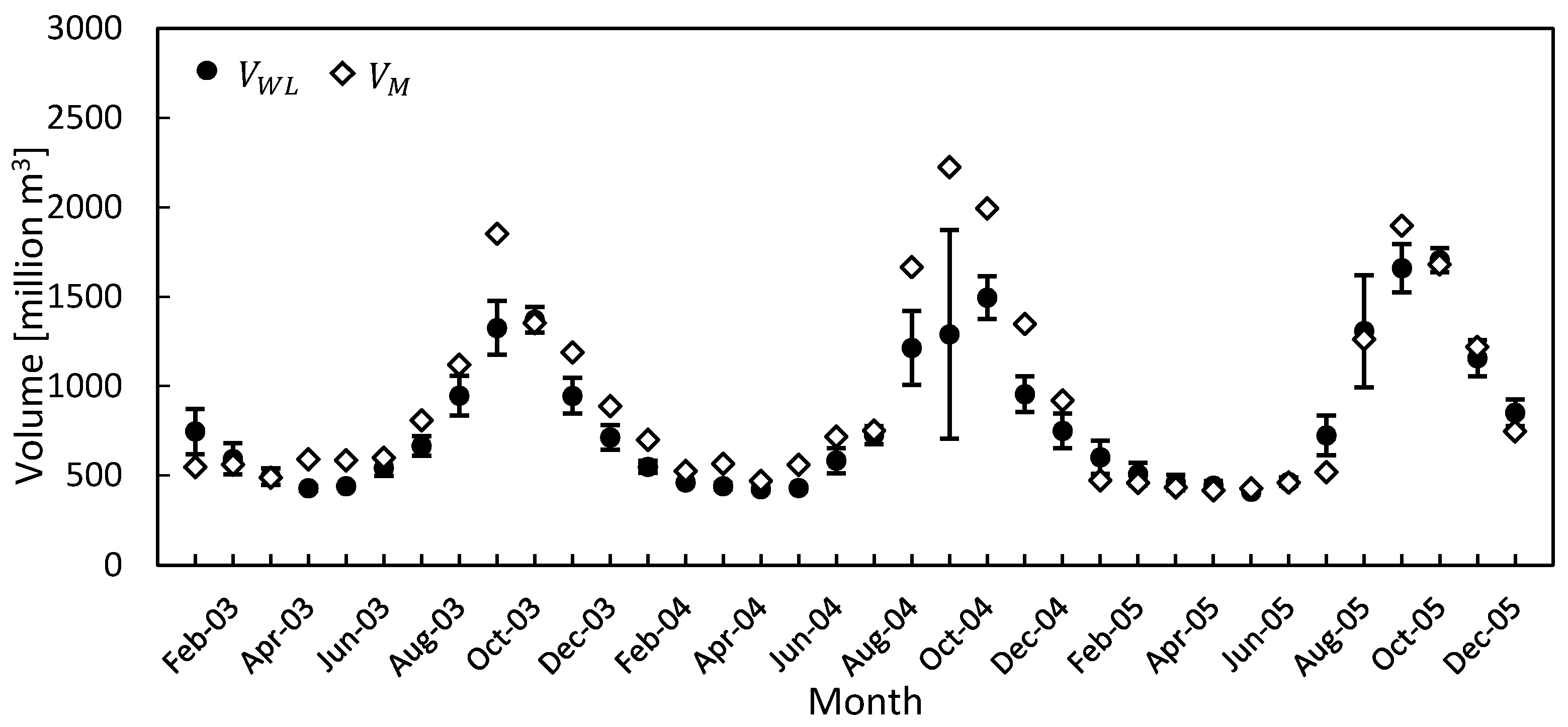
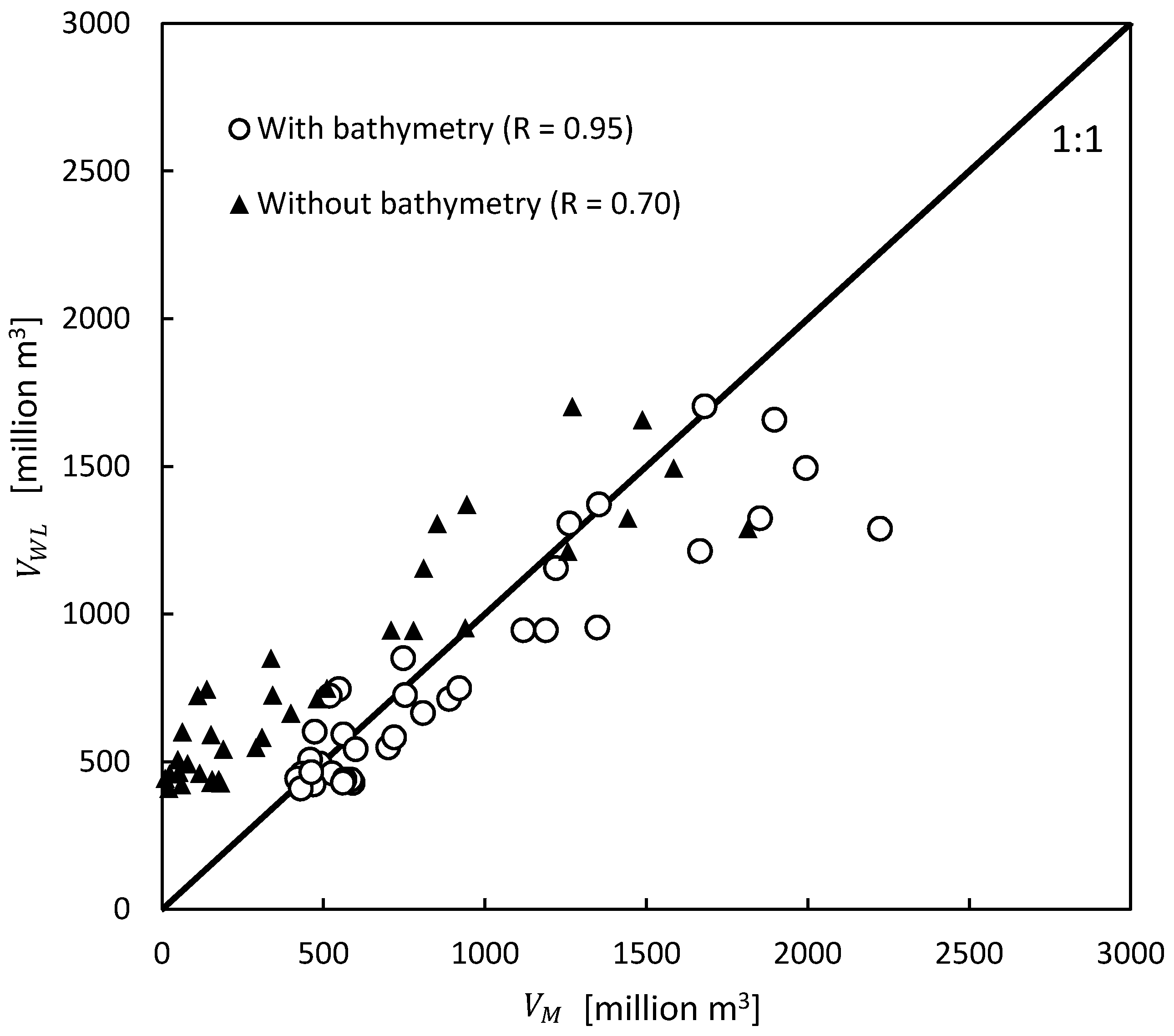
4.2. Water Volume in the Floodplain
5. Conclusions
Acknowledgments
Author Contributions
Conflicts of Interest
References
- Hudson, P.F.; Heitmuller, F.T.; Leitch, M.B. Hydrologic connectivity of oxbow lakes along the lower Guadalupe River, Texas: The influence of geomorphic and climatic controls on the “flood pulse concept”. J. Hydrol. 2012, 414, 174–183. [Google Scholar] [CrossRef]
- Junk, W.J.; Bayley, P.B.; Sparks, R.E. The flood pulse concept in river-floodplain systems. Can. Spec. Publ. Fish. Aquat. Sci. 1989, 106, 110–127. [Google Scholar]
- Tockner, K.; Malard, F.; Ward, J.V. An extension of the Flood pulse concept. Hydrol. Proc. 2000, 14, 2861–2883. [Google Scholar] [CrossRef]
- Lamberts, D. The Tonle Sap Lake as a Productive Ecosystem. Int. J. Water Res. Dev. 2006, 22, 481–495. [Google Scholar] [CrossRef]
- Ahmed, M.; Navy, H.; Vuthy, L.; Tiongco, M. Socioeconomic Assessment of Freshwater Capture Fistheries in Cambodia: Report on a Household Survey; Mekong River Commission: Phnom Penh, Cambodia, 1998; p. 186. [Google Scholar]
- Arias, M.E.; Cochrane, T.A.; Piman, T.; Kummu, M.; Caruso, B.S.; Killeen, T.J. Quantifying changes in flooding and habitats in the Tonle Sap Lake (Cambodia) caused by water infrastructure development and climate change in the Mekong Basin. J. Environ. Manag. 2012, 112, 53–66. [Google Scholar] [CrossRef] [PubMed]
- Hortle, K.G. Consumption and the Yield of Fish and Other Aquatic Animals from the Lower Mekong Basin; Mekong River Commission: Vientiane, Laos, 2007; p. 87. [Google Scholar]
- Lamberts, D.; Koponen, J. Flood pulse alterations and productivity of the Tonle Sap ecosystem: A model for impact assessment. AMBIO J. Hum. Environ. 2008, 37, 178–184. [Google Scholar] [CrossRef]
- Mekong River Commission. Basin Development Plan Programme Phase 2: Assessment of Basin-Wide Development Scenarios; Mekong River Commission: Vientiane, Laos, 2011; pp. 1–254. [Google Scholar]
- Chea, R.; Guo, C.; Grenouillet, G.; Lek, S. Toward an ecological understanding of a flood-pulse system lake in a tropical ecosystem: Food web structure and ecosystem health. Ecol. Model. 2016, 323, 1–11. [Google Scholar] [CrossRef]
- Kummu, M.; Tes, S.; Yin, S.; Adamson, P.; Józsa, J.; Koponen, J.; Richey, J.; Sarkkula, J. Water balance analysis for the Tonle Sap Lake-floodplain system. Hydrol. Proc. 2014, 28, 1722–1733. [Google Scholar] [CrossRef]
- Adamson, P. The Potential Impacts of Hydropower Developments in Yunnan on the Hydrology of the Lower Mekong. Int. Water Power Dam Constr. 2001, 53, 16–21. [Google Scholar]
- Laos; Nam Thuen II Power Company Ltd.; EcoLao; Norplan. Cumulative Impact Analysis and Nam Theun 2 Contributions: Final Report; Government of Lao PDR: Vientiane, Laos, 2004; p. 143.
- Arias, M.E.; Cochrane, T.A.; Kummu, M.; Lauri, H.; Holtgrieve, G.W.; Koponen, J.; Piman, T. Impacts of hydropower and climate change on drivers of ecological productivity of Southeast Asia’s most important wetland. Ecol. Model. 2014, 272, 252–263. [Google Scholar] [CrossRef]
- Cochrane, T.A.; Arias, M.E.; Piman, T. Historical impact of water infrastructure on water levels of the Mekong River and the Tonle Sap system. Hydrol. Earth Syst. Sci. 2014, 18, 4529–4541. [Google Scholar] [CrossRef]
- Johnston, R.; Kummu, M. Water Resource Models in the Mekong Basin: A Review. Water Res. Manag. 2012, 26, 429–455. [Google Scholar] [CrossRef]
- Kummu, M.; Sarkkula, J. Impact of the Mekong River Flow Alteration on the Tonle Sap Flood Pulse. AMBIO J. Hum. Environ. 2008, 37, 185–192. [Google Scholar] [CrossRef]
- Västilä, K.; Kummu, M.; Sangmanee, C.; Chinvanno, S. Modelling climate change impacts on the flood pulse in the Lower Mekong floodplains. J. Water Clim. Chang. 2010, 1, 67–86. [Google Scholar] [CrossRef]
- Reid, M.A.; Reid, M.C.; Thoms, M.C. Ecological significance of hydrological connectivity for wetland plant communities on a dryland floodplain river, MacIntyre River, Australia. Aquat. Sci. 2016, 78, 139–158. [Google Scholar] [CrossRef]
- Benger, S.N. Remote sensing of ecological responses to changes in the hydrological cycles of the Tonle Sap, Cambodia. In Proceedings of the IEEE International Geoscience and Remote Sensing Symposium 2007 (IGARSS 2007), Barcelona, Spain, 23–28 July, 2007; IEEE: Piscataway, NJ, USA; pp. 5028–5031.
- Fujii, H.; Garsdal, H.; Ward, P.; Ishii, M.; Morishita, K.; Boivin, T. Hydrological roles of the Cambodian floodplain of the Mekong River. Int. J. River Basin Manag. 2003, 1, 253–266. [Google Scholar] [CrossRef]
- Sakamoto, T.; Van Nguyen, N.; Kotera, A.; Ohno, H.; Ishitsuka, N.; Yokozawa, M. Detecting temporal changes in the extent of annual flooding within the Cambodia and the Vietnamese Mekong Delta from MODIS time-series imagery. Remote Sens. Environ. 2007, 109, 295–313. [Google Scholar] [CrossRef]
- Tangdamrongsub, N.; Ditmar, P.G.; Steele-Dunne, S.C.; Gunter, B.C.; Sutanudjaja, E.H. Assessing total water storage and identifying flood events over Tonlé Sap basin in Cambodia using GRACE and MODIS satellite observations combined with hydrological models. Remote Sens. Environ. 2016, 181, 162–173. [Google Scholar] [CrossRef]
- Van Trung, N.; Choi, J.H.; Won, J.S. A Land cover variation model of water level for the floodplain of Tonle Sap, Cambodia, derived from ALOS PALSAR and MODIS data. IEEE J. Sel. Top. Appl. Earth Obs. Remote Sens. 2013, 6, 2238–2253. [Google Scholar] [CrossRef]
- Mekong River Commission. MRCS/WUP-FIN Model Report: Modelling Tonle Sap Watershed And Lake Processes For Environmental Change Assessment; Mekong River Commission: Vientiane, Laos, 2003; p. 181. [Google Scholar]
- Arias, M.E.; Cochrane, T.A.; Elliott, V. Modelling future changes of habitat and fauna in the Tonle Sap wetland of the Mekong. Environ. Conserv. 2013, 41, 165–175. [Google Scholar] [CrossRef]
- Mekong River Commission. Overview of the Hydrology of the Mekong Basin; Mekong River Commission: Vientiane, Laos, 2005. [Google Scholar]
- Mekong River Commission/Information and Knowledge Management Programme. Final Report, Detailed Modelling Support Project (DMS); Finnish Environment Institute: Helsinki, Finland; EIA Ltd.: Espoo, Finland; Mekong River Commission (MRC) and Information and Knowledge Management Programme (IKMP): Vientiane, Laos, 2010. [Google Scholar]
- MRCS/WUP-FIN. Final Report—Part 2: Research Findings and Recommendations. WUP-FIN Phase 2—Hydrological, Environmental and Socio-Economic Modelling Tools for the Lower Mekong Basin Impact Assessment; Mekong River Commission: Vientiane, Laos, 2007; p. 126. [Google Scholar]
- Vermote, E.F.; Vermeulen, A. Atmospheric Correction Algorithm: Spectral Reflectances (MOD09); NASA: Washington DC, MD, USA, 1999; pp. 1–107. [Google Scholar]
- Xiao, X.; Boles, S.; Frolking, S.; Salas, W.; Moore, B., III; Li, C.; He, L.; Zhao, R. Landscape-scale Characterization of Cropland in China Using Vegetation and Landsat TM Images. Int. J. Remote Sens. 2002, 23, 3579–3594. [Google Scholar] [CrossRef]
- Rouse, J.; Haase, J.A.; Schell, J.A.; Deering, D.W. Monitoring Vegetation Systems in the Great Plains with ERTS, Proceedings of the 3rd ERTS Symposium, Washington DC, MD, USA, 10–14 December, 1973; NASA SP353: Washington DC, MD, USA, 1973; pp. 309–317.
- Spatial-analyst. Available online: http://spatial-analyst.net/ILWIS/htm/ilwismen/confusion_matrix.htm (accessed on 25 August 2016).
- Congalton, R.G. A Review of Assessing the Accuracy of Classifications of Remotely Sensed Data. Remote Sens. Environ. 1991, 37, 35–46. [Google Scholar] [CrossRef]
- Farr, T.G.; Rosen, P.A.; Caro, E.; Crippen, R.; Duren, R.; Hensley, S.; Kobrick, M.; Paller, M.; Rodriguez, E.; Roth, L.; et al. The Shuttle Radar Topography Mission. Rev. Geophys. 2007, 45. [Google Scholar] [CrossRef]
- Mekong River Commission. Hydrographic Atlas; Mekong River Commission: Vientiane, Laos, 2002. [Google Scholar]
- Lu, X.; Kummu, M.; Oeurng, C. Reappraisal of sediment dynamics in the Lower Mekong River, Cambodia. Earth Surf. Proc. Landf. 2014, 39, 1855–1865. [Google Scholar] [CrossRef]
- Li, R.-R.; Kaufman, Y.J.; Gao, B.-C.; Davis, C.O. Remote Sensing of Suspended Sediments and Shallow Coastal Waters. IEEE Trans. Geosci. Remote Sens. 2003, 41, 559–566. [Google Scholar]
- Deng, J.; Huang, X.; Feng, Q.; Ma, X.; Liang, T. Toward Improved Daily Cloud-Free Fractional Snow Cover Mapping with Multi-Source Remote Sensing Data in China. Remote Sens. 2015, 7, 6986–7006. [Google Scholar] [CrossRef]
- Hoan, N.T.; Tateishi, R.; Alsaaideh, B.; Ngigi, T.; Alimuddin, I.; Johnson, B. Tropical forest mapping using a combination of optical and microwave data of ALOS. Int. J. Remote Sens. 2013, 34, 139–153. [Google Scholar] [CrossRef]
- Li, S.; Sun, D.; Goldberg, M.; Stefanidis, A. Derivation of 30-m-resolution water maps from TERRA/MODIS and SRTM. Remote Sens. Environ. 2013, 134, 417–430. [Google Scholar] [CrossRef]
- Pan, F.; Liao, J.; Li, X.; Guo, H. Application of the inundation area—Lake level rating curves constructed from the SRTM DEM to retrieving lake levels from satellite measured inundation areas. Comput. Geosci. 2013, 52, 168–176. [Google Scholar] [CrossRef]
- Mekong River Commission. Annual-Mekong-Flood-Report-2011; Mekong River Commission: Vientiane, Laos, 2015; p. 72. [Google Scholar]


| Classification Methods | NDVI | MLC (Two Bands) | MLC (Two Bands + NDVI) |
|---|---|---|---|
| Accuracies (%) | 89.4 | 93.3 | 96.9 |
| Omission errors (%) | 10.6 | 6.7 | 3.1 |
© 2016 by the authors; licensee MDPI, Basel, Switzerland. This article is an open access article distributed under the terms and conditions of the Creative Commons Attribution (CC-BY) license (http://creativecommons.org/licenses/by/4.0/).
Share and Cite
Siev, S.; Paringit, E.C.; Yoshimura, C.; Hul, S. Seasonal Changes in the Inundation Area and Water Volume of the Tonle Sap River and Its Floodplain. Hydrology 2016, 3, 33. https://doi.org/10.3390/hydrology3040033
Siev S, Paringit EC, Yoshimura C, Hul S. Seasonal Changes in the Inundation Area and Water Volume of the Tonle Sap River and Its Floodplain. Hydrology. 2016; 3(4):33. https://doi.org/10.3390/hydrology3040033
Chicago/Turabian StyleSiev, Sokly, Enrico C. Paringit, Chihiro Yoshimura, and Seingheng Hul. 2016. "Seasonal Changes in the Inundation Area and Water Volume of the Tonle Sap River and Its Floodplain" Hydrology 3, no. 4: 33. https://doi.org/10.3390/hydrology3040033