
Plant-Based Methods for Irrigation Scheduling of Woody Crops

Group on Irrigation and Crop Ecophysiology, Instituto de Recursos Naturales y Agrobiología (IRNAS, CSIC), Avenida de Reina Mercedes, 10, 41012 Sevilla, Spain
Horticulturae 2017, 3(2), 35; https://doi.org/10.3390/horticulturae3020035
Submission received: 12 January 2017
/
Revised: 26 May 2017
/
Accepted: 26 May 2017
/
Published: 1 June 2017
(This article belongs to the Special Issue Refining Irrigation Strategies in Horticultural Production)
Abstract
:The increasing world population and expected climate scenarios impel the agricultural sector towards a more efficient use of water. The scientific community is responding to that challenge by developing a variety of methods and technologies to increase crop water productivity. Precision irrigation is intended to achieve that purpose, through the wise choice of the irrigation system, the irrigation strategy, the method to schedule irrigation, and the production target. In this review, the relevance of precision irrigation for a rational use of water in agriculture, and methods related to the use of plant-based measurements for both the assessment of plant water stress and irrigation scheduling, are considered. These include non-automated, conventional methods based on manual records of plant water status and gas exchange, and automated methods where the related variable is recorded continuously and automatically. Thus, the use of methodologies based on the Scholander chamber and portable gas analysers, as well as those of systems for measuring sap flow, stem diameter variation and leaf turgor pressure, are reviewed. Other methods less used but with a potential to improve irrigation are also considered. These include those based on measurements related to the stem and leaf water content, and to changes in electrical potential within the plant. The use of measurements related to canopy temperature, both for direct assessment of water stress and for defining zones with different irrigation requirements, is also addressed. Finally, the importance of choosing the production target wisely, and the need for economic analyses to obtain maximum benefit of the technology related to precision irrigation, are outlined.
1. Precision Irrigation
Precision agriculture began in the 1960s with the use of geographic information systems (GIS), probably the first precision farming tools developed. In the late 1980s and early 1990s, Global Positioning System (GPS) receivers became available for agricultural users interested in making sustainable decisions, and this was the origin of modern practices in precision farming. Within the context of precision agriculture, the aim of precision irrigation (PI) is to irrigate each plant with the right amount of water and at the right time, for optimal input use efficiency and minimum environmental impact [1]. Precision irrigation relies on an optimal combination of the irrigation system, the irrigation strategy and the irrigation scheduling method, as well as a wise choice of the production target. A huge variety of components are currently available on the market to adjust the irrigation system (furrow, sprinkling, localized…) to the conditions of any farm or orchard, such that the effective choice and implementation of the irrigation system is usually accomplished without major difficulties. In this work, therefore, the most demanding steps for PI, i.e., on the wise choice of the irrigation strategy, the method for the assessment of water stress and for irrigation scheduling, and the definition of the most appropriate production target, are considered.
Precision irrigation usually implies the use of deficit irrigation (DI), because of its potential to increase crop water productivity (WP) [2]. Achieving the greatest WP in a particular orchard implies a wise choice of the DI strategy. A variety of DI strategies have been defined, according to the amount and frequency of water supply (Table 1). Regulated deficit irrigation (RDI) is especially suitable for woody crops [3,4], including those in hedgerow orchards with high plant densities, currently considered among the most profitable management systems for fruit tree crops. The beauty of RDI is that it takes into account changes in the sensitivity of the crop to water stress at different developmental stages (e.g., as in Figure 1). This allows for maximum benefits of the supplied irrigation amounts. Regulated deficit irrigation, however, is challenging because it requires both a sound knowledge of the physiological response of the crop to water conditions and precise assessment of plant water stress levels along the growing cycle [5]. Thus, precision irrigation has not been a suitable approach for farmers and orchardists until recently, when enough knowledge on major processes related to the impact of environmental conditions on the development and production of crops has become available, and advances in sensoring, monitoring and data transfer have been made.
2. Irrigation Scheduling from Plant-Based Measurements
Plant-based measurements are widely used both to assess water stress and to schedule irrigation. Measurements related to soil water or atmospheric demand are also useful for irrigation scheduling, but the advantage of plant-based measurements relies on using the plant as a biosensor, which integrates the soil and atmosphere water status as well as the plant physiological response to the available water. Different methods based on the measurement of plant variables have been developed with the purpose of scheduling irrigation (Table 2). The most widely used methods are either conventional, non-automated methods for measuring leaf or stem water status, stomatal conductance or photosynthesis, or methods in which records are taken continuously and automatically, based on measurements related to sap flow, trunk diameter and leaf turgor pressure, among other variables [19,20]. The latter are those preferred for precision irrigation since, apart from running continuously and automatically, they can be implemented with data transmission systems for an easy and remote access to the recorded data through the Internet. In addition, those methods can be combined with remote imagery for the differential irrigation of zones within the orchard with different water requirements, which is one of the purposes of precision irrigation [21,22].
2.1. Non-Automated Methods
2.1.1. Stomatal Conductance
Plant transpiration (Ep) depends on the difference between the “effective” soil water potential at the root surface (Ψs) and the “effective” leaf water potential for the whole canopy (Ψl), and on the soil-plant hydraulic resistance (Rp), as shown in Equation (1) [25]:
Ep = (Ψs − Ψl)/Rp
A minimum Ψs − Ψl gradient (ΔΨ) must be achieved for water to flow from roots to leaves, thus allowing plant transpiration. During soil drying ΔΨ increases, leading to increasing tension in the xylem, i.e., the xylem water potential (Ψx) decreases. This may cause an increasing number of embolized xylem vessels, with the consequent loss of hydraulic conductance and increasing Rp [26]. The role of stomata is to regulate CO2 assimilation vs. water vapour loss. The loss of water through transpiration has the benefit of cooling down plants under high temperature conditions, but stomatal closure is required under drought to limit transpiration and avoid catastrophic xylem dysfunction [27]. Stomatal regulation of leaf gas exchange is, therefore, crucial for the survival of plants under arid and semi-arid conditions, i.e., when precipitation is below potential evapotranspiration. This relevant role of stomata is likely behind its high sensitivity and quick response to a great number of stimuli, including hormonal and hydraulic signals generated in roots and leaves, the water status in the immediate vicinity of stomatal guard cells, and vapour pressure deficit of the air, Da [28,29].
Stomatal aperture is measured as the stomatal conductance (gs), which is the inverse of the resistance offered by the stomata to the rate of passage of CO2 entering, or water vapour exiting, through the stomata. Stomatal aperture changes constantly, depending on changes in soil water status and atmospheric demand, among other variables, such that gs measurements are highly informative on the response of the plant to water stress. Thus, gs is considered one of the most effective water stress indicators in terms of earliness and sensitivity [30,31]. Measurements of gs can be easily made under field conditions by using porometers and infrared gas analysers (IRGAs) (Figure 2). The porometer can measure gs to water vapour while the IRGAs can measure gs to both water and CO2. Both devices have a chamber in which the whole leaf, or part of it, is enclosed during the measurement. If the cuticle is permeable to water vapour and CO2, the apparatus measures the leaf conductance (gl). If the leaf has an impermeable cuticle, the measurement yields the stomatal conductance (gs). Stomatal aperture depends markedly on the time of the day. The maximum daily stomatal conductance (gsmax), i.e., the gs value measured at the time of the day when stomatal opening is maximum, is widely used as a water stress indicator. When working with a species for which the daily dynamics of gs are unknown, daily curves of gs must be previously made to assess the time of the day at which gsmax must be measured [32]. In addition, information on the optimal environmental conditions leading to maximum potential gs values is valuable for properly assessing the meaning of field gsmax measurements [33].
Despite its significant potential as a water stress indicator, gs has limitations when used to schedule irrigation. First, both porometers and IRGAs must be operated manually, which limits the use of gs as a water stress indicator for precision irrigation. Recent advances, therefore, may change this. Hernandez-Santana et al. [34] reported a method to estimate gs from values of radial sap flux density and vapour pressure deficit of the air, two variables than can be continuously and automatically recorded under field conditions. Their findings show reliable estimations of gs, such that their approach opens the door for the use of gs as a water stress indicator in commercial fruit tree orchards under precision irrigation. Second, gs values are not always closely related to the plant water status. There are plants that are able to maintain a stable leaf water status over a wide range of atmospheric demand and soil water content. This is the case of the so-called isohydric species, which include maize and cowpea, among many others. In contrast, other species such as sunflower or barley are less effective at controlling leaf water status through stomatal closure, and they are termed anisohydric [35]. Some species such as grapevine may show isohydric or anisohydric behaviour, depending on the water stress conditions [29,36]. For other species, such as olive, a near-isohydric behaviour has been described, since they are able to keep relatively stable leaf water potentials but not as effectively as isohydric plants [37]. In the case of plants with isohydric behaviour, a significant decrease of gs occurs during the day while leaf water potential remains constant. The decrease of gs can be due not only to soil drying but to increasing atmospheric demand. Also, variability of water distribution in the rhizosphere, not only changes in the average available soil water, may cause significant changes in stomatal closure and thus in gs [5]. Further details on the efficiency of gs as a water stress indicator, depending on the isohydric or anisohydric behaviour of the plant, are given in the next section.
Finally, when using gs as a water stress indicator, it must be taken into account that the impact of stomatal closure on plant transpiration (Ep) depends on how well-coupled the crop canopy is with the atmosphere. Tall, rough canopies such as those of fruit tree orchards have aerodynamic conductances that are much greater than those of the short, smooth canopies of field and vegetable crops. Short canopies, particularly under low wind, are poorly coupled and offer much more resistance to mass transfer [38]. Under poor coupling, stomatal closure is less effective at controlling Ep because canopy temperature increases which, in turn, increases the vapour pressure gradient between the leaf and the atmosphere, increasing Ep. In well-coupled orchards, however, the greater heat transfer from leaves prevents large differences between canopy and air temperature, leading to a nearly linear relation between Ep and canopy resistance. Stomatal closure, therefore, will be more effective at reducing Ep in crops with tall canopies than in those with short canopies, particularly under low wind [2].
2.1.2. Leaf and Stem Water Potential
The plant water status is highly related to its performance, i.e., to growth, fruit size and fruit yield. It is not surprising, therefore, that a number of variables related to plant water status are being used as water stress indicators for irrigation scheduling. This is the case of predawn water potential (Ψpd), i.e., the water potential measured in the plant just before dawn, and leaf (Ψl) and stem water potential (Ψstem) measured at midday. The term “midday” refers here to the time of the day when minimum values of Ψl or Ψstem are recorded, which can be 2–4 h after solar noon [32]. That time is species-dependent and must be determined for the species of interest before using midday Ψl or Ψstem values for irrigation scheduling. Both Ψpd and leaf Ψl can be measured in single leaves. For the measurement of Ψl, well-developed, young leaves are sampled from outer, well-exposed locations of the canopy. In plants with tall canopies, leaves are usually sampled at about 1.4–1.7 m aboveground. During the night, differences in water potential within the plant are reduced, especially in plants that do not transpire at night, such that the location of the sampled leaf for the measurement of Ψpd is not so crucial. Still, leaves close to the base of the trunk are usually preferred for Ψpd measurements [39]. For Ψstem, either single leaves or shoot tips from the inner part of the canopy, close to the trunk or to a main branch, are wrapped in aluminum foil or enclosed in aluminum plastic bags some 1–2 h before sampling, to prevent transpiration [40,41]. Thus, the water potential of those leaves became similar to that in the xylem of the stem in the vicinity of the leaf or shoot attachment.
Measurements of Ψpd are hardly used in commercial orchards, because of the need of measuring before dawn. For Ψl and Ψstem, it is widely recognized that Ψstem could be a better indicator of water stress because it is less influenced by changing weather conditions than Ψl and, consequently, it shows less variability. The work by Garnier and Berger [42] is among the first studies reporting better performance of Ψstem than Ψl as a water stress indicator with potential for irrigation scheduling. Naor [40,43] also reported a greater sensitivity of Ψstem as compared to Ψl, from measurements in apple, nectarine, lychee, grapevine and Japanese plum, and a high correlation with fruit weight and yield. Naor [43] provided detailed information on the reliability of Ψpd and midday Ψl and Ψstem as water stress indicators. These three indicators are measured with Scholander-type pressure pumps, also called pressure chambers [44] (Figure 3). Measuring immediately after sampling is recommended, but this obliges transport of the Scholander chamber and related gear to the sampled plants, which can be both tedious and expensive. An alternative is to enclose the sampled leaf or shoot tip in an opaque container with wet paper inside, and keep it at low temperatures while being transported to the lab for measurement. Under these conditions of no light, air humidity close to 100% and low temperature, the sampled material can be kept for hours without significant change in water potential. Both Turner [45] and Hsiao [46] provided useful tips on the correct use of the Scholander chamber. Basically, the end of the leaf petiole or shoot tip should not be cut again before measurement. The flow of gas inside the chamber must be adjusted to ca. 0.1 bar s−1 (although the SI unit for plant water potential is the MegaPascal, or MPa, the bar unit is widely used for low water potential values; 1 bar = 0.1 MPa). If the material is severely stressed, the flow rate could be adjusted to an increase in pressure of 0.5 bar s−1, to shorten the measuring time. Greater rates of pressure increase within the chamber will lead to an increase in temperature and to errors due to the inertia between the increase in pressure and the appearance of water in the cut end, caused by the plant hydraulic resistance. It is also important to determine precisely the point at which water appears at the cut end. The wetting of the tissue, which must be observed with a magnifying lens, is enough. A dome of liquid water with bubbles coming out of the cut end means that the pressure inside of the chamber went too high.
Precautions must be taken when using the Scholander chamber in plants showing isohydric behaviour. Measurements of Ψpd provide information on the level of rehydration that the plant has achieved overnight. Therefore, Ψpd it is not influenced either by the isohydric/anisohydric behaviour of the plant or by daily adjustments of osmotic potential (Ψπ). The leaf water potential (Ψl), however, may be affected by both processes. Thus, neither Ψl nor Ψstem at midday are sensitive water stress indicators in plants showing isohydric behaviour, since the plant water status will change little despite significant changes in plant transpiration (Figure 4). For these plants, however, gs is very sensitive, since the stomata will close as soon as soil water decreases. The contrary can be said for plants with anisohydric behaviour: Ψl is a sensitive indicator of soil water depletion and gs is not. Both the capacity of osmotic adjustment and vulnerability to embolism of the sampled plant also have an influence on the sensitivity of Ψl as water stress indicator. The leaf water potential depends on the turgor (ΨP) and osmotic potentials, such that
Ψl = ΨP − Ψπ
Many species of arid and semi-arid areas have a large capacity for osmotic adjustment under soil-drying conditions, which allows the plant to keep high transpiration rates despite significant soil water depletion, since Ψl can reach low values before ΨP is markedly affected. This feature of reaching low Ψl values without affecting turgor pressure allows for keeping constant ΔΨ despite significant decreases in Ψs. This is an adaptive advantage for plants of semi-arid climates such as olive [47] since, according to Equation (1), it allows the plant to keep constant Ep values until a significant soil water depletion is reached (Figure 5). The plant transpiration (Ep) can also be defined in terms of canopy conductance (Gc), as
where Dl-a is the leaf-to-air vapour pressure deficit and P is the atmospheric pressure. Combining Equations (1) and (3) results in
with K as the hydraulic conductivity. The plant will limit Ep by closing stomata, i.e., by reducing Gc, before the loss of K reaches the limit for catastrophic hydraulic failure [27]. In species with a high capacity for osmotic adjustment, embolism will occur at a greater soil water depletion than in plants without such adaptive traits. In those plants, by the time the stomata finally close to avoid catastrophic hydraulic failure, water in the soil will be quite low and the recovery of the soil water status by irrigation will take longer.
Ep = Gc Dl-a/100P
Gc Dl-a/100P = ΔΨ K
Finally, there is a controversy in the scientific community on the meaning of the water potential measurements made with the Scholander chamber, described by Bentrup [48]. Basically, Zimmerman et al. [23] questioned whether the output of this tool, what they called the balancing pressure (Pb), reflects a 1:1 balance between the xylem tension in the intact plant, as it is widely recognized, and the chamber pressure. They stated that the actual tension in the xylem vessels cannot be as low as the values derived from the use of the Scholander chamber. Still, they acknowledged that the Scholander chamber is useful for detecting relative changes in turgor pressure. Zimmermann et al. [23] also claimed, in fact, that the cohesion–tension theory, widely accepted to explain the water ascent in plants, is misleading. Instead, they proposed the “multi-force” theory, which states that the ascent of water is not due just to the tension caused in transpiring leaves, but to forces of different kinds acting together. The user of the Scholander chamber, therefore, must take into account that the meaning of the output can be different depending on the approach adopted to explain the ascent of water in plants. An example is given by Fernández et al. [49] for the interpretation of measurements of Ψl in olive trees.
Both leaf and stem water potential can also be determined with thermocouple psychrometers (TCP). Although difficult to use in the field, mainly because of daily changes in air temperature, some TCP instruments can be used under field conditions [50,51]. Recently, a new type of small tensiometer has been developed for the measurement of water potential in plants. The device has a microelectromechanical (MEM) pressure sensor and a nanoporous membrane [52], and it is small enough to be embedded into plant stems to directly measure plant water potentials, down to about −10 MPa. According to the developers, this new technology has potential for automatic and continuous measurement of water potential in plants under field conditions.
2.1.3. Thermal Sensing
Measurements of canopy temperature (Tc) to assess water stress began some 50 years ago [54]. It was not until the development of the crop water stress index (CWSI, see below), however, that the method gained potential to schedule irrigation. Still, the method has been mostly used for research purposes only. Recently, however, the development of both cheaper image acquisition systems and user-friendly, powerful data image processing packages has substantially increased the potential of the method for irrigation scheduling in commercial orchards [55,56]. Thermal readings can be made both at the plant level (ground-based imagery) [55,57] and from above the crop (airborne imagery), after installing the sensors on towers or cranes [58,59], on unmanned aerial vehicles (UAVs), also known as remote piloted aerial systems (RPAS) [60], planes [61] or satellites [62,63]. Ground-based and airborne thermal images can be combined to assess within-orchard spatial heterogeneity in water status, as demonstrated with grape [64] and olive plants [65]. The principles of thermal sensing are described elsewhere [66,67] and nice examples on both the linking between thermal imaging to main physiological indicators [68] and the use of thermal imaging for irrigation scheduling [56,60,66,69] can be found in the literature.
Thermal sensing has two main constraints for precision irrigation. First, canopy temperature is related to leaf water status, but it also depends on radiation, air temperature, air humidity and wind speed, among other factors. Therefore, the use of Tc in the field as a water stress indicator requires normalizing Tc values relative to a reference. This can be done with the CWSI approach, as described in Equation (5) [24,70]:
CWSI = (Tc − Tnwsb)/(Tmax − Tnwsb)
In this equation, Tnwsb is the temperature of a non-water stressed reference crop under similar conditions, and Tmax is an upper temperature for a non-transpiring crop. Due to a number of inconveniences, which include the difficulty of having a non-transpiring crop reference, a number of alternatives to the CWSI have been proposed [71]. Still, both a Tdry and Twet temperature reference, representing a non-transpiring leaf and a fully transpiring leaf, are required. A variety of artificial and natural wet and dry surfaces have been used for empirical determination of Tdry and Twet [71]. Also, analytical methods for CWSI calculation have been proposed [58,67]. A second constraint of thermal sensing for precision irrigation is that full automation is not possible because of the need to process the thermal images. Despite those limitations, airborne imagery has a high potential for application to precision irrigation, since it allows for the zoning or zonification of farms and orchards, a process required for differential irrigation (Section 2.4).
The time of the day at which thermal images are taken has a great impact on the obtained information. This is because stomatal aperture changes dramatically during the day, influencing transpiration and thus leaf temperature (Tl). Also, the major weather variables related to both Tl and Tc change substantially along the day. If a single snapshot per day is taken, Ben-Gal et al. [58] recommended to take it at the time of maximum stress. They worked with olive trees, for which minimum daily values of Ψl were recorded in early afternoon. In general, the measurement of Tc by infrared thermometry is more advisable for field and row crops than for tree crops, because of differences on coupling between the canopies and the atmosphere and the impact on transpiration.
Ground-Based Imagery
Both infrared thermometers (IRT) and thermal cameras can be used for Tc readings. There are non-expensive, robust, wireless models of IRT that are installed in the field for collecting Tc readings with a frequency of seconds or minutes, and storing average values every minute or fractions of an hour [72,73]. Infrared thermometers perform better with low, homogeneous crops growing in regions with rather constant weather conditions [67]. Recently, however, the use of thermal cameras has become popular, thanks to lower prices and higher resolution. The best distance, angle, and time of the day at which the images should be taken must be checked for the crop conditions. Not only the species, but also the cultivar [74] and developmental stage [59] have an influence on the readings. The user must also bear in mind that relationships between thermal readings and water-stress-related physiological variables must be determined to properly evaluate the information provided by thermal imagery [66,75]. The literature provides examples on the use of ground-based thermal imagery to detect water status changes in a variety of plants, from ornamental [76] to herbaceous [59,77] and woody crops [57,68,78].
Airborne Imagery
As mentioned above, thermal images can be taken from unmanned aerial vehicles (UAVs), planes and satellites. Also, sensors mounted on a truck-crane have been used to monitor the whole orchard [79]. Airborne imagery is usually applied with two main purposes in this context, either to provide spatial distribution and variability of plant water status or to schedule irrigation. The first can help with the identification of zones within the farm or orchard with different sensitivity to water stress (zoning or zonification), and the selection of representative plants to be measured (Section 2.4). Agam et al. [79], for instance, assessed the spatial distribution of tree water status in an olive orchard, and suggested the procedure for choosing those trees best representing the orchard. The development of small, light, inexpensive thermal infrared (TIR) cameras, together with the appearance of low-cost, user-friendly unmanned aerial vehicles (UAVs), also known as remote piloted aerial systems (RPAS), has increased the applicability of airborne imagery to commercial orchards (Figure 6).
When thermal readings are taken with UAVs to assess the heterogeneity in water status within the orchard, flights are made around noon, on different days after an irrigation event, to detect increasing water stress differences among zones with different sensitivity to water stress. Examples are given by Gonzalez-Dugo et al. [21] for almond, apricot, peach, lemon and orange orchards, by Bellvert et al. [64] for a vineyard, by Gonzalez-Dugo et al. [22] for pistachio and by Egea et al. [65] for olive. Gago et al. [60] reviewed the use of different remote sensors providing a variety of indices (NDVI, TCARI/OSAVI and PRInorm), mounted on different types of UAVs, for sustainable agriculture. They cited key papers on the use of airborne imagery for assessing not only water stress variability, but also plant photosynthesis and the impact of crop diseases.
Most authors using thermal images taken from UAVs and planes reported robust relationships between the derived CWSI and main physiological variables related to water stress, such as stomatal conductance and stem or leaf water potential [56,64,65], and claimed that the approach was suitable for characterizing plant water status variability in woody crops. Remote sensing data acquired by satellite sensors can be used to derive daily evapotranspiration (ET) maps. Images from some satellites are free of charge, but both the return interval, about two weeks or more in some cases, and the spatial resolution, over 15 m for most satellites, are limiting for precision irrigation. The image downscaling method can be used to improve spatial resolution, such that ET maps for irrigation scheduling purposes can be derived [62]. Image fusion is also being proposed as a method to obtain higher spatial and spectral resolution images useful for irrigation management [63].
2.1.4. NIR Spectroscopy
The spectral reflectance of leaves in the visible to near-infrared (400–1100 nm) and infrared (1100–2500 nm) wavelength regions provides information on their water content. For whole canopies of plants under field conditions, near-infrared (NIR, 700–1100 nm) spectral indices are useful water stress indicators [80,81]. Thus, field-measured hyperspectral remote sensing data is being successfully used to estimate leaf water content and leaf water potential in vineyards [82,83,84,85], cotton fields [86] and maize [87], among other crops.
The principles of spectroscopy were well described by Cozzolino [88]. Basically, absorption frequencies can be used to identify specific chemical groups present in a vegetal sample. Thus, the relative proportions of C–H, N–H and O–H bonds of organic molecules can be identified by near-infrared (NIR) spectroscopy. The sample is irradiated with NIR radiation and the reflected or transmitted radiation is measured. Because water is a primary constituent of leaf tissues, the NIR reflectance spectra is dominated by the water spectrum, which shows overtone bands of the OH bonds at 760, 970 and 1450 nm and a combination band at 1940 nm [89]. Recent advances both in hardware (NIR spectrometers and related systems for data storage) and software (mathematical models for identifying different components in the spectrum of the sampled material, chemometrics) have allowed the development of on-the-go or in-field NIR spectroscopy methods for assessing plant water status, among other crop characteristics [85]. Although robust correlations between observed and predicted water potential have been reported [84,85,90], the price of the equipment, the cost of data acquisition (portable NIR spectrometers and related systems are usually mounted on vehicles than run through the orchard) and the need for substantial data processing are limiting factors for the use of this approach in a context of precision irrigation.
2.2. Automated Measurements
2.2.1. Sap Flow
A variety of methods have been developed for sap flow-related measurements, as detailed on the website of the Working Group on Sap Flow of the International Society for Horticultural Science (http://www.ishs.org/sap-flow/ishs-working-group-sap-flow-online-resources). The website provides a short description of the main methods, references to key papers, and a list of manufacturers, among other information. For the correct use of terms, units and symbols related to sap flow, the papers by Edwards et al. [91] and Lemeur et al. [92] are recommended. Sap flow-related measurements are widely used in research for in situ determinations of plant water consumption and transpiration dynamics (Figure 7), and their potential for irrigation scheduling has been assessed by Nadezhdina [93], Fernández et al. [94,95] and Jones [30], among others. Devices to schedule irrigation automatically from sap flow measurements have been designed and tested in fruit tree orchards [96,97], and comparisons with other methods to monitor plant water stress and to schedule irrigation have been made for a variety of crops, including apple [93], grapes [98], lemon [99], plum [100] and olive [101,102], among other species. In a recent review, Fernández [20] analysed the applicability of sap flow-related measurements for assessing water stress and irrigation scheduling in commercial orchards.
Sap flow sensors are robust and reliable enough for operation in the field over extended periods of time, and they are easily automated and implemented with data transmission systems. These features confer a high potential for use in precision irrigation. Yet their suitability for scheduling irrigation depends on the water stress indicator derived from the sap flow measurements. When the total plant sap flux is obtained with an invasive method (see the website mentioned above for differences between invasive and non-invasive sap flow methods), calibration of the raw data is required, for which correction factors must be previously derived for the species of interest [94,103,104]. In addition, a high number of sensors are usually required for trees with trunks of large diameter, because the azimuthal sap flow variability is usually high. The system becomes costly and time- and labor-consuming, and the user must be trained for the required data processing. These requirements curtail the use of this approach in commercial orchards. This explains the use of alternative water stress indicators derived from sap flow-related measurements. Nadezhdina and Čermák [96] used what they called the Sap Flow Index (see Nadezhdina [93] for details) to control irrigation in fruit tree orchards. Both Fernández et al. [94] and Nadezhdina et al. [105] suggested the possibility of using the ratio of sap flow in the inner/outer xylem regions as a trigger for when to irrigate. Recently, Hernandez-Santana et al. [34] developed an approach to derive stomatal conductance (gs) values from sap flow measurements. They demonstrated that it is possible to estimate gs in trees under field conditions, automatically and continuously, by using sap flux density (Jp) data directly, without the need for up-scaling to tree transpiration. They worked with olive, a species that has up to 3-year-old leaves. Basically, variations in the radial profile of Jp in the sapwood recorded in this species were attributed to a differential transpiration between younger leaves, better connected to the outer layers of the sapwood, and older leaves, better connected to inner sapwood. In addition, Jp data were taken at two depths only below the cambium (at 5 and 10 mm), instead of the four depths required when the system is used in a standard way. As mentioned in Section 2.1.1, this new approach may favour an increasing use of sap flow measurements in orchards under precision irrigation.
2.2.2. Stem and Fruit Diameter
After stomatal opening early in the morning, a tension is created from the evaporative surface of the leaves to any water-storing organ of the plant, i.e., to the stem, branches, roots, leaves, and fruits [106,107,108]. Water stored in the tissues during the night is then lost, allowing the plant to respond rapidly to changes in atmospheric demand, prior to water uptake by the roots [109]. Thus, water from the phloem and related tissues, as well as from the living tissues of the sapwood, is lost by transpiration, so that the stem diameter decreases [110,111,112]. Changes in the water content of extensible tissues of the stem are readily reversible, such that later in the day and during the following night, the plant rehydrates and stem diameter increases. This causes stem diameter variation (SDV). In trees, daily SDV usually ranges from a few tenths to a few hundred microns, depending, among other factors, on stem diameter and wood elasticity [113,114]. For some purposes, it may be advisable to convert the SDV data to areas and normalise by the initial area in order to obtain comparable, size-independent measurements of daily dimensional changes [115].
On days of high soil water availability and low atmospheric demand, and when the plant is in a period of active growth, stem diameter increases from one morning to the next, with little, if any, decrease during the day. If both the soil water availability and the atmospheric demand are high, stem diameter also increases from one morning to the next, but an appreciable decrease could take place during the day, as a result of plant growth and tissue dehydration in the morning and rehydration after stomatal closing later in the day. On days when the soil is dry and the evaporative demand is high, there is a reduction in stem diameter, with only a partial recovery during the night. Under those conditions, the stem diameter can remain stable or even decrease from one day to the other, because the plant does not grow and becomes increasingly dehydrated [109,116,117]. The work by Herzog et al. [118] gives additional information on the diurnal dynamics of SDV, and how it is related to the diurnal dynamics of transpiration.
Different water stress indicators can be derived from the resulting daily patterns of SDV, as summarized in Table 2. For details, see Goldhamer and Fereres [119], Gallardo et al. [120], Fernández and Cuevas [113] and De la Rosa et al. [121], among others. For scheduling irrigation, the maximum daily shrinkage (MDS) and stem growth rate (SGR) are the most widely used of these indicators. Values of MDS, however, must be used with care since, for some species, the MDS vs. Ψstem relationships show diurnal hysteresis (lag) and seasonal changes. Also, and very important, for some species MDS increases as the plant water potential falls to a certain value, after which MDS decreases as the plant water potential becomes more negative. This has been reported for peach, lemon, grapevine and olive, among other species [114]. On the other hand, SGR cannot be used as an indicator of plant water stress in periods of negligible growth, for instance in grapevines after veraison (ripening) [122]. Thus, expert interpretation of SDV records is required before using them for scheduling irrigation, which limits their potential for automating the calculation of the irrigation dose [20].
Additional complications in data interpretation come from the fact that the patterns of SDV are affected not only by environmental water conditions and growth patterns, but also by plant age and size, and crop load, among other factors. For young trees, and in periods of rapid stem growth, SGR could be a better indicator than MDS. This is because MDS, for those trees and conditions, could be affected more by growth than by the level of water stress. This has been observed in peach [119], olive [123], lemon [124], and almond [125], among other species. On the other hand, in periods of negligible growth because of active fruit development, SGR is not a reliable indicator of plant water stress. This has been observed in grapevines [122], plum [126], and olive trees [127]. The seasonal growth patterns of any plant also depend on the crop load, so this is another factor influencing SDV records. In olive trees, a species with marked alternate bearing, trees with heavy fruit load (‘on’ year) exhibited the most-active trunk growth until some four weeks after full bloom, and grew very slowly for the rest of the season, while trees with a light crop load (‘off’ year) grew steadily throughout the season at an increasing rate [128]. In plum trees, Intrigliolo and Castel [129] found that during most of the fruit growth period, when SGR was minimum, MDS was higher in the less-irrigated treatment than in the control, and correlated well with Ψstem. After harvest, however, when SGR was higher, the MDS vs. Ψstem correlation decreased as the season progressed. De Swaef et al. [130] provided an explanation on the effect of crop load on MDS and daily growth rate (DGR) in peach, with the help of a water and carbon transport model. The use of models to interpret SDV records was reviewed by De Swaef et al. [131]. Other factors have been also been identified as influencing SDV records. Thus, Intrigliolo and Castel [129] suggested an influence of the soil volume wetted by irrigation, and Gallardo et al. [120] found that the signal values of MDS recorded in potted pepper plants in a greenhouse were greater those in soil-grown pepper plants, and suggested that the small rooting volume of pots favoured that response. Also, Silber et al. [132] suggested that the water-stress history of avocado trees, rather than the actual plant-water status, could have influenced maximum trunk diameter variation (MTDV).
Despite difficulties in data interpretation, SDV has a potential application for precision irrigation because the current dendrometers and related systems are robust and precise, suitable for automatic recording and data transmission under field conditions (Figure 8). The first highly sensitive dendrometers and dendrographs were developed in the late 1800s [133,134] but it was not until the second half of the last century when technological advances allowed for precise SDV measurements [135,136,137]. From the beginning of the 1990s, most authors working on irrigation scheduling have used linear variable differential transformers (LVDT), also called linear variable displacement transducers. The LVDT-type sensors are robust and of high precision, close to ±1 µm. In many cases, however, the resolution cannot be expected to be greater than about 10 µm, due to errors associated with calibration, voltage recording, temperature changes, and other factors [129]. Ueda et al. [138] reported advantages (small size, light weight, low price, ease of use, and reliability) of the strain-gauge method over the LVDT-type sensor for estimating diurnal changes in stem and branch diameters of a large tree. The method was also used by Ueda and Shibata [106].
Some dendrometer models are nailed or screwed into the tree, either to support the instrument or to serve as a fixed reference against which growth is measured. Others are mounted on a holder that is attached tightly to the stem by elastic straps, which do not affect growth. Holders are usually of aluminum and INVAR, an alloy of Fe and Ni with negligible thermal expansion. In fruit trees and other plants of large stem diameter, dendrometers are installed on the side of the stem opposite to the sun’s trajectory, to minimise negative effects of heating by direct solar radiation. They must be at a certain distance from the ground to avoid interference from growing weeds, and far from scars and other irregularities of the trunk surface. The outer, dead tissues of the bark must be removed before installation, allowing the contact point of the sensor to rest directly on the living tissues of the bark. The dendrometer must always be in contact with the plant surface, for which a spring or glue can be used, and the whole area must be covered with insulating material and reflective thermoprotecting foil to minimise both heating by direct solar radiation and the impact of rain drops. Recommendations on dendrometer installation are given elsewhere [113]. Once installed, the dendrometer is connected to a data logger programmed to automatically scan the sensor outputs every few seconds and store average values every few minutes. The data logger is usually provided with a system for data transmission. After installation the dendrometers can run for months or even longer with practically no maintenance. Still, LVDTs are particularly prone to obstruction by insects.
Different devices have been built to schedule irrigation from SDV records. Pelloux et al. [139] described the Pepista system marketed by the French company Agro-Technologie (www.agro-technologies.com), and Bussi et al. [140] used it to control irrigation in a 10-year-old peach orchard. Other companies, such as the Spanish Verdtech (www.verdtech.es) and the Israeli Phytech (www.phytech.com), have developed automatic monitoring systems of SDV records. Examples of different approaches to scheduling different irrigation strategies from SDV records have been recently published for olive [141,142,143,144]), nectarine [121] and peach [145,146], among other species. These publications, together with that by Fernández [20], describe well the potential and limitations of the use of SDV records for irrigation scheduling.
Contrary to use of SDV records, on which a large number of papers have been published, those on the use of fruit diameter as an indicator of water stress are very few. The first attempts to correlate changes in fruit diameter with environmental conditions for non-destructive estimates of water stress useful for irrigation scheduling, were made in the 1960s and 1970s [147]. Devices range from digital calipers used manually [148,149] to automatic devices for accurate, continuous measurements [150]. Recording fruit diameter is useful for studies on the impact of irrigation and other management and environmental factors on fruit production. Little attention has been dedicated, however, to the use of this approach for irrigation scheduling in commercial orchards.
2.2.3. Leaf Thickness
There is evidence of changes in leaf thickness in relation to soil and atmosphere water status, suggesting a potential for plant water stress assessment [151,152]. Leaf thickness-related measurements are made with devices containing linear potentiometer transducers (same principle as LVDT measurements). The method is non-invasive and suitable for online measurements. It seems that the method is more suitable for crops under cover, since wind in open field crops causes noisy records. Another disadvantage is that relationships between leaf thickness and leaf water status are not robust. They depend on the species, leaf type and age, stress history and other factors [153]. In addition, recent findings published by Seelig et al. [154] showed a lack of correlation between leaf thickness and turgor pressure. Still, devices to schedule irrigation from leaf thickness-related measurements have been developed and tested in cowpea plants under greenhouse conditions [155] and in citrus, avocado and cotton crops under open field conditions [156]. An additional problem for the use of the system in commercial farms and orchards is that, depending on the species and leaf-width gauge model, the user could be required to reinstall the sensors in new leaves quite often [157].
2.2.4. Leaf Turgor Pressure
Leaf turgor has a significant effect on stomatal behaviour and, thus, on plant water status and water consumption. Rodriguez-Dominguez et al. [158] measured drought responses of variables related to water stress in three important woody species in the Mediterranean climate (almond, grapevine and olive), and, with the help of a process-based gs model, found that responses mediated by leaf turgor could explain over 87% of the observed decline in gs across species. They used the stomatal model of Buckley et al. [159], also known as the BMF model, which is based on the hydroactive feedback hypothesis (HFH). That hypothesis states that guard cell osmotic pressure depends markedly on leaf turgor. The HFH hypothesis is supported by sound evidence, including a recent discovery by McAdam et al. [160] on a molecular mechanism for negative feedback regulation of guard cell osmotic pressure by leaf turgor. The close relation between gs and leaf turgor supports the utility of leaf turgor-related measurements as a valid indicator of water stress.
Measurements of turgor pressure in cells and xylem vessels can be made with sophisticated equipment requiring well-trained users, and include methods such as the ball tonometry method [161] and the pressure probe technique [23]. Recently, Zimmermann et al. [162] developed the magnetic leaf patch-clamp pressure probe, known as the LPCP or ZIM probe (Figure 9), for leaf turgor pressure-related measurements under field conditions. Briefly, the probe consists of two metal pads in which two magnets are integrated. One of the patches also contains a pressure-sensing chip. The patches are located in the adaxial and abaxial sides of a leaf, such that the pressure chip is in close contact with the leaf surface. The distance between the magnets above and below the clamped leaf patch is adjusted according to the rigidity and elasticity of the leaf, by regulating the distance between the two magnets. The leaf turgor pressure (Pc) is determined by measuring the pressure transfer function through the leaf. The attenuation of the applied external pressure and, thus, the output pressure signal (Pp) provided by the ZIM probe, depends on the magnitude of Pc. High Pc attenuates the pressure transfer through the leaf patch and, in turn, Pp is small. Therefore, Pp is inversely correlated with Pc. The ZIM probes are connected by cable to a radio transmitter (telemetric unit), which sends the collected data to a data logger (controller) implemented with a GPRS modem linked to an Internet server via the local mobile phone network. From the server, the data can be downloaded by smartphones, tablets and laptops. Thus, the collected data are available for the user in nearly real-time. If desired, the system can also measure air temperature, relative humidity and light intensity close to the plant, as well as soil temperature and moisture [163].
The ZIM probes work well in hydrated and moderately hydrated leaves. Above a certain level of dehydration, air and vapour accumulates in the leaf tissues and the pressure chip does not properly sense the turgor pressure. The extent to which this limitation curtails the potential of the ZIM probes to monitor water stress was assessed for olive by Fernández et al. [49] and Ehrenberger et al. [164]. Other effects of the environmental conditions and plant hydraulic functioning on the performance of the ZIM probe, were detailed by Zimmermann et al. [163]. The ZIM system has been tested in a variety of forest tree species [165], grapevines [166,167], and grapefruit [167], banana [168], persimmon [169] and olive trees [49,170,171,172], as well as in herbaceous crops such as tomato [173], canola [174] and wheat [175,176]. Also, comparative studies of the ZIM system vs. Scholander-type chambers have been made by Westhoff et al. [166] for grapevines, by Rüger et al. [165] for eucalyptus, avocado, grapefruit, beech and oak, and by Ben-Gal et al. [170] and Fernández et al. [49] for olive. These studies showed that the ZIM system is robust, relatively inexpensive, and suitable for automatic and continuous recording under field conditions for long periods of time, and that it has a great potential as a water stress indicator in vineyards and fruit tree orchards. Padilla-Díaz et al. [7] used it successfully to schedule a regulated deficit-irrigation strategy in a hedgerow olive orchard with high plant density.
Leaf turgor pressure can also be estimated with the Wiltmeter [177], a portable instrument for leaf turgor-related measurements suitable for working under field conditions. Earlier versions had some limitations, detailed by Aroca and Calbo [178], such that an R2 version was developed for simpler portable operation on the field [179]. This version, however, still required user intervention, and measurements were influenced by the way the user operated the system. Recently, two new versions of the Wiltmeter have been released [178], which allow automated turgor pressure measurements at user-defined logging intervals. According to the authors, the new Wiltmeter can be used for both ecophysiological studies and irrigation scheduling, but, to our knowledge, no evidence of the latter has yet been published.
2.2.5. Stem Water Content
The principles of dielectric methods to measure water content in a medium are given elsewhere [180]. Basically, the water content and electrolyte concentration of a medium can be accurately determined from the measurement of its dielectric properties. Water has a high dielectric constant (ε) of about 80, much higher than that of the air (ca. 1) or the dry constituents of many mediums (for dry soil, ε is about 5). Two methods have been developed based on the measurement of dielectric properties, one in the frequency domain between 30–3000 MHz and the other in the time domain at frequencies above one GHz. Time domain reflectometry (TDR) sensors are based on the latter. The principle of the technique is thoroughly explained by Topp and Davis [181]. Measuring stem water content (θstem) by TDR assumes that soil water drying induces significant changes in the water content of tree stems. It is known that stems of many tree species undergo substantial seasonal variations in θstem [182] and that water storage in the sapwood can make a significant contribution to daily transpiration under periods of high evaporative demand [183]. By measuring θstem with TDR in aspen, piñon, cottonwood and ponderosa pine trees, Constantz and Murphy [184] found absolute values for θstem between 0.20 and 0.70 L L−1, with an annual change in moisture content between 15% to 70%, depending on the species and water environmental conditions. Results of this type have been reported for many other species, as detailed by Nadler et al. [157]. These authors used a TDR methodology to measure electrical conductivity in the stem of mango trees under changing water and salt conditions. They found that stem electrical conductivity (σstem) was primarily dependent on θstem and only negligibly on stem cell salinity, and concluded that stem resistivity measurements could be used to represent dielectric changes in the stem. In a later study, they focused on a more user-friendly and less expensive tool, after stating that TDR was too expensive and complicated for commercial orchards. They studied the relations between σstem and θstem, both in tree stem segments [185] and in lysimeter-grown mango, banana, date and olive trees [186] (Figure 10), and confirmed that θstem reacts sensitively and within minutes to water stress. They proved that resistivity measurements have lower scatter because θstem vs. ε relationships are exponential and θstem vs. σstem relationships are linear. Also, the resistivity measurements were easier to make than the ε measurements, and allowed for smaller probes, longer cables, simpler multiplexing and a lower price, among other advantages. They concluded that there is a clear economic advantage in resistivity over ε measurements, and that the monitoring of σstem has a potential in scheduling irrigation in fruit tree orchards. An example of the applicability of the method in vines was published by Coskun and Konukcu [187]. They analysed the correlation between volumetric soil water content and σstem, and concluded that further experiments on the suitability of σstem measurements to both monitor water stress and schedule irrigation were needed to properly evaluate the performance of the methodology when applied to vines. To our knowledge the method has not been automatized yet, but authors claimed that automation is possible.
2.2.6. Electrical Potential
Stomatal closure can be triggered by long- and short-distance signaling, involving signals of different natures [188,189]. Although most studies focus on signals of chemical or hydraulic nature, electrical signaling has received increasing attention in recent years. Although the first extracellular electrical measurements in plants date from the 19th century [190], Fromm and Eschrich [191] were among the first to hypothesize that changes in the electrical signals might be a mechanism of communication between roots and leaves. Since then, an increasing amount of evidence suggests that the bioelectric potential in plants is affected by a variety of environmental changes, including soil water availability. In work with maize plants, Fromm and Fei [192] observed that sieve tubes of the phloem serve as a pathway for electrical signal transmission from roots to leaves. In avocado trees, Gil et al. [193] found that changes in extracellular electrical potential between the leaf petiole and the base of the stem (ΔVL-S) may play a role in root to shoot communication when plants are under water stress. They outlined the need for separating true electrical signaling phenomena from conductivity changes arising from water or ion handling by the plant tissue, and concluded that changes in ΔVL-S may be a mechanism for root to shoot communication leading to stomatal closure in response to soil drying. Gurovich and Hermosilla [194], Gil et al. [195] and Oyarce and Gurovich [196] found that electrical signaling resulting from microenvironment modifications can be quantitatively related to the intensity and duration of the stimuli, as well as to the distance between the stimuli site and the location where electric potential is measured. They suggested the existence of a sort of proto-nervous system in plants, in agreement with suggestions made by other groups working on the subject [197,198,199].
Gurovich and Hermosilla [194] described a digital acquisition system for recording ΔVL-S with microelectrodes inserted 15 mm deep into the sapwood at various positions in the trunks of avocado, blueberry, lemon and young olive plants in pots (Figure 10), and discussed the potential of using ΔVL-S patterns, during day-night cycles and at different conditions of soil water availability, as tools to assess early plant water stress conditions. A different system was described and tested in cucumber plants under greenhouse conditions by Wang et al. [200]. Recently, Ríos-Rojas et al. [201,202] developed a system for remote, real-time recording of plant electrical potential in the field and data transmission via Internet. The authors concluded that their system could be used to monitor water stress and, combined with soil moisture and potential evapotranspiration sensors, to schedule irrigation.
2.3. The Combined Use of Methods
The potential of combining sap flow (SF) and trunk diameter variation (TDV)-related measurements to assess water stress has been evaluated for a variety of species [108,113,203]. The approach allows for deriving water stress indices [101,102], as well as modeling tools [204,205] for irrigation scheduling of fruit trees. Drew and Downes [206] and Fernández and Cuevas [113] reported main factors explaining agreements and disagreements between concomitant records of SF and TDV in the same plants. There is a consensus on the potential of the combined use of these two methods to better understand the water-flow dynamics within a plant [108,203,204,205,207] and to assess both water stress [102] and water needs [101]. Also, the combined use of SF and eddy covariance measurements is useful for assessing the partition of ET fluxes [208,209,210] and to derive crop coefficients for irrigation scheduling [211]. Eddy covariance [212] and satellite observations [213] have also been combined with soil water balance simulations to derive the value of basal crop coefficients for the dual crop coefficient approach. Other examples relying on the use of combined measurements are provided by Centeno et al. [214] and Cancela et al. [215], who suggested combining measurements of soil water and plant water status to improve irrigation management in vineyards.
Additional examples on the joint use of two or more methods to gain insight into the use of water by plants have been published. Gibert et al. [197] made concomitant measurements of sap flow and daily electrical potential variations in a poplar tree. Findings suggested electrokinetic, as well as thermoelectrical and electrochemical effects acting together on transfer processes between the soil and the atmosphere. Rodriguez-Dominguez et al. [216] made concomitant measurements of sap flow and leaf turgor in olive trees, and compared the dynamics of both variables on cycles of increasing water stress and recovery. Their data adds insight in the processes related to water lifting in the trees. The reports by Diaz-Espejo et al. [217] and Hernandez-Santana et al. [34] illustrate well the potential of concomitant measurements of different plant variables for the development of reliable process-based models of water use by plants.
2.4. An Alternative to the Signal-Intensity Approach
Changes in records from water stress indicators can be due to variations in both soil water availability and atmospheric demand. When data is used for irrigation scheduling purposes, the coupling between plant water relationships and evaporative demand must be avoided. With that purpose, Goldhamer and Fereres [119] proposed what it is widely known as the signal-intensity approach. Basically, at the beginning of the irrigation season all the instrumented plants must be kept under non-limiting soil water conditions for enough days to calculate the so-called reference signal (Signalref), defined as
Signalref = average treatment WSI/average reference WSI
The treatment WSI is the water stress indicator derived from plant-based measurements (applicable to sap flow, trunk diameter, leaf turgor pressure…) in representative plants that later, during the irrigation season, will be under the imposed irrigation treatment, normally a deficit-irrigation treatment. The average reference WSI is either determined from records on reference trees or estimated from a reference equation. To impose the desired water treatment during the irrigation season, Signalref is multiplied by a threshold value, which yields the target signal (Signaltarget), defined as
Signaltarget = Signalref × threshold value
The threshold value determines the level of deficit irrigation, such that is equal to 1 for no irrigation-related stress, while increasing values impose increasing stress levels. The threshold value must be determined from previous observations in the orchard, or obtained from the literature. During the irrigation season, plant-based records are continuously taken in the same trees earlier used to determine the Signalref values. The actual signal values (Signalactual) are derived from those records. The Signalactual value must be kept as close as possible to the Signaltarget value by frequently adjusting the irrigation amount (IA). Most authors compared Signalactual to Signaltarget every 2–3 days, and varied IA by ±10–20% if the two values differed. If Signalactual > Signaltarget, IA is raised by 10%. A greater percentage, e.g., 20%, has sometimes been used, especially early in the season, due to uncertainty in determining the initial application amounts. This would allow faster convergence of the applied water amounts and tree water requirements. If Signalactual < Signaltarget, IA is lowered by 10–20%.
This approach has been tested in orchards of various fruit tree species, including almond [218], peach [219] and lemon [220], and has disadvantages for its use in commercial farms and orchards. First, it is difficult to define the threshold value [30]. Second, the high plant-to-plant variability normally found in commercial farms and orchards [221] may lead to the use of high numbers of sensors and related systems, with the consequent increase in installation and maintenance costs and in data processing. Goldhamer and Fereres [119] reported additional disadvantages of using over-irrigated plants as reference plants, such as excessive nitrogen leakage or problems in the root function of the reference plants due to hypoxia. They recommended frequent inspection of the reference plants to ensure they remain representative of those in the orchard during the irrigation season. Alternatively, rather than using over-irrigated plants, a reference rate of plant transpiration based on leaf area and local microclimate can be calculated with user-friendly models calibrated for the orchard conditions [222,223,224]. An example for a vineyard is given by Green et al. [225]. Also, soil water models properly evaluated for the orchard conditions can be combined with plant-based measurements to assess a reference plant transpiration [226,227].
The limitations of the signal-intensity approach for scheduling irrigation in commercial orchards were addressed by Fernández [20], who proposed a different approach based on the use of remote imagery. Recent developments in remote imagery techniques have lowered the cost of infrared images, which can be used to divide the orchard area into a number of zones with contrasting water-stress characteristics. This process, known as zoning or zonification, allows for differential irrigation within the farm or orchard, which is a main part of precision irrigation. The trees to be instrumented can then be chosen within each area, such that a reduced number of trees is enough to provide reliable information for scheduling irrigation in the orchard. After detecting the first signals of the onset of water stress in the most sensitive zone, the 3-day weather forecast is consulted to assess whether early adjustments in the irrigation schedule are required to avoid unwanted events of water stress in the orchard. This approach was successfully tested by Padilla-Díaz et al. [7] in a super-high-density olive orchard. It has to be taken into account that plant-based methods for irrigation scheduling inform on the right time for an irrigation event and on whether the irrigation dose must increase or decrease. They do not give reliable information, however, on the precise value of the irrigation dose. Thus, the new irrigation dose is normally determined from the previous one and increased or decreased by a certain percentage, which in most cases varies from 10 to 15% [7,219].
2.5. Choosing the Most Appropriate Method
The features of a water stress indicator that must be assessed to evaluate its performance have been addressed by different authors [41,113], and are summarized in Table 3. In addition, Fernández [20] detailed the requirements of the water stress indicators and the sensors and related systems for scheduling irrigation in commercial orchards (Table 4), and Egea et al. [228] considered financial aspects. A number of papers have been published on comparative studies between different water stress indicators, illustrating their performance for a variety of conditions. Several authors have compared the sensitivity of different water-stress indicators, a crucial feature to be considered when determining the usefulness of any indicator for irrigation scheduling. Goldhamer et al. [229] found the following sensitivity ranking for 8-year-old peach trees growing in a lysimeter: MXAWCF > MNSD > MDS > MXSD > Ψstem = A = Ψpd = Ψl, where MXAWCF is the maximum daily available soil-water content fluctuations and A is the net CO2 assimilation. For similar trees growing in the field, the ranking was MXAWCF > MNSD > MDS > Ψstem = Ψl = MXSD = Ψpd > A. Intrigliolo and Castel [100] found, in plum trees, the following degree of correlation between plant and soil-water status indicators and fruit weight at harvest: Ψstem ≈ Ψpd ≈ gs > MDS > SGR > Ψsoil. Considering that gs was much more variable than Ψpd and Ψstem, and despite the operational advantages of LVDT for continuous monitoring of plant water status, they concluded that Ψstem and Ψpd could be the best plant water-stress indicators in plum. Gallardo et al. [120] observed, for potted pepper plants in a greenhouse, that the signal values were greater for MDS than for Ψstem but, because of the lower noise values of Ψstem, the sensitivity index (the signal/noise ratio) was much higher for Ψstem than for MDS.
Goldhamer et al. [229] demonstrated that, in 8-year-old peach trees, SDV detected stress earlier than Ψstem, and that the signal strength (Section 2.4) of trunk MDS for detecting water deficit was greater than that of Ψstem. This last result agrees with findings of Goldhamer and Fereres [119] in well-irrigated almond trees. Moriana and Fereres [123] found that SGR, MXSD, and MNSD were more useful than Ψstem for an early detection of water stress in young olive trees. However, they did not find differences in MDS between stressed and control trees. These results contrast with those obtained by Intrigliolo and Castel [100,129] in young plum trees, who found that Ψstem and predawn leaf water potential (Ψpd) were better plant water-stress indicators than MDS and SGR. Furthermore, Intrigliolo and Castel [230] found that MDS was more variable than Ψstem for young plum trees, so that more determinations of MDS than of Ψstem were needed to estimate plant water status with similar precision. Galindo et al. [231] compared TDV records with midday Ψstem and gl records in pomegranate trees under different water stress conditions, and found that MDS was the most suitable indicator for irrigation scheduling, because of its high signal: noise ratio, when Ψstem > −1.67 MPa. For those conditions of null to moderate water stress level, MDS increased in response to Ψstem Still, for lower values of Ψstem, MDS decreased.
The examples mentioned above indicate that each method to assess time courses of plant water stress and to schedule irrigation has its potential and limitations, and that its performance depends, to a large extent, on the conditions in which it is applied. Thus, instead of considering a method better than another, the user must choose that method that best fits the orchard conditions.
3. Choosing the Right Production Target
As detailed in Section 1, precision irrigation (PI) is intended to improve water use efficiency (WUE) in agriculture. Thus, PI must be capable of providing the production target with the best possible crop water productivity (WP). Now, the concepts of WUE, production target and WP are often misused, partly because of an incorrect use of the terminology and also because of a lack of understanding of the processes behind each. The concept of water use efficiency in agriculture was addressed in detail by Hsiao et al. [232]. They considered eight different efficiency steps, from the water reservoir to the harvested yield. The eight steps must each be considered in order to calculate the overall WUE. Precision irrigation relies on the right choice of the irrigation system, the irrigation strategy and the scheduling irrigation method, but soil has a large impact on all the efficiency steps, even on those that at a first sight depend on the plant physiology or metabolism only, such as the assimilation efficiency. Thus, reduced irrigation can cause a reduction in stomatal conductance (gs) without affecting net CO2 assimilation (A), which will improve the assimilation efficiency. In olive, for instance, the gs vs. A relationship shows that gs can decrease from maximum recorded values of about 0.4 mol m−2 s−1 to nearly 0.2 mol m−2 s−1 without a reduction in A, which remains close to 20 µmol m−2 s−1 for that gs range [233].
Part of the confusion when addressing the effect of irrigation management on water use efficiency (WUE) comes from a lack of consensus on the terminology. Thus, Steduto et al. [234] used photosynthetic water productivity for what Hsiao et al. [232] called assimilation efficiency, and Perry [235] used productivity of transpiration for the transpiration efficiency of Hsiao et al. [232]. Researchers from different disciplines often disagree on the meaning of WUE. Thus, the fraction of water supplied that moves beyond the rooting depth (drainage or deep percolation) is usually considered as a loss by agronomists, but not by hydrologists, who usually consider it as a contribution to the recharge of the aquifer [235]. In addition, WUE has different meanings depending on the temporal (from seconds to years) or spatial scale (from the leaf to the basin) to which it is applied. Another source of confusion comes from the difficulty of determining WUE accurately. Thus, at the crop level, WUE is defined as the yield (Y) per unit of water used by the crop, or crop evapotranspiration (ET), i.e.,
WUE = Y/ET
Determining ET properly is not easy, since
where P = precipitation, I = irrigation, i = water intercepted by the canopy, R = run off, ΔS = difference of water stored in the soil between the beginning and the end of the considered period, FB = fluxes of water at the bottom of root zone, and FL = fluxes of water at the laterals of root zone. Thus, many authors use
instead of Equation (9) to calculate WUE, while others consider more components of the equation. This leads to difficulties in interpreting and comparing WUE data given by different authors [235].
ET = P + I − i ± R ± ΔS ± FB ± FL
ET = P + I
Precision irrigation in arid and semi-arid areas implies deficit irrigation (DI), and peculiarities related to DI must be taken into account to determine if it is a wise choice for a production target. This implies a precise knowledge of the concepts of water use efficiency and crop water productivity and of the influence of DI on crop performance. Since the early 2000s, many authors have used the concept of crop water productivity (WP), defined by Molden [236] as the yield or net income per unit of water used in ET. Actually, some consider that WUE and WP are synonymous and equal to the ratio of the mass marketable yield (Y) to the volume of water used by the crop, ET [237,238]. Others, however, suggest that WUE should be used when referring to the water performance of plants and crops to produce assimilates, biomass or harvestable yield, reserving WP to express the quantity of product or service produced by a given amount of water used [239]. That implies that WP does not include the physiological meaning that WUE has. For more details on differences between WUE and WP, see Bouman [240], Ali and Talukder [241] and Flexas et al. [242]. It has to be taken into account that the aim of most growers is not to produce the maximum mass marketable yield per unit of water used by the crop, but to get the greatest net income. As an example, consider a case in which DI is applied to a crop growing in a soil with a high amount of stored water. The crop is forced to use water stored in the soil because of reduced irrigation, but ET will be maintained if enough stored water is available. In this situation the mass marketable yield to the volume of water used by the crop will not change as compared to a situation of full irrigation, but the farmer will save money because of the reduced irrigation. Now, if the soil water is insufficient to meet the crop demand, ET will be reduced and the yield negatively affected, but that will not necessarily mean a reduction in WP. Thus, if the crop is a super high-density olive crop for oil production, for instance, the quality of the oil will be better and plant vigor will be controlled. The latter will reduce costs related to phytosanitary treatments and pruning, and will ensure a long productive life of the orchard by reducing problems derived from competition for light among trees. Therefore, deficit irrigation in this type of orchard may lead to an improved WP in the medium-long term, as compared to full irrigation, despite yield reductions.
Methods to schedule irrigation such as those included in this work are infrequently used in commercial orchards because most growers rarely make a detailed analysis of the expected net incomes when managing irrigation in one way or another. Current technologies for economic analyses of water use in agriculture provide irrigation specialists with a wide variety of tools to choose the best irrigation approach and to achieve a sustainable balance between production and environmental impact [243,244,245]. Such analyses are particularly important in a context of precision irrigation, to obtain the maximum benefits of the involved technology.
4. Concluding Remarks
Precision irrigation is an approach that, if properly managed, can lead to substantial water savings in agriculture. It is especially efficient in woody crops in arid and semi-arid areas, when not only water saving, but also improved yield quality and reduction of excessive growth, are pursued. Electronic and communication products are facilitating a wider use of telematics in agriculture, by providing cheaper sensors and related systems, and more efficient communication networks. Likely, this will contribute significantly to an increasing popularity of precision irrigation. Still, the irrigation specialist must be properly trained on the crop response to water stress and on new methods and technologies related to precision irrigation. He/she must be aware of the advantages and disadvantages of the existing methods and technologies for precision irrigation, for a proper choice of those better fitting specific farm or orchard conditions. The wise choice of the production target is also important, especially in a context of deficit irrigation. This is particularly crucial for woody crops, where the choice of the production target may be far more complicated than just achieving the greatest biomass per unit of water consumed by the crop. Finally, the decision process within a framework of precision irrigation involves choices that can be expensive to implement, and that can have a great impact on the final profit. In that context, detailed economic analyses are compulsory for achieving maximum profitability.
Acknowledgments
Part of the information shown in this work comes from research projects funded by the Spanish Ministries of Education and Science and of Innovation and Science, by the Junta de Andalucía and by the ERDF program. Thanks are due to all the members of the Group on Irrigation and Crop Ecophysiology, of the IRNAS, who generated part of the knowledge contained in this work.
Conflicts of Interest
The author declares no conflict of interest.
References
- Smith, R.J.; Baillie, J.N. Defining precision irrigation: A new approach to irrigation management. In Proceedings of the Irrigation and Drainage Conference, Irrigation Australia 2009, Swan Hill, Australia, 18–24 October 2009; pp. 1–6. [Google Scholar]
- Fereres, E.; Goldhamer, D.A.; Parsons, L.R. Irrigation Water Management of Horticultural Crops. HortScience 2003, 38, 1036–1043. [Google Scholar]
- Fereres, E.; Soriano, M.A. Deficit irrigation for reducing agricultural water use. J. Exp. Bot. 2007, 58, 147–159. [Google Scholar] [CrossRef] [PubMed]
- Ruiz-Sanchez, M.C.; Domingo, R.; Castel, J.R. Review. Deficit irrigation in fruit trees and vines in Spain. Span. J. Agric. Res. 2010, 8, S5–S20. [Google Scholar] [CrossRef]
- Fernández, J.E. Understanding olive adaptation to abiotic stresses as a tool to increase crop performance. Environ. Exp. Bot. 2014, 103, 158–179. [Google Scholar] [CrossRef]
- Fernández, J.E.; Perez-Martin, A.; Torres-Ruiz, J.M.; Cuevas, M.V.; Rodriguez-Dominguez, C.M.; Elsayed-Farag, S.; Morales-Sillero, A.; García, J.M.; Hernandez-Santana, V.; Diaz-Espejo, A. A regulated deficit irrigation strategy for hedgerow olive orchards with high plant density. Plant Soil 2013, 372, 279–295. [Google Scholar] [CrossRef]
- Padilla-Díaz, C.M.; Rodriguez-Dominguez, C.M.; Hernandez-Santana, V.; Perez-Martin, A.; Fernández, J.E. Scheduling regulated deficit irrigation in a hedgerow olive orchard from leaf turgor pressure related measurements. Agric. Water Manag. 2016, 164, 28–37. [Google Scholar] [CrossRef]
- Abd-El-Rahman, A.A.; El-Sharkawi, H.M. Response of olive and almonds orchards to partial irrigation under dry-farming practices in semi-arid regions: II. Plant-soil water relations in olive during the growing season. Plant Soil 1974, 41, 13–31. [Google Scholar] [CrossRef]
- Lavee, S.; Nashef, M.; Wodner, M.; Harshemesh, H. The effect of complementary irrigation added to old olive trees (Olea europaea L.) cv. Souri on fruit characteristics, yield and oil production. Adv. Hortic. Sci. 1990, 4, 135–138. [Google Scholar]
- Proietti, P.; Nasini, L.; Ilarioni, L. Photosynthetic behavior of Spanish Arbequina and Italian Maurino olive (Olea europaea L.) cultivars under super-intensive grove conditions. Photosynthetica 2012, 50, 239–246. [Google Scholar] [CrossRef]
- Lavee, S.; Wodner, M. Factors affecting the nature of oil accumulation in fruit of olive (Olea europaea L.) cultivars. J. Hortic. Sci. 1991, 66, 583–591. [Google Scholar] [CrossRef]
- Goldhamer, D.A.; Ferguson, L.; Dunai, J. Irrigation requirements of olive trees and responses to sustained deficit irrigation. Acta Hortic. 1994, 356, 172–175. [Google Scholar] [CrossRef]
- Grattan, S.R.; Berenguer, M.J.; Connell, J.H.; Polito, V.S.; Vossen, P.M. Olive oil production as influenced by different quantities of applied water. Agric. Water Manag. 2006, 85, 133–140. [Google Scholar] [CrossRef]
- Ramos, A.F.; Santos, F.L. Yield and olive oil characteristics of a low–density orchard (cv. Cordovil) subjected to different irrigation regimes. Agric. Water Manag. 2010, 97, 363–373. [Google Scholar] [CrossRef]
- Dry, P.R.; Loveys, B.R.; Botting, D.; During, H. Effects of partial rootzone drying on grapevine vigour, yield, composition of fruit and use of water. In Proceedings of the 9th Australian Wine Industry Technical Conference, FAdelaide, Australia, 16–19 July 1995; Stockley, C.S., Sas, A.N., Johnstone, R.S., Lee, T.H., Eds.; Winetitles: Adelaide, Australia, 1996; pp. 126–131. [Google Scholar]
- Fernández, J.E.; Díaz-Espejo, A.; Infante, J.M.; Durán, P.; Palomo, M.J.; Chamorro, V.; Girón, I.F.; Villagarcía, L. Water relations and gas exchange in olive trees under regulated deficit irrigation and partial rootzone drying. Plant Soil 2006, 284, 273–291. [Google Scholar]
- Chalmers, D.J.; Mitchell, P.D.; Van Heek, L. Control of peach tree growth and productivity by regulated water supply, tree density and summer pruning. J. Am. Soc. Hortic. Sci. 1981, 106, 307–312. [Google Scholar]
- Goldhamer, D.A. Regulated deficit irrigation for California canning olives. Acta Hortic. 1999, 474, 369–372. [Google Scholar] [CrossRef]
- Jones, H.G. Monitoring plant and soil water status: Established and novel methods revisited and their relevance to studies of drought tolerance. J. Exp. Bot. 2007, 58, 119–130. [Google Scholar] [CrossRef] [PubMed]
- Fernández, J.E. Plant-based sensing to monitor water stress: Applicability to commercial orchards. Agric. Water Manag. 2014, 142, 99–109. [Google Scholar] [CrossRef]
- Gonzalez-Dugo, V.; Zarco-Tejada, P.; Nicolás, E.; Nortes, P.A.; Alarcón, J.J.; Intrigliolo, D.S.; Fereres, E. Using high resolution UAV thermal imagery to assess the variability in the water status of five fruit tree species within a commercial orchard. Precis. Agric. 2013, 14, 660–678. [Google Scholar] [CrossRef]
- Gonzalez-Dugo, V.; Goldhamer, D.A.; Zarco-Tejada, P.J.; Fereres, E. Improving the precision of irrigation in a pistachio farm using an unmanned airborne thermal system. Irrig. Sci. 2015, 33, 43–52. [Google Scholar] [CrossRef]
- Zimmermann, U.; Schneider, H.; Wegner, L.H.; Haase, A. Water ascent in tall trees: Does evolution of land plants rely on a highly metastable state? New Phytol. 2004, 162, 575–615. [Google Scholar] [CrossRef]
- Idso, S.B.; Jackson, R.D.; Pinter, P.J.; Reginato, R.J.; Hatfield, J.L. Normalizing the stress-degree day parameter for environmental variability. Agric. Meteorol. 1981, 24, 45–55. [Google Scholar] [CrossRef]
- Jones, H.G. Estimation of an effective soil water potential at the root surface of transpiring plants. Plant Cell Environ. 1983, 6, 671–674. [Google Scholar]
- Tyree, M.T.; Sperry, J.S. Vulnerability of xylem to cavitation and embolism. Annu. Rev. Plant Phys. 1989, 40, 19–38. [Google Scholar] [CrossRef]
- Tyree, M.T.; Sperry, J.S. Do woody plants operate near the point of catastrophic xylem dysfunction caused by dynamic water stress? Answers from a model. Plant Physiol. 1988, 88, 574–580. [Google Scholar] [CrossRef] [PubMed]
- Buckley, T.N. The control of stomata by water balance. New Phytol. 2005, 168, 275–292. [Google Scholar] [CrossRef] [PubMed]
- Chaves, M.M.; Costa, J.M.; Zarrouk, O.; Pinheiro, C.; Lopes, C.M.; Pereira, J.S. Controlling stomatal aperture in semi-arid regions-The dilemma of saving water or being cool? Plant Sci. 2016, 251, 54–64. [Google Scholar] [CrossRef] [PubMed]
- Jones, H.G. Irrigation scheduling: Advantages and pitfalls of plant-based methods. J. Exp. Bot. 2004, 55, 2427–2436. [Google Scholar] [CrossRef] [PubMed]
- Cifre, J.; Bota, J.; Escalona, J.M.; Medrano, H.; Flexas, J. Physiological tools for irrigation scheduling in grapevine (Vitis vinifera L.). An open gate to improve water-use efficiency? Agric. Ecosyst. Environ. 2005, 106, 159–170. [Google Scholar] [CrossRef]
- Fernández, J.E.; Moreno, F.; Girón, I.F.; Blázquez, O.M. Stomatal control of water use in olive tree leaves. Plant Soil 1997, 190, 179–192. [Google Scholar] [CrossRef]
- Diaz-Espejo, A.; Walcroft, A.S.; Fernández, J.E.; Hafidi, B.; Palomo, M.J.; Giron, I.F. Modeling photosynthesis in olive leaves under drought conditions. Tree Physiol. 2006, 26, 1445–1456. [Google Scholar] [CrossRef] [PubMed]
- Hernandez-Santana, V.; Fernández, J.E.; Rodriguez-Dominguez, C.M.; Romero, R.; Diaz-Espejo, A. The dynamics of radial sap flux density reflects changes in stomatal conductance in response to soil and air water deficit. Agric. For. Meteorol. 2016, 218–219, 92–101. [Google Scholar] [CrossRef]
- Tardieu, F.; Simonneau, T. Variability among species of stomatal control under fluctuating soil water status and evaporative demand: Modelling isohydric and anisohydric behaviours. J. Exp. Bot. 1998, 49, 419–432. [Google Scholar] [CrossRef]
- Schultz, H.R. Differences in hydraulic architecture account for nearisohydric and anisohydric behaviour of two field-grown Vitis vinifera L. cultivars during drought. Plant Cell Environ. 2003, 26, 1393–1405. [Google Scholar] [CrossRef]
- Cuevas, M.V.; Torres-Ruiz, J.M.; Álvarez, R.; Jiménez, M.D.; Cuerva, J.; Fernández, J.E. Assessment of trunk diameter variation derived indices as water stress indicators in mature olive trees. Agric. Water Manag. 2010, 97, 1293–1302. [Google Scholar] [CrossRef]
- Jarvis, P.G.; McNaughton, K.G. Stomatal control of transpiration. Adv. Ecol. Res. 1986, 15, 1–49. [Google Scholar]
- Alarcón, J.J.; Domingo, R.; Green, S.R.; Nicolás, E.; Torrecillas, A. Estimation of hydraulic conductance within field-grown apricot using sap flow measurements. Plant Soil 2003, 251, 125–135. [Google Scholar] [CrossRef]
- Naor, A. Midday stem water potential as a plant water stress indicator for irrigation scheduling in fruit trees. Acta Hortic. 2000, 537, 447–454. [Google Scholar] [CrossRef]
- Naor, A. Irrigation scheduling and evaluation of tree water status in deciduous orchards. Hortic. Rev. 2006, 32, 111–165. [Google Scholar]
- Garnier, E.; Berger, A. Testing water potential in peach trees as an indicator of water stress. J. Hortic. Sci. 1985, 60, 47–56. [Google Scholar] [CrossRef]
- Naor, A. The interactions of soil-and stem-water potentials with crop level, fruit size and stomatal conductance of field-grown ‘Black Amber’ Japanese plum. J. Hortic. Sci. Biotech. 2004, 79, 273–280. [Google Scholar] [CrossRef]
- Scholander, P.F.; Hammel, H.T.; Bradstreet, E.D.; Hemmingsen, E.A. Sap pressure in vascular plants. Science 1965, 148, 339–346. [Google Scholar] [CrossRef] [PubMed]
- Turner, N.C. Measurement of plant water status by the pressure chamber technique. Irrig. Sci. 1988, 9, 289–308. [Google Scholar] [CrossRef]
- Hsiao, T.C. Measurements of plant water status. In Irrigation of Agricultural Crops. (Monograph 30); Stewart, B.A., Nielsen, D.R., Eds.; American Society of Agronomy: Madison, WI, USA, 1990; pp. 243–279. [Google Scholar]
- Dichio, B.; Xiloyannis, C.; Sofo, A.; Montanaro, G. Osmotic regulation in leaves and roots of olive trees during a water deficit and rewatering. Tree Physiol. 2005, 26, 179–185. [Google Scholar] [CrossRef]
- Bentrup, F.W. Water ascent in trees and lianas: The cohesion-tension theory revisited in the wake of Otto Renner. Protoplasma 2017, 254, 627–633. [Google Scholar] [CrossRef] [PubMed]
- Fernández, J.E.; Rodriguez-Dominguez, C.M.; Perez-Martin, A.; Zimmermann, U.; Rüger, S.; Martín-Palomo, M.J.; Torres-Ruiz, J.M.; Cuevas, M.V.; Sann, C.; Ehrenberger, W.; et al. Online-monitoring of tree water stress in a hedgerow olive orchard using the leaf patch clamp pressure probe. Agric. Water Manag. 2011, 100, 25–35. [Google Scholar] [CrossRef]
- Martinez, E.M.; Cancela, J.J.; Cuesta, T.S.; Neira, X.X. Review. Use of psychrometers in field measurements of plant material: Accuracy and handling difficulties. Span. J. Agric. Res. 2011, 9, 313–328. [Google Scholar] [CrossRef]
- Yang, Y.; Guan, H.; Hutson, J.L.; Wang, H.; Ewenz, C.; Shang, S.; Simmons, C.T. Examination and parameterization of the root water uptake model from stem water potential and sap flow measurements. Hydrol. Process. 2013, 20, 2857–2863. [Google Scholar] [CrossRef]
- Pagay, V.; Santiago, M.; Sessoms, D.A.; Huber, E.J.; Vincent, O.; Pharkya, A.; Corso, T.N.; Lakso, A.N.; Stroock, A.D. A microtensiometer capable of measuring water potentials below −10 MPa. Lab Chip 2014. [Google Scholar] [CrossRef] [PubMed]
- Fernández, J.E.; Morales, A.; Martín-Palomo, M.J.; Muriel, J.L.; Romero, R.; Diaz-Espejo, A. Seasonal changes on hydraulic conductance of mature olive trees under different water regimes. Acta Hortic. 2009, 846, 263–269. [Google Scholar] [CrossRef]
- Fuchs, M.; Tanner, C.B. Infrared thermometry of vegetation. Agron. J. 1966, 58, 597–601. [Google Scholar] [CrossRef]
- García-Tejero, I.; Durán-Zuazo, V.H.; Arriaga, J.; Hernández, A.; Vélez, L.M.; Muriel-Fernández, J.L. Approach to assess infrared thermal imaging of almond trees under water-stress conditions. Fruits 2012, 67, 463–474. [Google Scholar] [CrossRef]
- Bellvert, J.; Marsal, J.; Girona, J.; Gonzalez-Dugo, V.; Fereres, E.; Ustin, S.L.; Zarco-Tejada, P.J. Airborne thermal imagery to detect the seasonal evolution of crop water status in peach, nectarine and Saturn peach orchards. Remote Sens. 2016, 8, 39. [Google Scholar] [CrossRef]
- Grant, O.M.; Ochagavía, H.; Baluja, J.; Diago, M.P.; Tardáguila, J. Thermal imaging to detect spatial and temporal variation in the water status of grapevine (Vitis vinifera L.). J. Hortic. Sci. Biotech. 2016, 91, 43–54. [Google Scholar] [CrossRef]
- Ben-Gal, A.; Agam, N.; Alchanatis, V.; Cohen, Y.; Yermiyahu, U.; Zipori, I.; Presnov, E.; Sprintsin, M.; Dag, A. Evaluating water stress in irrigated olives: Correlation of soil water status, tree water status, and thermal imagery. Irrig. Sci. 2009, 27, 367–376. [Google Scholar] [CrossRef]
- Cohen, Y.; Alchanatis, V.; Sela, E.; Saranga, Y.; Cohen, S.; Meron, M.; Bosak, A.; Tsipris, J.; Ostrovsky, V.; Orolov, V.; et al. Crop water status estimation using thermography: Multi-year model development using ground-based thermal images. Precis. Agric. 2015, 16, 311–329. [Google Scholar] [CrossRef]
- Gago, J.; Douthe, C.; Coopman, R.E.; Gallego, P.P.; Ribas-Carbo, M.; Flexas, J.; Escalona, J.; Medrano, H. UAVs challenge to assess water stress for sustainable agriculture. Agric. Water Manag. 2015, 153, 9–19. [Google Scholar] [CrossRef]
- Zarco-Tejada, P.J.; González-Dugo, M.V.; Fereres, E. Seasonal stability of chlorophyll fluorescence quantified from airborne hyperspectral imagery as an indicator of net photosynthesis in the context of precision agriculture. Remote Sens. Environ. 2016, 179, 89–103. [Google Scholar] [CrossRef]
- Ha, W.; Gowda, P.H.; Howell, T.A. A review of downscaling methods for remote sensing-based irrigation management: Part I. Irrig. Sci. 2013, 31, 831–850. [Google Scholar] [CrossRef]
- Ha, W.; Gowda, P.H.; Howell, T.A. A review of potential image fusion methods for remote sensing-based irrigation management: Part II. Irrig. Sci. 2013, 31, 851–869. [Google Scholar] [CrossRef]
- Bellvert, J.; Zarco-Tejada, P.J.; Girona, J.; Fereres, E. Mapping crop water stress index in a “Pinot-noir” vineyard: Comparing ground measurements with thermal remote sensing imagery from an unmanned aerial vehicle. Precis. Agric. 2014, 15, 361–376. [Google Scholar] [CrossRef]
- Egea, G.; Padilla-Díaz, C.M.; Martínez, J.; Fernández, J.E.; Pérez-Ruiz, M. Assessing a crop water stress index derived from aerial thermal imaging and infrared thermometry in super-high density olive orchards. Agric. Water Manag. 2017, 187, 210–221. [Google Scholar] [CrossRef]
- Jones, H.G. Application of Thermal Imaging and Infrared Sensing in Plant Physiology and Ecophysiology. Adv. Bot. Res. 2004, 41, 107–163. [Google Scholar]
- Maes, W.H.; Steppe, K. Estimating evapotranspiration and drought stress with ground-based thermal remote sensing in agriculture: A review. J. Exp. Bot. 2012, 63, 4671–4712. [Google Scholar] [CrossRef] [PubMed]
- Lima, R.S.N.; García-Tejero, I.; Lopes, T.S.; Costa, J.M.; Vaz, M.; Durán-Zuazo, V.H.; Chaves, M.; Glenn, D.M.; Campostrini, E. Linking thermal imaging to physiological indicators in Carica papaya L. under different watering regime. Agric. Water Manag. 2016, 164, 148–157. [Google Scholar] [CrossRef]
- Ishimwe, R.; Abutaleb, K.; Ahmed, F. Applications of Thermal Imaging in Agriculture—A Review. Adv. Remote Sens. 2014, 3, 128–140. [Google Scholar] [CrossRef]
- Jackson, R.D.; Idso, S.B.; Reginato, R.J.; Pinter, J.P.J. Canopy temperature as a drought stress indicator. Water Resour. Res. 1981, 17, 1133–1138. [Google Scholar] [CrossRef]
- Prashar, A.; Jones, H.G. Assessing drought responses using thermal infrared imaging. Methods Mol. Biol. 2016, 1398, 209–219. [Google Scholar] [PubMed]
- Mahan, J.R.; Conaty, W.; Neilsen, J.; Payton, P.; Cox, S.B. Field performance in agricultural settings of a wireless temperature monitoring system based on a low-cost infrared sensor. Comput. Electron. Agric. 2010, 71, 176–181. [Google Scholar] [CrossRef]
- O’Shaughnessy, S.A.; Hebel, M.H.; Evett, S.R.; Colaizzi, P.D. Evaluation of a wireless infrared thermometer with a narrow field of view. Comput. Electron. Agric. 2011, 76, 59–68. [Google Scholar] [CrossRef]
- Costa, J.M.; Ortuño, M.F.; Lopes, C.M.; Chaves, M.M. Grapevine varieties exhibiting differences in stomatal response to water deficit. Funct. Plant Biol. 2012, 39, 179–189. [Google Scholar] [CrossRef]
- Conaty, W.C.; Mahan, J.R.; Neilsen, J.E.; Constable, C.A. Vapour pressure deficit aids the interpretation of cotton canopy temperature response to water deficit. Funct. Plant Biol. 2014, 41, 535–546. [Google Scholar] [CrossRef]
- Gómez-Bellot, M.J.; Nortes, P.A.; Sánchez-Blanco, M.J.; Ortuño, M.F. Sensitivity of thermal imaging and infrared thermometry to detect water status changes in Euonymus japonica plants irrigated with saline reclaimed water. Biosyst. Eng. 2015, 133, 21–32. [Google Scholar] [CrossRef]
- Xu, J.; Lv, Y.; Liu, X.; Dalson, T.; Yang, S.; Wu, J. Diagnosing crop water stress of rice using infra-red thermal imager under water deficit condition. Int. J. Agric. Biol. 2016, 18, 565–572. [Google Scholar] [CrossRef]
- Struthers, R.; Ivanova, A.; Tits, L.; Swennen, R.; Coppin, P. Thermal infrared imaging of the temporal variability in stomatal conductance for fruit trees. Int. J. Appl. Earth Obs. 2015, 39, 9–17. [Google Scholar] [CrossRef]
- Agam, N.; Segal, E.; Peeters, A.; Levi, A.; Dag, A.; Yermiyahu, U.; Ben-Gal, A. Spatial distribution of water status in irrigated olive orchards by thermal imaging. Precis. Agric. 2014, 15, 346–359. [Google Scholar] [CrossRef]
- Peñuelas, J.; Filella, I.; Biel, C.; Serrano, L.; Savé, R. The reflectance at the 950–970 nm region as an indicator of plant water status. Int. J. Remote Sens. 1993, 14, 1887–1905. [Google Scholar] [CrossRef]
- Rollin, E.M.; Milton, E.J. Processing of High Spectral Resolution Reflectance Data for the Retrieval of Canopy Water Content Information. Remote Sens. Environ. 1998, 65, 86–92. [Google Scholar] [CrossRef]
- Rodríguez-Pérez, J.R.; Riaño, D.; Carlisle, E.; Ustin, S.; Smart, D.R. Evaluation of hyperspectral reflectance indices to detect grapevine water status in vineyards. Am. J. Enol. Viticult. 2007, 58, 302–317. [Google Scholar]
- Vila, H.; Hugalde, I.; Di Filippo, M. Estimation of leaf water potential by thermographic and spectral measurements in grapevine. RIA 2011, 37, 46–52. [Google Scholar]
- De Bei, R.; Cozzolino, D.; Sullivan, W.; Cynkar, W.; Fuentes, S.; Damberg, R.; Pech, J.; Tyerman, S. Non-destructive measurement of grapevine water potential using near infrared spectroscopy. Aust. J. Grape Wine Res. 2011, 17, 62–71. [Google Scholar] [CrossRef]
- Gutiérrez, S.; Tardaguila, J.; Fernández-Novales, J.; Diago, M.P. Data Mining and NIR Spectroscopy in Viticulture: Applications for Plant Phenotyping under Field Conditions. Sensors 2016, 16, 236. [Google Scholar] [CrossRef] [PubMed]
- Yi, Q.; Wang, F.; Bao, A.; Jiapaer, G. Leaf and canopy water content estimation in cotton using hyperspectral indices and radiative transfer models. Int. J. Appl. Earth Obs. 2014, 33, 67–75. [Google Scholar] [CrossRef]
- Zhang, F.; Zhou, G. Estimation of Canopy Water Content by Means of Hyperspectral Indices Based on Drought Stress Gradient Experiments of Maize in the North Plain China. Remote Sens. 2015, 7, 15203–15223. [Google Scholar] [CrossRef]
- Cozzolino, D. Use of infrared spectroscopy for in-field measurement and phenotyping of plant properties: Instrumentation, data analysis, and examples. Appl. Spectrosc. Rev. 2014, 49, 564–584. [Google Scholar] [CrossRef]
- Nicolai, B.M.; Beullens, K.; Bobelyn, E.; Peirs, A.; Saeys, W.; Theron, K.I.; Lammertyn, J. Non-destructive measurement of fruit and vegetable quality by means of NIR spectroscopy: A review. Postharvest Biol. Tec. 2007, 46, 99–118. [Google Scholar] [CrossRef]
- Santos, A.O.; Kaye, O. Grapevine leaf water potential based upon near infrared spectroscopy. Sci. Agric. 2009, 66, 287–292. [Google Scholar] [CrossRef]
- Edwards, W.R.N.; Becker, P.; Čermák, J. A unified nomenclature for sap flow measurements. Tree Physiol. 1996, 17, 65–67. [Google Scholar] [CrossRef]
- Lemeur, R.; Fernández, E.; Steppe, K. Symbols, SI Units and Physical Quantities within the Scope of Sap Flow Studies. Acta Hortic. 2009, 846, 21–32. [Google Scholar] [CrossRef]
- Nadezhdina, N. Sap flow index as an indicator of plant water status. Tree Physiol. 1999, 19, 885–891. [Google Scholar] [CrossRef] [PubMed]
- Fernández, J.E.; Palomo, M.J.; Díaz-Espejo, A.; Clothier, B.E.; Green, S.R.; Girón, I.F.; Moreno, F. Heat-pulse measurements of sap flow in olives for automating irrigation: Tests, root flow and diagnostics of water stress. Agric. Water Manag. 2001, 51, 99–123. [Google Scholar] [CrossRef]
- Fernández, J.E.; Green, S.R.; Caspari, H.W.; Diaz-Espejo, A.; Cuevas, M.V. The use of sap flow measurements for scheduling irrigation in olive, apple and Asian pear trees and in grapevines. Plant Soil 2008a, 305, 91–104. [Google Scholar] [CrossRef]
- Nadezhdina, N.; Cermak, J. Automatic control unit for irrigation systems based on sensing the plant water status. An. Inst. Super. Agron. 1997, 46, 149–157. [Google Scholar]
- Fernández, J.E.; Romero, R.; Montaño, J.C.; Diaz-Espejo, A.; Muriel, J.L.; Cuevas, M.V.; Moreno, F.; Girón, I.F.; Palomo, M.J. Design and testing of an automatic irrigation controller for fruit tree orchards, based on sap flow measurements. Aus. J. Agric. Res. 2008b, 59, 589–598. [Google Scholar] [CrossRef]
- Escalona, J.; Flexas, J.; Medrano, H. Drought effects on water flow, photosynthesis and growth of potted grapevines. Vitis 2002, 41, 57–62. [Google Scholar]
- Ortuño, M.F.; García-Orellana, Y.; Conejero, W.; Ruiz-Sánchez, M.C.; Alarcón, J.J.; Torrecillas, A. Stem and leaf water potentials, gas exchange, sap flow and trunk diameter fluctuations for detecting water stress in lemon trees. Trees 2006, 20, 1–8. [Google Scholar] [CrossRef]
- Intrigliolo, D.S.; Castel, J.R. Performance of various water stress indicators for prediction of fruit size response to deficit irrigation in plum. Agric. Water Manag. 2006a, 83, 173–180. [Google Scholar] [CrossRef]
- Fernández, J.E.; Moreno, F.; Martín-Palomo, M.J.; Cuevas, M.V.; Torres-Ruiz, J.M.; Moriana, A. Combining sap flow and trunk diameter measurements to assess water needs in mature olive orchards. Environ. Exp. Bot. 2011b, 72, 330–338. [Google Scholar] [CrossRef]
- Cuevas, M.V.; Martín-Palomo, M.J.; Diaz-Espejo, A.; Torres-Ruiz, J.M.; Rodriguez-Dominguez, C.M.; Perez-Martin, A.; Fernández, J.E. Assessing water stress in a hedgerow olive orchard from sap flow and trunk diameter measurements. Irrig. Sci. 2013, 31, 729–746. [Google Scholar] [CrossRef]
- Green, S.R.; Clothier, B.E.; Jardine, B. Theory and practical application of heat-pulse to measure sap flow. Agron. J. 2003, 95, 1371–1379. [Google Scholar] [CrossRef]
- Fernández, J.E.; Durán, P.J.; Palomo, M.J.; Diaz-Espejo, A.; Chamorro, V.; Girón, I.F. Calibration of sap flow estimated by the compensation heat pulse method in olive, plum and orange trees: Relationships with xylem anatomy. Tree Physiol. 2006b, 26, 719–728. [Google Scholar] [CrossRef]
- Nadezhdina, N.; Nadezhdin, V.; Ferreira, M.I.; Pitacco, A. Variability with xylem depth in sap flow in trunks and branches of mature olive trees. Tree Physiol. 2007, 27, 105–113. [Google Scholar] [CrossRef] [PubMed]
- Ueda, M.; Shibata, E. Diurnal changes in branch diameter as indicator of water status of Hinoki cypress, Chamaecyparis obtuse. Trees 2001, 15, 315–318. [Google Scholar] [CrossRef]
- Sevanto, S.; Vesala, T.; Perämäki, M.; Nikinmaa, E. Time lags for xylem and stem diameter variations in a Scots pine tree. Plant Cell Environ. 2002, 25, 1071–1077. [Google Scholar] [CrossRef]
- Čermák, J.; Kučera, J.; Baurerle, W.L.; Phillip, N.; Hinckley, M. Tree water storage and its diurnal dynamics related to sap flow and changes in stem volume in old-growth Douglas-fir trees. Tree Physiol. 2007, 27, 181–198. [Google Scholar] [CrossRef] [PubMed]
- Hinckley, T.M.; Bruckerhoff, D.N. The effect of drought on water relations and stem shrinkage of Quercus alba. Can. J. Bot. 1975, 53, 62–72. [Google Scholar] [CrossRef]
- Brough, D.W.; Jones, H.G.; Grace, J. Diurnal changes in water content of the stems of apple trees, as influenced by irrigation. Plant Cell Environ. 1986, 9, 1–7. [Google Scholar]
- Čermák, J.; Nadezhdina, N. Sapwood as the scaling parameter—Defining according to xylem water content or radial pattern of sap flow? Ann. Sci. Forest. 1998, 55, 509–521. [Google Scholar] [CrossRef]
- Zweifel, R.; Item, H.; Häsler, R. Stem radius changes and their relation to stored water in stems of young Norway spruce trees. Trees 2000, 15, 50–75. [Google Scholar] [CrossRef]
- Fernández, J.E.; Cuevas, M.V. Irrigation scheduling from stem diameter variations: A review. Agric. Forest Meteorol. 2010, 150, 135–151. [Google Scholar] [CrossRef]
- Ortuño, M.F.; Conejero, W.; Moreno, F.; Moriana, A.; Intrigliolo, D.S.; Biel, C.A.; Mellisho, C.A.D.; Pérez-Pastor, A.; Domingo, R.; Ruiz-Sánchez, M.C.A.; et al. Could trunk diameter sensors be used in woody crops for irrigation scheduling? A review of current knowledge and future perspectives. Agric. Water Manag. 2010, 97, 1–11. [Google Scholar] [CrossRef]
- Scholz, F.G.; Bucci, S.J.; Goldstein, G.; Meinzer, F.C.; Franco, A.C.; Miralles-Wilhelm, F. Temporal dynamics of stem expansion and contraction in savanna trees: Withdrawal and recharge of stored water. Tree Physiol. 2008, 28, 469–480. [Google Scholar] [CrossRef] [PubMed]
- Lassoie, J.P. Stem dimensional fluctuations in Douglas-fir stem in response to tree water status. Forest Sci. 1979, 25, 132–144. [Google Scholar]
- Antonova, G.F.; Cherkashin, V.P.; Stasova, V.V.; Varaksina, T.N. Daily dynamics in xylem cell radial growth of Scots pine (Pinus sylvestris L.). Trees 1995, 10, 24–30. [Google Scholar] [CrossRef]
- Herzog, K.M.; Häsler, R.; Thum, R. Diurnal changes in the radius of a subalpine Norway spruce stem: Their relation to the sap flow and their use to estimate transpiration. Trees 1995, 10, 94–101. [Google Scholar] [CrossRef]
- Goldhamer, D.A.; Fereres, E. Irrigation scheduling protocols using continuously recorded trunk diameter measurements. Irrig. Sci. 2001, 20, 115–125. [Google Scholar] [CrossRef]
- Gallardo, M.; Thompson, R.B.; Valdez, L.C.; Fernández, M.D. Response of stem diameter variations to water stress in greenhouse-grown vegetable crops. J. Hortic. Sci. Biotech. 2006, 81, 483–495. [Google Scholar] [CrossRef]
- De la Rosa, J.M.; Dodd, I.C.; Domingo, R.; Pérez-Pastor, A. Early morning fluctuations in trunk diameter are highly sensitive to water stress in nectarine trees. Irrig. Sci. 2016, 34, 117–128. [Google Scholar] [CrossRef]
- Intrigliolo, D.S.; Castel, J.R. Evaluation of grapevine water status from trunk diameter variations. Irrig. Sci. 2007, 26, 49–59. [Google Scholar] [CrossRef]
- Moriana, A.; Fereres, E. Plant indicators for scheduling irrigation of young olive trees. Irrig. Sci. 2002, 21, 83–90. [Google Scholar]
- Ortuño, M.F.; Alarcón, J.J.; Nicolás, E.; Torrecillas, A. Interpreting trunk diameter changes in young lemon trees under deficit irrigation. Plant Sci. 2004, 167, 275–280. [Google Scholar] [CrossRef]
- Nortes, P.A.; Pérez-Pastor, A.; Egea, G.; Conejero, W.; Domingo, R. Comparison of changes in stem diameter and water potential values for detecting water stress in young almond trees. Agric. Water Manag. 2005, 77, 296–307. [Google Scholar] [CrossRef]
- Intrigliolo, D.S.; Castel, J.R. Crop load affects maximum daily trunk shrinkage of plum trees. Tree Physiol. 2007b, 27, 89–96. [Google Scholar] [CrossRef]
- Pérez-López, D.; Moriana, A.; Rapoport, H.; Olmedilla, M.; Ribas, F. New approach for using trunk growth rate and endocarp development in the irrigation scheduling of young olive orchards. Sci. Hortic. 2008, 115, 244–251. [Google Scholar] [CrossRef]
- Moriana, A.; Orgaz, F.; Pastor, M.; Fereres, E. Yield responses of a mature olive orchard to water deficits. J. Am. Soc. Hortic. Sci. 2003, 128, 425–431. [Google Scholar]
- Intrigliolo, D.S.; Castel, J.R. Continuous measurement of plant and soil water status for irrigation scheduling in plum. Irrig. Sci. 2004, 23, 93–102. [Google Scholar] [CrossRef]
- De Swaef, T.; Mellisho, C.D.; Baert, A.; De Schepper, V.; Torrecillas, A.; Conejero, W.; Steppe, K. Model-assisted evaluation of crop load effects on stem diameter variations and fruit growth in peach. Trees 2014, 28, 1607–1622. [Google Scholar] [CrossRef]
- De Swaef, T.; De Schepper, V.; Vandegehuchte, M.W.; Steppe, K. Stem diameter variations as a versatile research tool in ecophysiology. Tree Physiol. 2015, 35, 1047–1061. [Google Scholar] [CrossRef] [PubMed]
- Silber, A.; Naor, A.; Israeli, Y.; Assouline, S. Combined effect of irrigation regime and fruit load on the patterns of trunk-diameter variation of ‘Hass’ avocado at different phenological periods. Agric Water Manag. 2013, 129, 87–94. [Google Scholar] [CrossRef]
- Böhmerle, K. Die Pfister’sche Zuwachsuhr. Zentralblatt für das gesamte Forstwesen 1883, 9, 83–93. [Google Scholar]
- Friedrich, J. Zuwachsmesser. Zentralblatt für das Gesamte Forstwesen 1890, 16, 174–179. [Google Scholar]
- Fritts, D.C. An evaluation of three techniques for measuring radial tree growth. Bull. Ecol. Soc. Am. 1961, 42, 54–55. [Google Scholar]
- Kozlowski, T.T.; Winget, C.H. Diurnal and seasonal variations in radii of tree stems. Ecology 1964, 45, 149–155. [Google Scholar] [CrossRef]
- Holmes, J.W.; Shim, S.Y. Diurnal changes in stem diameter of Canary Island pine trees caused by soil water stress and varying microclimate. J. Exp. Bot. 1968, 19, 219–232. [Google Scholar] [CrossRef]
- Ueda, M.; Yoshikawa, K.; Okitu, J. Measurement of diurnal changes in stem and branch diameter using strain gauges. J. For. Res. 1996, 1, 139–142. [Google Scholar] [CrossRef]
- Pelloux, G.; Lorendeau, J.Y.; Huguet, J.G. Pepista: Translation of plants behaviour by the measurement of diameters of stem or fruits as a self-adjusted method for irrigation scheduling. In Proceedings of the 3rd International Congress for Computer Technology, Frankfurt-sur-le-Main, Bad-Soden, Germany, 1990; pp. 229–235. [Google Scholar]
- Bussi, C.; Huguet, J.G.; Besset, J.; Girard, T. Irrigation scheduling of an early maturing peach cultivar using tensiometers and diurnal changes in stem diameter. Fruits 1999, 54, 57–66. [Google Scholar]
- Moriana, A.; Corell, M.; Girón, I.F.; Conejero, W.; Morales, D.; Torrecillas, A.; Moreno, F. Regulated deficit irrigation based on threshold values of trunk diameter fluctuation indicators in table olive trees. Sci. Hortic. 2013, 164, 102–111. [Google Scholar] [CrossRef]
- Girón, I.F.; Corell, M.; Martín-Palomo, M.J.; Galindo, A.; Torrecillas, A.; Moreno, F.; Moriana, A. Feasibility of trunk diameter fluctuations in the scheduling of regulated deficit irrigation for table olive trees without reference trees. Agric. Water Manag. 2015, 161, 114–126. [Google Scholar] [CrossRef]
- Girón, I.F.; Corell, M.; Martín-Palomo, M.J.; Galindo, A.; Torrecillas, A.; Moreno, F.; Moriana, A. Limitations and usefulness of maximum daily shrinkage (MDS) and trunk growth rate (TGR) indicators in the irrigation scheduling of table olive trees. Agric. Water Manag. 2016, 164, 38–45. [Google Scholar] [CrossRef]
- Agüero-Alcaras, L.M.; Rousseaux, M.C.; Searles, P.S. Responses of several soil and plant indicators to post-harvest regulated deficit irrigation in olive trees and their potential for irrigation scheduling. Agric. Water Manag. 2016, 171, 10–20. [Google Scholar] [CrossRef]
- Mirás-Avalos, J.M.; Pérez-Sarmiento, F.; Alcobendas, R.; Alarcón, J.J.; Mounzer, O.; Nicolás, E. Using midday stem water potential for scheduling deficit irrigation in mid–late maturing peach trees under Mediterranean conditions. Irrig. Sci. 2016a, 34, 161–173. [Google Scholar] [CrossRef]
- Mirás-Avalos, J.M.; Pérez-Sarmiento, F.; Alcobendas, R.; Alarcón, J.J.; Mounzer, O.; Nicolás, E. Reference values of maximum daily trunk shrinkage for irrigation scheduling in mid-late maturing peach trees. Agric. Water Manag. 2016b, 171, 31–39. [Google Scholar] [CrossRef]
- Higgs, K.H.; Jones, H.G. A microcomputer-based system for continuous measurement and recording fruit diameter in relation to environmental factors. J. Exp. Bot. 1984, 160, 1646–1655. [Google Scholar] [CrossRef]
- Li, M.; Chen, M.; Zhang, Y.; Fu, C.; Xing, B.; Li, W.; Qian, J.; Li, S.; Wang, H.; Fan, X.; Yan, Y.; Wang, Y.; Yang, X. Apple Fruit Diameter and Length Estimation by Using the Thermal and Sunshine Hours Approach and Its Application to the Digital Orchard Management Information System. PLoS ONE 2015, 10, e0120124. [Google Scholar] [CrossRef] [PubMed]
- Manfrini, L.; Pierpaoli, E.; Zibordi, M.; Morandi, B.; Muzzi, E.; Losciale, P.; Corelli-Grapadelli, L. Monitoring strategies for precise production of high quality fruit and yield in Apple in Emilia-Romagna. Chem. Eng. Trans. 2015, 44. [Google Scholar]
- Morandi, B.; Manfrini, L.; Zibordi, M.; Noferini, M.; Fiori, G.; Corelli-Grappadelli, L. A Low-cost Device for Accurate and Continuous Measurements of Fruit Diameter. HortScience 2007, 42, 1380–1382. [Google Scholar]
- Tyree, M.T.; Cameron, S.I. A new technique for measuring oscillatory and diurnal changes in leaf thickness. Can. J. For. Res. 1977, 7, 540–544. [Google Scholar] [CrossRef]
- Búrquez, A. Leaf thickness and water deficit in plants: A tool for field studies. J. Exp. Bot. 1987, 38, 109–114. [Google Scholar] [CrossRef]
- McBurney, T. The relationship between leaf thickness and plant water potential. J. Exp. Bot. 1992, 43, 327–335. [Google Scholar] [CrossRef]
- Seelig, H.D.; Wolterb, A.; Schröder, F.G. Leaf thickness and turgor pressure in bean during plant desiccation. Sci. Hortic. 2015, 184, 55–62. [Google Scholar] [CrossRef]
- Seelig, H.D.; Stoner, R.J.; Linden, J.C. Irrigation control of cowpea plants using the measurement of leaf thickness under greenhouse conditions. Irrig. Sci. 2012, 30, 247–257. [Google Scholar] [CrossRef]
- Sharon, Y.; Bravdo, B. A fully-automated orchard irrigation system based on continuous monitoring of turgor potential with a leaf sensor. Acta Hortic. 2001, 562, 55–61. [Google Scholar] [CrossRef]
- Nadler, A.; Raveh, E.; Yermiyahu, U.; Green, S.R. Stress induced water content variations in mango stem by time domain reflectometry. Soil Sci. Soc. Am. J. 2006, 70, 510–520. [Google Scholar] [CrossRef]
- Rodriguez-Dominguez, C.M.; Buckley, T.N.; Egea, G.; de Cires, A.; Hernandez-Santana, V.; Martorell, S.; Diaz-Espejo, A. Most stomatal closure in woody species under moderate drought can be explained by stomatal responses to leaf turgor. Plant Cell Environ. 2016, 39, 2014–2026. [Google Scholar] [CrossRef] [PubMed]
- Buckley, T.N.; Mott, K.A.; Farquhar, G.D. A hydromechanical and biochemical model of stomatal conductance. Plant Cell Environ. 2003, 26, 1767–1785. [Google Scholar] [CrossRef]
- McAdam, S.A.M.; Sussmilch, F.C.; Brodribb, T.J. Stomatal responses to vapour pressure deficit are regulated by high speed gene expression in angiosperms. Plant Cell Environ. 2016, 39, 485–491. [Google Scholar] [CrossRef] [PubMed]
- Lintilhac, P.M.; Wei, C.; Tanguay, J.J.; Outwater, J.O. Ball tonometry: A rapid, non-destructive method for measuring cell turgor pressure in thin-walled plant cells. J. Plant Growth Regul. 2000, 19, 90–97. [Google Scholar] [CrossRef] [PubMed]
- Zimmermann, D.; Reuss, R.; Westhoff, M.; Gessner, P.; Bauer, W.; Bamberg, E.; Bentrup, F.-W.; Zimmermann, U. A novel, non-invasive, online monitoring, versatile and easy plant-based probe for measuring leaf water status. J. Exp. Bot. 2008, 59, 3157–3167. [Google Scholar] [CrossRef] [PubMed]
- Zimmermann, U.; Bitter, R.; Ribeiro-Marchiori, P.E.; Rüger, S.; Ehrenberger, W.; Sukhorukov, V.L.; Schüttler, A.; Vasconcelos-Ribeiro, R. A non-invasive plant-based probe for continuous monitoring of water stress in real time: A new tool for irrigation scheduling and deeper insight into drought and salinity stress physiology. Theor. Exp. Plant Physiol. 2013, 25, 2–11. [Google Scholar] [CrossRef]
- Ehrenberger, W.; Rüger, S.; Rodriguez-Dominguez, C.M.; Díaz-Espejo, A.; Fernández, J.E.; Moreno, J.; Zimmermann, D.; Sukhorukov, L.; Zimmermann, U. Leaf patch clamp pressure probe measurements on olive leaves in a nearly turgorless state. Plant Biol. 2012, 14, 666–674. [Google Scholar] [CrossRef] [PubMed]
- Rüger, S.; Ehrenberger, W.; Arend, M.; Geßner, P.; Zimmermann, G.; Zimmermann, D.; Bentrup, F.W.; Nadler, A.; Raveh, E.; Sukhorukov, V.L.; Zimmermann, U. Comparative monitoring of temporal and spatial changes in tree water status using the non-invasive leaf patch clamp pressure probe and the pressure bomb. Agric. Water Manag. 2010a, 98, 232–290. [Google Scholar] [CrossRef]
- Westhoff, M.; Zimmermann, D.; Zimmermann, G.; Gessner, P.; Wegner, L.H.; Bentrup, F.W.; Zimmermann, U. Distribution and function of epistomatal mucilage plugs. Protoplasma 2009, 235, 101–105. [Google Scholar] [CrossRef] [PubMed]
- Rüger, S.; Netzer, Y.; Westhoff, M.; Zimmermann, D.; Reuss, R.; Ovadya, S.; Gessner, P.; Zimmermann, G.; Schwartz, A.; Zimmermann, U. Remote monitoring of leaf turgor pressure of grapevines subjected to different irrigation treatments using the leaf patch clamp pressure probe. Aust. J. Grape Wine Res. 2010, 16, 405–412. [Google Scholar] [CrossRef]
- Zimmermann, U.; Rüger, S.; Shapira, O.; Westhoff, M.; Wegner, L.H.; Reuss, R.; Geßner, P.; Zimmermann, G.; Israeli, Y.; Zhou, A.; et al. Effects of environmental parameters and irrigation on the turgor pressure of banana plants measured using the non-invasive, online monitoring leaf patch clamp pressure probe. Plant Biol. 2010, 12, 424–436. [Google Scholar] [CrossRef] [PubMed]
- Martínez-Gimeno, M.A.; Castiella, M.; Rüger, S.; Intrigliolo, D.S.; Ballester, C. Evaluating the usefulness of continuous leaf turgor pressure measurements for the assessment of Persimmon tree water status. Irrig. Sci. 2017, 35, 159–167. [Google Scholar] [CrossRef]
- Ben-Gal, A.; Kool, D.; Agam, N.; van Halsema, G.E.; Yermiyahu, U.; Yafe, A.; Presnov, E.; Erel, R.; Majdop, A.; Zipori, I.; et al. Whole-tree water balance and indicators for short-term drought stress in non-bearing ‘Barnea’ olives. Agric. Water Manag. 2010, 98, 124–133. [Google Scholar] [CrossRef]
- Aissaoui, F.; Chehab, H.; Bader, B.; Ben-Salem, A.; M’barki, N.; Laamari, S.; Chihaoui, B.; Mahjoub, Z.; Boujnah, D. Early water stress detection on olive trees (Olea europaea L. cvs ‘chemlali’ and ‘Chetoui’) using the leaf patch clamp pressure probe. Comput. Electron. Agric. 2016, 131, 20–28. [Google Scholar] [CrossRef]
- Marino, G.; Pernice, F.; Marra, F.P.; Caruso, T. Validation of an online system for the continuous monitoring of tree water status for sustainable irrigation managements in olive (Olea europaea L.). Agric. Water Manag. 2016, 177, 298–307. [Google Scholar] [CrossRef]
- Lee, K.M.; Driever, S.M.; Heuvelink, E.; Rüger, S.; Zimmermann, U.; de Gelder, A.; Marcelis, L.F. Evaluation of diel patterns of relative changes in cell turgor of tomato plants using leaf patch clamp pressure probes. Physiol. Plant. 2012, 146, 439–447. [Google Scholar] [CrossRef] [PubMed]
- Kant, S.; Burch, D.; Ehrenberger, W.; Bitter, R.; Rüger, S.; Mason, J.; Rodin, J.; Materne, M.; Zimmermann, U.; Spangenberg, G. A novel crop water analysis system: Identification of drought-tolerant genotypes in Brassica napus using the non-invasive magnetic turgor pressure probes. Plant Breeding 2014. [Google Scholar] [CrossRef]
- Bramley, H.; Ehrenberger, W.; Zimmermann, U.; Palta, J.A.; Rüger, S.; Siddique, K.H.S. Non-invasive pressure probes magnetically clamped to leaves to monitor the water status of wheat. Plant Soil 2013, 369, 257–268. [Google Scholar] [CrossRef]
- Bramley, H.; Bitter, R.; Zimmermann, G.; Zimmermann, U. Simultaneous recording of diurnal changes in leaf turgor pressure and stem water status of bread wheat reveal variation in hydraulic mechanisms in response to drought. Funct. Plant Biol. 2015, 42, 1001–1009. [Google Scholar] [CrossRef]
- Calbo, A.G.; Ferreira, M.D.; Pessoa, J.D.C. A leaf lamina compression method for estimating turgor pressure. HortScience 2010, 45, 418–423. [Google Scholar]
- Aroca, R.V.; Calbo, A.G. An automatic and portable Wiltmeter leaf turgor measurement device. Comput. Electron. Agric. 2016, 121, 222–233. [Google Scholar] [CrossRef]
- Aroca, R.V.; Calbo, A.G. Protótipo de Wiltmeter R2: Para a leitura da pressão de turgescência celular de folhas no campo. In Proceedings of the Simpósio Nacional de Instrumentação Agropecuária, São Carlos, SP, Brasil, 18–20 Novembre 2014; pp. 205–208. [Google Scholar]
- Fernández, J.E.; Clothier, B.E.; van Noordwijk, M. Water Uptake. In Root Methods. A Handbook; Smit, A.L., Bengough, A.G., Engels, C., van Noordwijk, M., Pellerin, S., van de Geijn, S.C., Eds.; Springer-Verlag: Berlin/Heidelberg, Germany; New York, NY, USA, 2000; pp. 460–507. [Google Scholar]
- Topp, G.C.; Davis, J.L. Time-Domain reflectometry (TDR) and its application to irrigation scheduling. Adv. Irrig. 1985, 3, 107–127. [Google Scholar]
- Gibbs, R.D. Shrinkage studies II. The seasonal distribution of water and gas in trees. Can. J. Res. 1930, 2, 425–439. [Google Scholar] [CrossRef]
- Reynolds, E.R.C. Transpiration as related to internal water content. Nature (London) 1965, 208, 1002. [Google Scholar] [CrossRef]
- Constantz, J.; Murphy, F. Monitoring storage moisture in trees using time domain reflectometry. J. Hydrol. 1990, 119, 31–42. [Google Scholar] [CrossRef]
- Nadler, A.; Tyree, M.T. Substituting stem’s water content by electrical conductivity for monitoring water status changes. Soil Sci. Soc. Am. J. 2008, 72, 1006–1013. [Google Scholar] [CrossRef]
- Nadler, A.; Yermiyahu, U.; Nasser, A.; Bark, M.; Green, S.R. Detecting Water Stress in Trees Using Stem Electrical Conductivity Measurements. Soil Sci. Soc. Am. J. 2008, 72, 1014–1024. [Google Scholar] [CrossRef]
- Coskun, A.; Konukcu, F. Detecting water stress in irrigation time in viticulture from stem’s water content and electrical conductivity measurements. Acta Hortic. 2014, 1038, 511–516. [Google Scholar] [CrossRef]
- Dodd, I.C. Root-to-shoot signalling: Assessing the roles of ‘up’ in the up and down world of long-distance signalling in planta. Plant Soil 2005, 274, 251–270. [Google Scholar] [CrossRef]
- McAdam, S.A.M.; Manzi, M.; Ross, J.J.; Brodribb, T.J.; Gómez-Cadenas, A. Uprooting an abscisic acid paradigm: Shoots are the primary source. Plant Signal Behav. 2016b, 11, e1169359. [Google Scholar] [CrossRef] [PubMed]
- Yan, X.; Wang, Z.; Huang, L.; Wang, C.; Hou, R.; Xu, Z.; Qiao, X. Review Research progress on electrical signals in higher plants. Prog. Nat. Sci. 2009, 19, 531–541. [Google Scholar] [CrossRef]
- Fromm, J.; Eschrich, W. Electric signals released from roots of willow (Salix viminalis L.) change transpiration and photosynthesis. J. Plant Physiol. 1993, 141, 673–680. [Google Scholar] [CrossRef]
- Fromm, J.; Fei, H. Electrical signaling and gas exchange in maize plants of drying soil. Plant Sci. 1998, 132, 203–213. [Google Scholar] [CrossRef]
- Gil, P.; Gurovich, L.; Schaffer, B. The electrical response of fruit trees to soil water availability and diurnal light–dark cycles. Plant Signal Behav. 2008, 3, 1026–1029. [Google Scholar] [CrossRef]
- Gurovich, L.; Hermosilla, P. Electric signaling in fruit trees in response to water applications and light–darkness conditions. J. Plant Physiol. 2009, 166, 290–300. [Google Scholar] [CrossRef] [PubMed]
- Gil, P.; Gurovich, L.; Schaffer, B.; García, N.; Iturriaga, R. Electrical signaling, stomata conductance, ABA and ethylene content in avocado trees in response to root hypoxia. Plant Signal Behav. 2009, 4, 100–108. [Google Scholar] [CrossRef] [PubMed]
- Oyarce, P.; Gurovich, L. Evidence for the transmission of information through electricpotentials in injured avocado trees. J. Plant Physiol. 2011, 168, 103–108. [Google Scholar] [CrossRef] [PubMed]
- Gibert, D.; Le Mouël, J.; Lambs, L.; Nicollin, F.; Perrier, F. Sap flow and daily electric potential variations in a tree trunk. Plant Sci. 2006, 171, 572–584. [Google Scholar] [CrossRef]
- Volkov, A.; Ranatunga, R. Plants as environmental biosensors. Plant Signal Behav. 2006, 1, 105–115. [Google Scholar] [CrossRef] [PubMed]
- Volkov, A. Plant Electrophysiology. Signaling and Responses; Springer Verlag: Berlin, Germany, 2012. [Google Scholar]
- Wang, Z.; Leng, Q.; Huang, L.; Zhao, L.; Xu, Z.; Hou, R.; Wang, C. Monitoring system for electrical signals in plants in the greenhouse and its applications. Biosyst. Eng. 2009, 3, 1–11. [Google Scholar] [CrossRef]
- Rios-Rojas, L.; Tapia, F.; Gurovich, L. Electrophysiological assessment of water stress in fruit-bearing woody plants. J. Plant Physiol. 2014, 171, 799–806. [Google Scholar] [CrossRef] [PubMed]
- Ríos-Rojas, L.; Morales-Moraga, D.; Alcalde, J.; Gurovich, L.A. Use of plant woody species electrical potential for irrigation scheduling. Plant Signal Behav. 2015, 10, e976487. [Google Scholar] [CrossRef] [PubMed]
- Sevanto, S.; Nikinmaa, E.; Riikonen, A.; Daley, M.; Pettijohn, J.C.; Mikkelsen, T.N.; Phillips, N.; Holbrook, N.M. Linking xylem diameter variations with sap low measurements. Plant Soil 2008, 305, 77–90. [Google Scholar] [CrossRef]
- Steppe, K.; De Pauw, D.J.W.; Lemeur, R.; Vanrolleghem, P.A. A mathematical model linking tree sap flow dynamics to daily stem diameter fluctuations and radial stem growth. Tree Physiol. 2006, 26, 257–273. [Google Scholar] [CrossRef] [PubMed]
- Steppe, K.; De Pauw, D.J.W.; Lemeur, R. A step towards new irrigation scheduling strategies using plant-based measurements and mathematical modelling. Irrig. Sci. 2008, 26, 505–517. [Google Scholar] [CrossRef]
- Drew, D.M.; Downes, G.M. The use of precision dendrometers in research on daily stem size and wood property variation: A review. Dendrochronologia 2009, 27, 159–172. [Google Scholar] [CrossRef]
- Steppe, K.; De Pauw, D.J.W.; Lemeur, R. Validation of a dynamic stem diameter variation model and the resulting seasonal chnages in calibrated parameter values. Ecol. Model. 2008, 218, 247–259. [Google Scholar] [CrossRef]
- Motisi, A.; Rossi, F.; Consoli, S.; Papa, R.; Minacapilli, M.; Rallo, G.; Cammalleri, C.; D’Urso, G. Eddy covariance and sap flow measurement of energy and mass exchanges of woody crops in a Mediterranean environment. Acta Hortic. 2012, 951, 121–127. [Google Scholar] [CrossRef]
- Cammalleri, C.; Rallo, G.; Agnese, C.; Ciraolo, G.; Minacapilli, M.; Provenzano, G. Combined use of eddy covariance and sap flow techniques for partition of ET fluxes and water stress assessment in an irrigated olive orchard. Agric. Water Manag. 2013, 120, 89–97. [Google Scholar] [CrossRef]
- Cassiani, G.; Boaga, J.; Vanella, D.; Perri, M.T.; Consoli, S. Monitoring and modelling of soil–plant interactions: The joint use of ERT, sap flow and eddy covariance data to characterize the volume of an orange tree root zone. Hydrol. Earth Syst. Sci. 2015, 19, 2213–2225. [Google Scholar] [CrossRef]
- Ferreira, M.I.; Silvestre, J.; Conceição, N.; Malheiro, C. Crop and stress coefficients in rainfed and deficit irrigation vineyards using sap flow techniques. Irrig. Sci. 2012, 30, 433–447. [Google Scholar] [CrossRef]
- Paço, T.A.; Ferreira, M.I.; Rosa, R.D.; Paredes, P.; Rodrigues, G.C.; Conceição, N.; Pacheco, C.A.; Pereira, L.S. The dual crop coefficient approach using a density factor to simulate the evapotranspiration of a peach orchard: SIMDualKc model versus eddy covariance measurements. Irrig. Sci. 2012, 30, 115–126. [Google Scholar] [CrossRef]
- Paço, T.A.; Pôças, I.; Cunha, M.; Silvestre, J.C.; Santos, F.L.; Paredes, P.; Pereira, L.S. Evapotranspiration and crop coefficients for a super intensive olive orchard. An application of SIMDualKc and METRIC models using ground and satellite observations. J. Hydrol. 2014, 519, 2067–2080. [Google Scholar]
- Centeno, A.; Baeza, P.; Lissarrague, J.R. Relationship between soil and plant water status in wine grapes under various water deficit regimes. Horttechnology 2010, 20, 585–593. [Google Scholar]
- Cancela, J.J.; Fandiño, M.; Rey, B.J.; Martínez, E.M. Automatic irrigation system based on dual crop coefficient, soil and plant water status for Vitis vinifera (cv Godello and cv Mencía). Agric. Water Manag. 2015, 151, 52–63. [Google Scholar] [CrossRef]
- Rodriguez-Dominguez, C.M.; Ehrenberger, W.; Sann, C.; Rüger, S.; Sukhorukov, V.; Martín-Palomo, M.J.; Diaz-Espejo, A.; Cuevas, M.V.; Torres-Ruiz, J.M.; Perez-Martin, A.; et al. Concomitant measurements of stem sap flow and leaf turgor pressure in olive trees using the leaf patch clamp pressure probe. Agric. Water Manag. 2012, 114, 50–58. [Google Scholar] [CrossRef]
- Diaz-Espejo, A.; Buckley, T.N.; Sperry, J.S.; Cuevas, M.V.; De Cires, A.; Elsayed-Farag, S.; Martin-Palomo, M.J.; Muriel, J.L.; Perez-Martin, A.; Rodriguez-Dominguez, C.M.; et al. Steps toward an improvement in process-based models of water use by fruit trees: A case study in olive. Agric. Water Manag. 2012, 114, 37–49. [Google Scholar] [CrossRef]
- Goldhamer, D.A.; Fereres, E. Irrigation scheduling of almond trees with trunk diameter sensors. Irrig. Sci. 2004, 23, 11–19. [Google Scholar] [CrossRef]
- Conejero, W.; Alarcón, J.J.; García-Orellana, Y.; Nicolás, E.; Torrecillas, A. Evaluation of sap flow and trunk diameter sensors for irrigation scheduling in early maturing peach trees. Tree Physiol. 2007, 27, 1753–1759. [Google Scholar] [CrossRef] [PubMed]
- García-Orellana, Y.; Ruiz-Sánchez, M.C.; Alarcón, J.J.; Conejero, W.; Ortuño, M.F.; Nicolás, E.; Torrecillas, A. Preliminary assessment of the feasibility of using maximum daily trunk shrinkage for irrigation scheduling in lemon trees. Agric. Water Manag. 2007, 89, 167–171. [Google Scholar] [CrossRef]
- Naor, A.; Cohen, S. Sensitivity and variability of maximum trunk shrinkage, midday stem water potential and transpiration rate in response to withholding irrigation from field-grown apple trees. HortScience 2003, 38, 547–551. [Google Scholar]
- Pereira, A.R.; Green, S.R.; Villa-Nova, N.A. Penman-Monteith reference evapotranspiration adapted to estimate irrigated tree transpiration. Agric. Water Manag. 2006, 83, 153–161. [Google Scholar] [CrossRef]
- Testi, L.; Villalobos, F.J.; Orgaz, F.; Fereres, E. Water requirements of olive orchards: I. Simulation of daily evapotranspiration for scenario analysis. Irrig. Sci. 2006, 24, 69–76. [Google Scholar] [CrossRef]
- Orgaz, F.; Testi, L.; Villalobos, F.J.; Fereres, E. Water requirements of olive orchards-II: Determination of crop coefficients for irrigation scheduling. Irrig. Sci. 2006, 24, 77–84. [Google Scholar] [CrossRef]
- Green, S.R.; Kirkham, M.B.; Clothier, B.E. Root uptake and transpiration: From measurements and models to sustainable irrigation. Agric. Water Manag. 2006, 86, 165–176. [Google Scholar] [CrossRef]
- Egea, G.; Diaz-Espejo, A.; Fernández, J.E. Soil moisture dynamics in a hedgerow olive orchard underwell-watered and deficit irrigation regimes: Assessment, predictionand scenario analysis. Agric. Water Manag. 2016, 164, 197–211. [Google Scholar] [CrossRef]
- Foster, T.; Brozović, N.; Butler, A.P.; Neale, C.M.U.; Raes, D.; Steduto, P.; Fereres, E.; Hsiao, T.C. AquaCrop-OS: An open source version of FAO’s crop water productivity model. Agric. Water Manag. 2017, 181, 18–22. [Google Scholar] [CrossRef]
- Egea, G.; Fernández, J.E.; Alcon, F. Financial assessment of adopting irrigation technology for plant-based regulated deficit irrigation scheduling in super high-density olive orchards. Agric. Water Manag. 2017, 187, 47–56. [Google Scholar] [CrossRef]
- Goldhamer, D.A.; Fereres, E.; Mata, M.; Girona, J.; Cohen, M. Sensitivity of continuous and discrete plant and soil water status monitoring in peach trees subjected to deficit irrigation. J. Am. Soc. Hortic. Sci. 1999, 124, 437–444. [Google Scholar]
- Intrigliolo, D.S.; Castel, J.R. Usefulness of diurnal trunk shrinkage as a water stress indicator in plum trees. Tree Physiol. 2006b, 26, 303–311. [Google Scholar] [CrossRef]
- Galindo, A.; Rodríguez, P.; Mellisho, C.D.; Torrecillas, E.; Moriana, A.; Cruz, Z.N.; Conejero, W.; Moreno, F.; Torrecillas, A. Assessment of discretely measured indicators and maximum daily trunk shrinkage for detecting water stress in pomegranate trees. Agric. For. Meteorol. 2013, 180, 58–65. [Google Scholar] [CrossRef]
- Hsiao, T.C.; Steduto, P.; Fereres, E. A systematic and quantitative approach to improve water use efficiency in agriculture. Irrig. Sci. 2007, 25, 209–231. [Google Scholar] [CrossRef]
- Fernández, J.E.; Diaz-Espejo, A.; D’Andria, R.; Sebastiani, L.; Tognetti, R. Potential and limitations of improving olive orchard design and management through modelling. Plant Biosyst. 2008c, 142, 130–137. [Google Scholar]
- Steduto, P.; Hsiao, T.C.; Fereres, E. On the conservative behavior of biomass water productivity. Irrig. Sci. 2007, 25, 189–207. [Google Scholar] [CrossRef]
- Perry, C. Accounting for water use: Terminology and implications for saving water and increasing production. Agric. Water Manag. 2011, 98, 1840–1846. [Google Scholar] [CrossRef]
- Molden, D. A Water-productivity framework for understanding and action. In Water Productivity in Agriculture: Limits and Opportunities for Improvement; Kijne, J.W., Barker, R., Molden, D., Eds.; International Water Management Institute: Colombo, Sri Lanka, 2003; pp. 1–18. [Google Scholar]
- Geerts, S.; Raes, D. Deficit irrigation as an on-farm strategy to maximize crop water productivity in dry areas. Agric. Water Manag. 2009, 96, 1275–1284. [Google Scholar] [CrossRef]
- Evett, S.R.; Schwartz, R.C.; Casanova, J.J.; Heng, L.K. Soil water sensing for water balance, ET and WUE. Agric. Water Manag. 2012, 104, 1–9. [Google Scholar] [CrossRef]
- Pereira, L.S.; Cordery, I.; Iacovides, I. Improved indicators of water use performance and productivity for sustainable water conservation and saving. Agric. Water Manag. 2012, 108, 39–51. [Google Scholar] [CrossRef]
- Bouman, B.A.M. A conceptual framework for the improvement of crop water productivity at different spatial scales. Agric. Syst. 2007, 93, 43–60. [Google Scholar] [CrossRef]
- Ali, M.H.; Talukder, M.S.U. Increasing water productivity in crop production—A synthesis. Agric. Water Manag. 2008, 95, 1201–1213. [Google Scholar] [CrossRef]
- Flexas, J.; Galmés, J.; Gallé, A.; Gulías, J.; Pou, A.; Ribas-Carbo, M.; Tomàs, M.; Medrano, H. Improving water use efficiency in grapevines: Potential physiological targets for biotechnological improvement. Aust. J. Grape Wine Res. 2010, 16, 106–121. [Google Scholar] [CrossRef]
- Rodríguez-Díaz, J.A.; Pérez-Urrestarazu, L.; Camacho-Poyato, E.; Montesinos, P. The paradox of irrigation scheme modernization: More efficient water use linked to higher energy demand. Span. J. Agric. Res. 2011, 9, 1000–1008. [Google Scholar] [CrossRef]
- Alcon, F.; Egea, G.; Nortes, P.A. Financial feasibility of implementing regulated and sustained deficit irrigation in almond orchards. Irrig. Sci. 2013, 31, 931–941. [Google Scholar] [CrossRef]
- Berbel, J.; Mateos, L. Does investment in irrigation technology necessarily generate rebound effects? A simulation analysis based on agro-economic model. Agric. Syst. 2014, 128, 25–34. [Google Scholar] [CrossRef]
Figure 1.
Regulated deficit irrigation strategy for a hedgerow olive orchard with 1667 trees per ha in southwest Spain. The production target was to achieve the most profitable balance between oil yield and oil quality at the same time that a long productive life of the orchard was ensured by reducing problems derived from competition for light among trees. SHD = super-high density; IN = seasonal irrigation needs; ETc = crop evapotranspiration; Pe = effective precipitation; IA = seasonal irrigation amount; AW = available soil water; and i.e. = irrigation event. After Fernández et al. [6] and Padilla-Díaz et al. [7].

Figure 2.
Measuring leaf gas exchange in olive with a photosynthesis system (model LI-6400, LI-COR, Lincoln NE, USA), implemented with a tube to sample the air from above the tree canopies and a deposit for mixing the reference air before going through the analyzer (left). Detail of the chamber used for measurements under the prevailing light conditions (right).
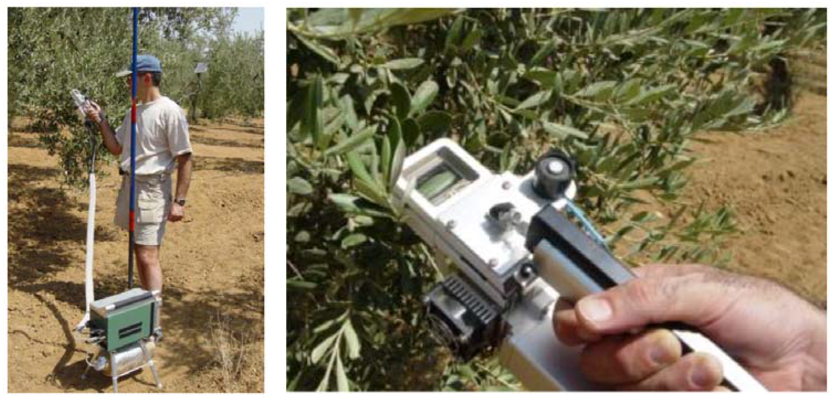
Figure 3.
Scholander chambers for measuring approximate water potential of plant tissue. A model by Soilmoisture Equipment Corp., Santa Barbara, CA (USA), implemented with a binocular stereo microscope and a cold light illuminator (left), and a model by PMS Instrument Company, Albany, OR (USA), implemented with a binocular stereo microscope and a digital manometer (right).
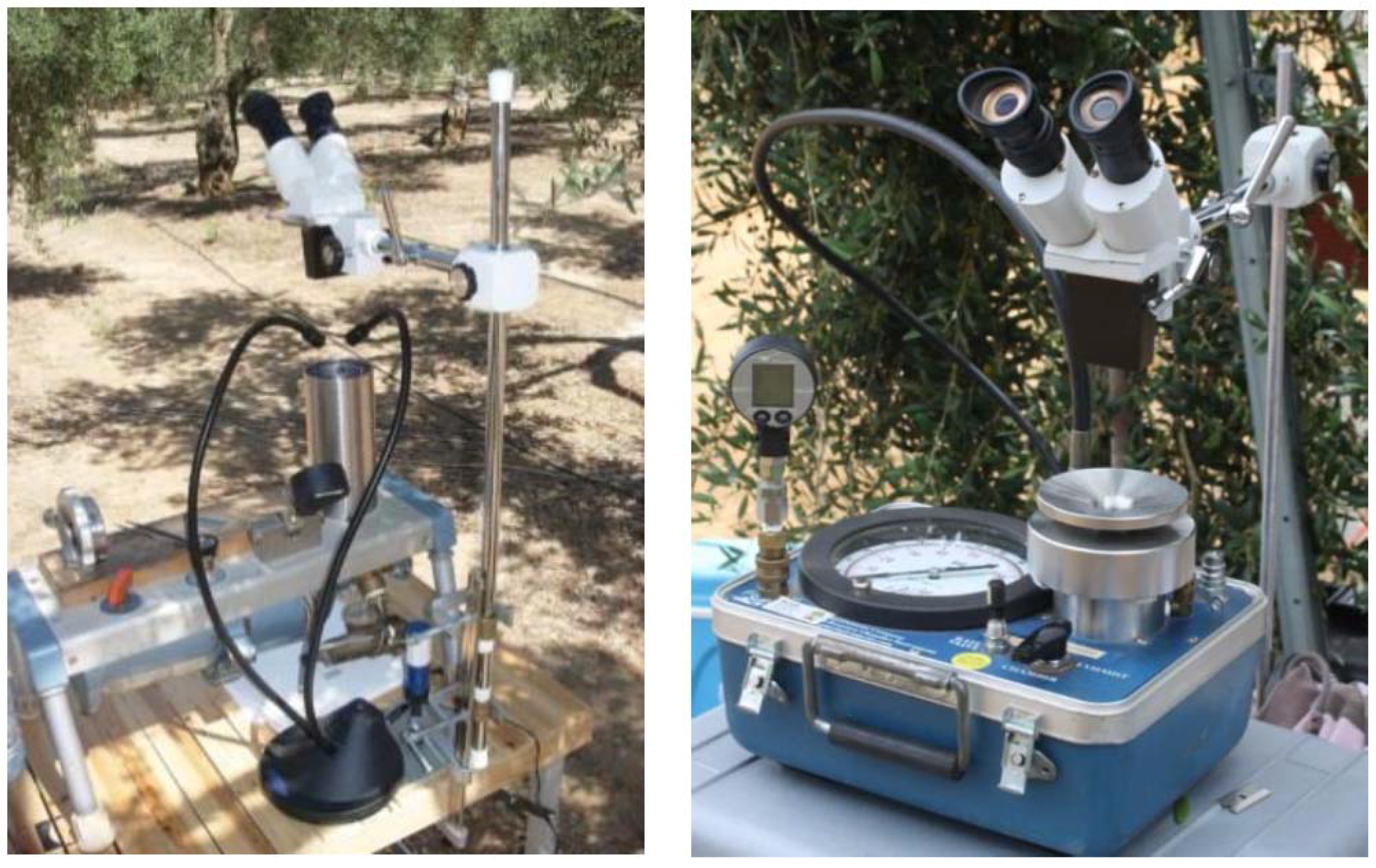
Figure 4.
Diurnal courses of both stomatal conductance (gs) and leaf water potential (Ψl) measured in 39-year-old ‘Manzanilla de Sevilla’ olive trees at 7 m × 5 m spacing in 2007. On 28 August, the first gs measurements are missing because of a problem with the gas analyser. Both for 24 July and 28 August, two clear-sky days of the irrigation season, measurements were taken in trees under three water treatments: (1) Dry-farming, with rainfall as the only source of water supply; (2) Pond, in which the trees were irrigated with a grid of pipes with a 2 L h−1 dripper every 0.4 m × 0.4 m. The grid covered a surface of 8 m × 6 m, with the tree in the middle, enough for keeping non-limiting soil water conditions in the whole root zone, all throughout the irrigation season; and (3) Localized, in which trees were irrigated daily to replace the crop evapotranspiration, with a lateral per tree row with five 3 L h−1 drippers per tree, 1 m apart. With this system some roots were left in drying soil. Differences in gs between the Pond and Localized trees were recorded on both days. Values of Ψl, however, showed that the trees of both treatments had similar water status. Mean ± SE, n = 6. No asterisk means no significant differences; **, *** and **** indicate significant differences at p ≤ 0.01, 0.001 and 0.0001, respectively. See Fernández et al. [53] for details.

Figure 5.
Tree transpiration (Ep) determined by Ohm’s law electrical analogue (Equation (1) in the text) in an orchard with 39-year-old ‘Manzanilla de Sevilla’ olive trees at 7 m × 5 m spacing, under two water treatments leading to contrasting soil water conditions. REW = relative extractable water in the soil; Ψs = soil water potential; Ψl = leaf water potential; and K = hydraulic conductivity. See Fernández et al. [53] for details.

Figure 6.
Images corresponding to the work by Egea et al. [65] in which a thermal infrared (TIR) camera (Tau 2 324, FLIR Systems, Inc., Wilsonville, OR, USA) was mounted on a multirotor RPAS (Remote Piloted Aerial System) model Phantom 2 (SZ DJI Technology Co., Ltd., Shenzhen, China) for thermal imagery acquisition in a high hedgerow olive orchard with 1667 trees per ha (left). Several 0.4 m × 0.5 m black plastic panels were used as a hot reference (central). Images were taken at 20 m above ground and at solar noon of two fully irrigated plots (purple and blue colors) and two deficit-irrigated plots (yellow and orange colors) (right).

Figure 7.
System used by the author to measure sap flow in olive trees with the compensation heat pulse method. It consisted of a solar panel and weather-proof boxes for the electronics (upper box) and battery (lower box) (left). Also shown are sap flow probes inserted into the trunk and a main root of olive trees (right).

Figure 8.
Two different systems for the automatic recording and data transmission of trunk diameter variations. The system on the left consists of LVDT (linear variable differential transformer) dendrometers connected to a Campbell CR1000 data logger (Logan, UT, USA). On the right, a Verdtech station with Plantsens radial dendrometers (Verdtech un Nuevo Campo S.A., Lepe, Spain) is shown, along with a C-Probe (AquaSpy, Inc., San Diego, CA, USA) for the measurement of the soil volumetric water content, two Rain-O-Matic tipping-bucket gauges (Pronamic Co. Ltd, Sikeborg, Denmark), one to record the water supplied by the irrigation system and the other for the precipitation amounts; a combined sensor of temperature and humidity of the air (Vaisala Oyj, Helsinki, Finland) and an addWAVEA733GSM remote telemetry unit (Adcaon Telemetry, Klosterneuburg, Austria).

Figure 9.
Installing the ZIM system in the orchard mentioned in Figure 1 and Figure 6, with the help of Ulrich Zimmermann (in the photo on the right). ZIM probes (left) were connected to a radio transmitter (central up), which sent the collected records to a data logger (central down) located in a weather-proof box at the base of a pool with two aerials (right), one for the radio signals and the other for sending the data from the data logger, via GPRS, to a server.
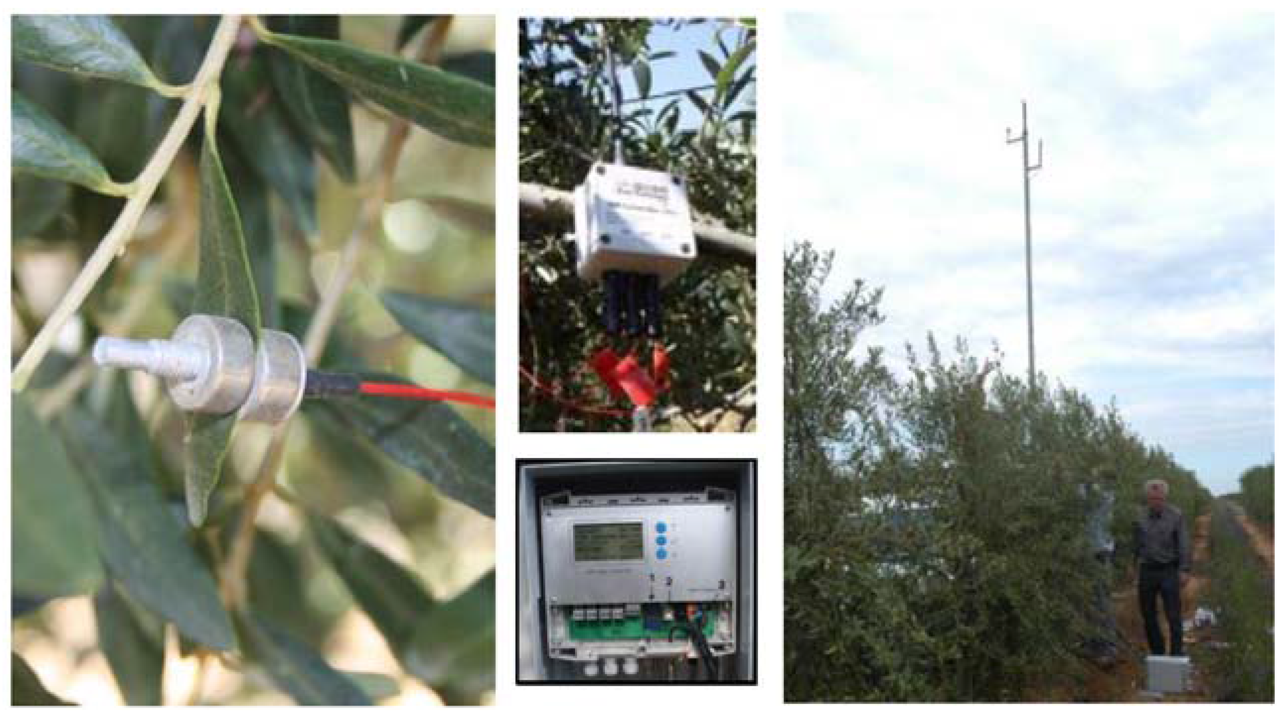
Figure 10.
A TDR probe installed in the trunk of an olive tree for volumetric water content-related measurements (left). The photo was taken during a joint experiment of the author with Dr. Arie Nadler (Institute of Soil, Water, and Environmental Sciences, ARO, Rishon LeZion, Israel), who manufactured the probe. A probe for electric potential-related measurements in the stem of a young fruit-tree (right), manufactured by Dr. Luis Gurovich (Department of Fruit Science, Pontificia Universidad Católica de Chile, Santiago, Chile).
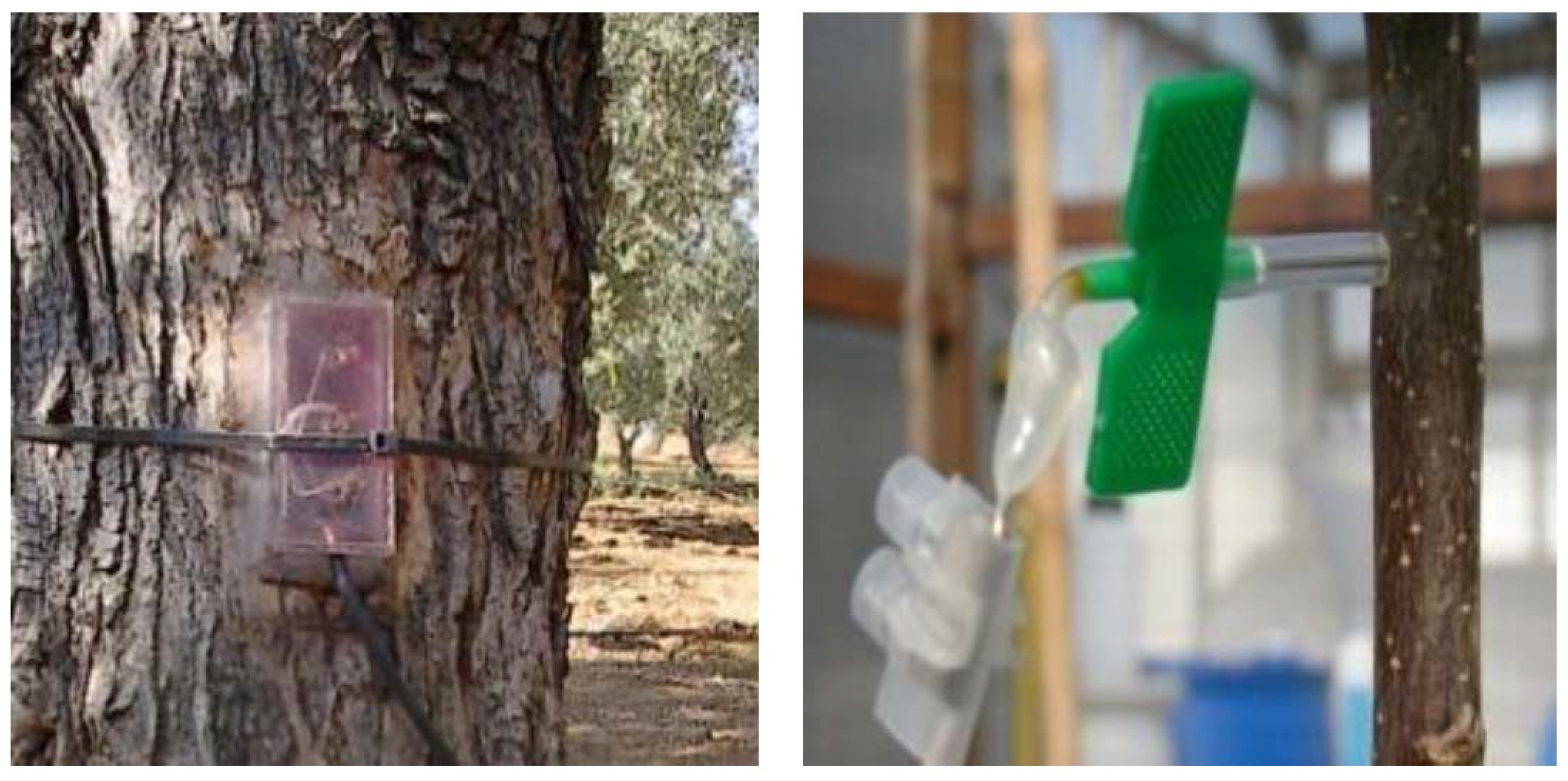

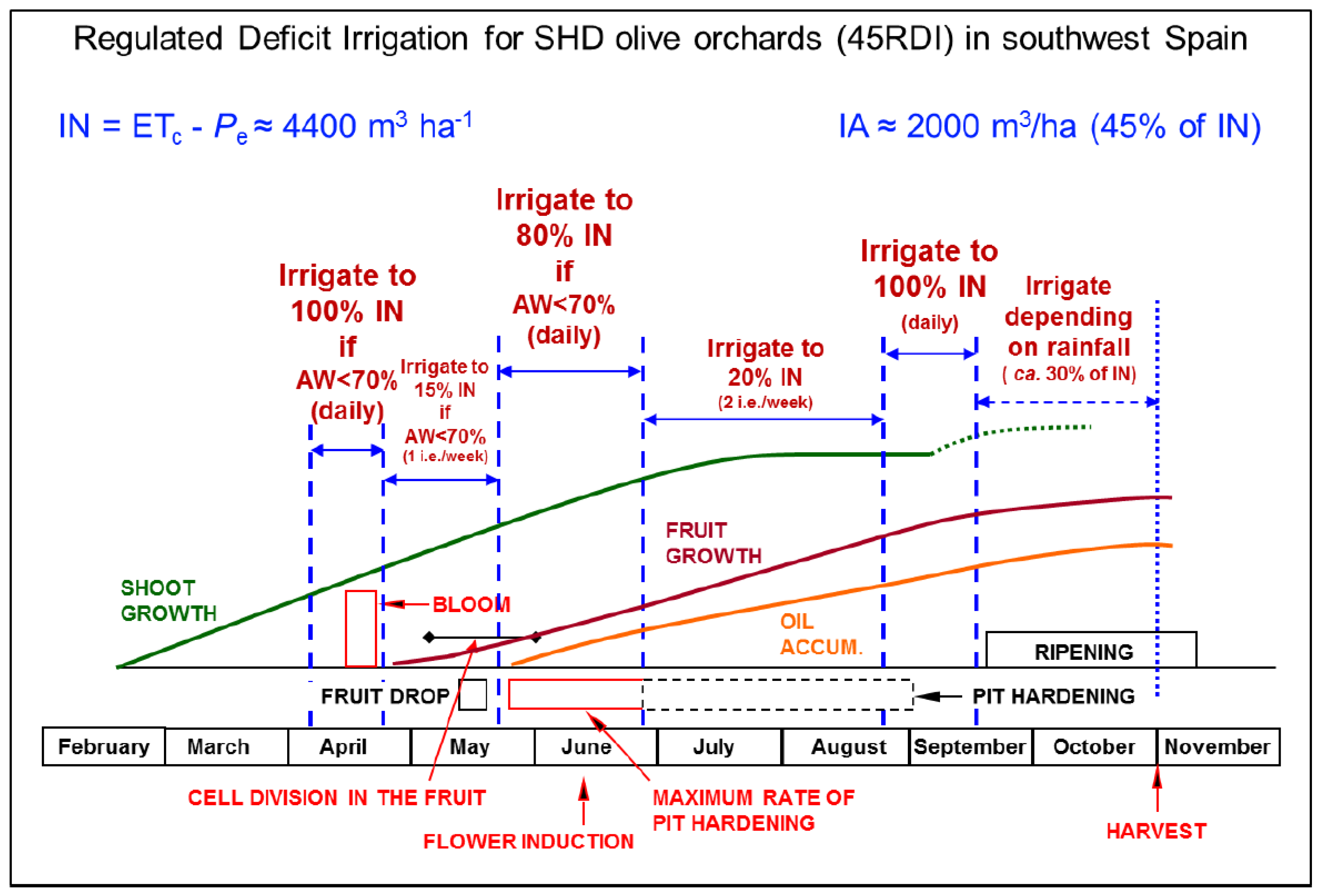
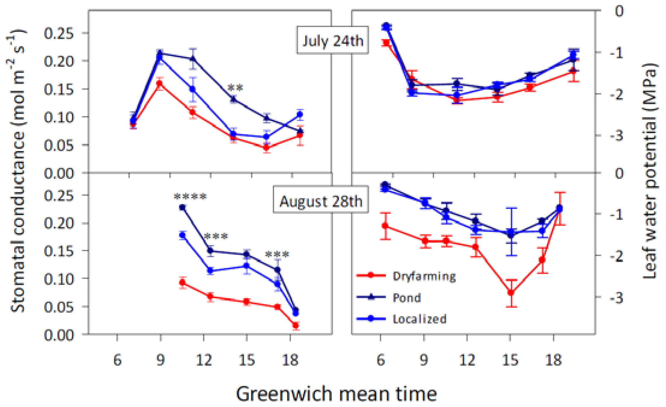
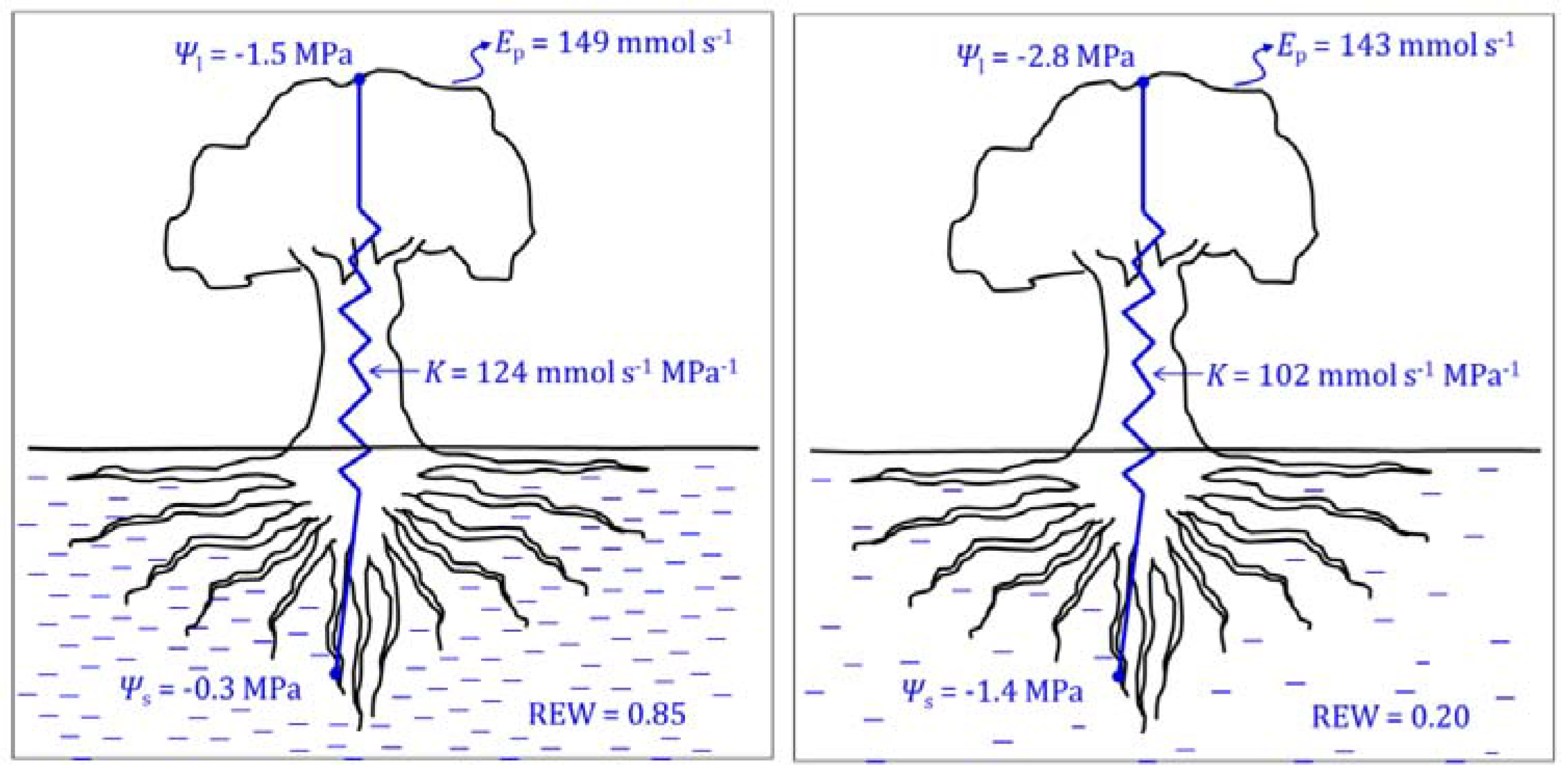
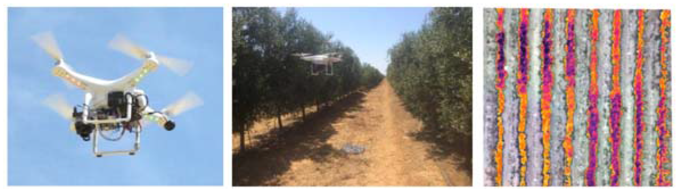
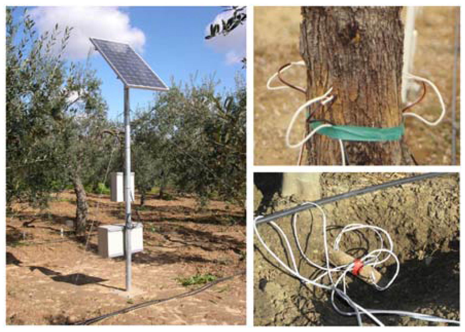
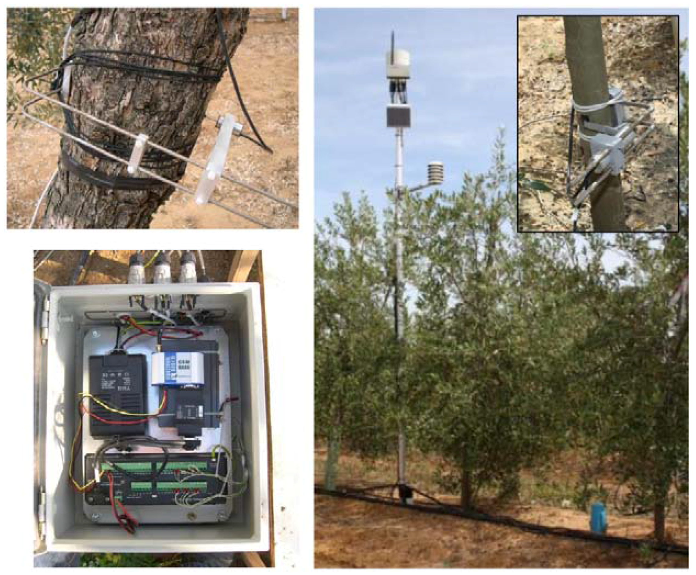
Table 1.
Name, brief definition and key reference papers of the most-used deficit irrigation strategies.
Table 1.
Name, brief definition and key reference papers of the most-used deficit irrigation strategies.
| Strategy | Definition and Remarks | Reference Paper |
|---|---|---|
| Supplementary or complementary irrigation | A single irrigation event is applied when a fixed threshold for water stress is achieved. Just 2 or 3 irrigation events in the irrigation season. Used when water for irrigation is very scarce or in temperate regions with low evapotranspiration rates or high rainfall. It can lead to substantial increases in crop performance, as compared to dry-farming, if the irrigation events are applied at the right moments of the growing cycle. | Abd-Eel-Rahman and El-Sharkawi [8]; Lavee et al. [9]; Proietti et al. [10] |
| Low frequency deficit irrigation (LFDI) | The soil is left to dry until the readily available water is consumed. Irrigation is then applied, until field capacity. This is repeated several times along the irrigation season. | Lavee and Wodner [11] |
| Sustained deficit irrigation (SDI) | A fixed fraction of the crop water needs is applied all throughout the irrigation season. Irrigation is applied daily or 2–4 times per week. | Goldhamer et al. [12]; Grattan et al. [13]; Ramos and Santos [14] |
| Partial root zone drying (PRD) | Similar to SDI, but water is applied to half of the root zone, switching to the other half every 2–3 weeks. | Dry et al. [15]; Fernández et al. [16] |
| Regulated deficit irrigation (RDI) | Irrigation amounts equal or close to the crop water needs are supplied at the phenological stages most sensitive to drought. Irrigation in those periods is applied daily, or at least several times per week. For the rest of the crop cycle, irrigation is drastically reduced (not only the dose is reduced but also the frequency, to one or two irrigation events per week) or even withheld. | Chalmers et al. [17]; Goldhamer [18]; Fernández et al. [6] |
Table 2.
Most-used plant-based measurements and related water stress indicators for irrigation scheduling.
Table 2.
Most-used plant-based measurements and related water stress indicators for irrigation scheduling.
| Measurements Related To | Water Stress Indicator | Symbol or Abbreviation | Units | Remarks |
|---|---|---|---|---|
| Leaf ↔ air gas exchange | Stomatal conductance | gs | mol m−2 s−1 | Recorded with a porometer or an IRGA in plants with waterproof cuticles. |
| gsmax | mol m−2 s−1 | Maximum stomatal conductance, i.e., gs values at the time of maximum stomatal opening. | ||
| Leaf conductance | gl | mol m−2 s−1 | Recorded with a porometer or an IRGA in plants with leaf cuticles permeable to water. | |
| glmax | mol m−2 s−1 | Maximum leaf conductance, i.e., gl values at the time of maximum stomatal opening. | ||
| Net CO2 assimilation or net photosynthesis | A, PN | µmol m−2 s−1 | Net amount of CO2 assimilated per square meter of leaf and per second at the time of the measurement. | |
| Plant water status | Predawn water potential | Ψpd | MPa | |
| Leaf water potential | Ψl | MPa | ||
| Midday leaf water potential | Midday Ψl | MPa | Ψl measured at the time of the day when minimum values are recorded. | |
| Stem water potential | Ψstem | MPa | ||
| Midday stem water potential | Midday Ψstem | MPa | Ψstem measured at the time of the day when minimum values are recorded. | |
| Xylem water potential | Ψx | MPa | Water potential of a branch or trunk, measured with Scholander-type chambers or with microtensiometers. | |
| Balancing pressure | Pb | MPa | Name given by Zimmerman et al. [23] to the output of plant water potential measured with a Scholander-type chamber. | |
| Canopy temperature | Canopy temperature | Tc | °C | |
| Temperature difference between the canopy and the surrounding air | ΔTcanopy-air, Tc − Ta | °C | ||
| Crop water stress index | CWSI | - | Idso et al. [24] stated that its value ranges from 0 (no water stress) to 1 (maximum water stress). | |
| NIR spectroscopy | Estimated Ψl or Ψstem | Ψl or Ψstem | MPa | Leaf or canopy spectral measurements are correlated with values of Ψl or Ψstem made with a Scholander-type chamber, to derive an observed Ψ vs. predicted Ψ relationship. |
| Sap flow | Sap flux density | Jp or Jv | m3 m−2 s−1 | “Flow” points to matter, heat or momentum that is in motion. “Flux” expresses the amount of a substance passing through a given surface per unit of time. “Flux density” is the flux per unit of surface. |
| Sap flux | Qp | m3 s−1 | Total sap flux per plant. Often assumed as equal to total plant transpiration (Ep). | |
| Stem diameter | Maximum daily stem diameter | MXSD | µm | |
| Minimum daily stem diameter | MNSD | µm | ||
| Maximum daily shrinkage | MDS | µm | Difference between the MXSD and the MNSD measured on the day. | |
| Daily recovery | DR | µm | Difference between the MXSD measured on a day and the MNSD measured on the previous day. | |
| Daily growth | DG | µm | Difference between the MXSD measured on a day and the MXSD measured on the previous day. | |
| Stem growth rate | SGR | µm | Average DG for n days. The value of n usually ranges from 3 to 6. | |
| Cumulative growth | CG | µm | The summatory of DG for n days. | |
| Early daily shrinkage | EDS | µm | Stem shrinkage measured between 09.00 and 12.00 hours solar time. | |
| Fruit diameter | Fruit diameter | D | mm | |
| Leaf thickness | Leaf thickness | LT | µm | |
| Leaf turgor pressure | Leaf turgor pressure | Pc | kPa | |
| Pressure signal | Pp | kPa | The output pressure signal provided by the LPCP probe. | |
| Stem water content | Volumetric stem water content | θstem | cm3 cm−3 | Derived from measurements with the TDR method. |
| Stem electrical conductivity | σstem | mS m−1 | Derived from measurements with the TDR method. | |
| Electrical potential | Voltage difference between the leaf zone and the base of the stem | ΔVL-S | mV | |
| Electrical potential | EP | mV | ||
| Relative intensity of the signal | ϕex | % | ||
| Recovery time signal | τ | S |
Table 3.
Characteristics that must be analysed to assess the suitability of any water stress indicator for irrigation scheduling (see Fernández and Cuevas [113] for details).
Table 3.
Characteristics that must be analysed to assess the suitability of any water stress indicator for irrigation scheduling (see Fernández and Cuevas [113] for details).
| Characteristic | Definition | Remarks |
|---|---|---|
| Variability or noise | Accounts for the plant-to-plant variability | Quantified by the coefficient of variation (CV). It must be considered relative to the signal strength. It may increase with water stress. |
| Signal strength or signal intensity, also called signal value or just signal | Signal intensity = actual WSI value/reference WSI value | A high signal value means that the water stress indicator (WSI) responds intensively even to mild water deficits. If the signal strength is sufficient, the noise caused by a high tree-to-tree variability may not be as critical. The actual WSI value is that derived from records made in representative plants, usually under deficit irrigation. See Fernández and Cuevas [113] for details on different approaches to obtain the reference WSI value. |
| Sensitivity, or the signal:noise ratio | Sensitivity = signal intensity/CV | The sensitivity can be calculated if the WSI is based on absolute data, but not when values are relative. See Fernández and Cuevas [113] for alternatives. |
| Earliness | Response of the WSI to the onset of water stress | The WSI responds early to water stress if high signal intensity values are recorded soon after the onset of plant water stress. |
| Reliability | Accounts for the capacity of the sensor and related equipment to perform their required functions under stated conditions for a specified period of time. | All the methods mentioned in Section 2.2 yield reliable WSI. |
| Robustness | Accounts for the capacity of the sensor and related equipment to cope with variations in their operating environment with minimal damage, alteration, or loss of functionality. | All the sensors and related systems mentioned in Section 2.2 are able to work under field conditions for large periods of time. |
Table 4.
Requirements for sensors and related equipment (the system), and for the water stress indicator derived from the collected records, to be used for irrigation scheduling in commercial orchards. After Fernández [20].
Table 4.
Requirements for sensors and related equipment (the system), and for the water stress indicator derived from the collected records, to be used for irrigation scheduling in commercial orchards. After Fernández [20].
| The system must be inexpensive and easy to install, operate and maintain. |
| The system must be reliable and robust, capable of working under field conditions for the whole irrigation season. |
| The system must allow for both automated and continuous collection of clean data and data transmission, i.e., it must be suitable for working properly in electromagnetic-polluted environments and in areas with low cover for data transmission. |
| The system must have low power requirements (e.g., batteries fed with solar panels). |
| The water stress indicator derived from the collected records must be highly sensitive, i.e., it must show a high signal: noise ratio. |
| The indicator must also show an early response to the onset of water stress. |
| The indicator must be related to a variable of economic importance, such as crop yield or fruit quality. |
| The indicator, or the raw sensor outputs in case they are used without any further data processing, must be easy to interpret. |
| If the indicator or raw outputs are not easy to interpret, the system must be provided with an application for visual readouts, graphs, historical records, and other tools to facilitate data interpretation. |
| The system should be easily implemented with an application for the combined use of the chosen indicator with a weather prediction system. This will improve the user capacity for adjusting the timing and intensity of irrigation under changing weather conditions. |
| The system should be easily combined with methods to define areas with characteristic water-stress behaviour within the orchard, such as airborne imagery. This allows for precise irrigation in large, highly variable orchards. |
| The indicator must be suitable for automatic irrigation scheduling and control. In this case, the system should be suitable to be implemented with expert systems, alarms, and other tools for an early detection and lower impact of malfunctions. |
© 2017 by the author. Licensee MDPI, Basel, Switzerland. This article is an open access article distributed under the terms and conditions of the Creative Commons Attribution (CC BY) license (http://creativecommons.org/licenses/by/4.0/).
Share and Cite
MDPI and ACS Style
Fernández, J.E. Plant-Based Methods for Irrigation Scheduling of Woody Crops. Horticulturae 2017, 3, 35. https://doi.org/10.3390/horticulturae3020035
AMA Style
Fernández JE. Plant-Based Methods for Irrigation Scheduling of Woody Crops. Horticulturae. 2017; 3(2):35. https://doi.org/10.3390/horticulturae3020035
Chicago/Turabian StyleFernández, José Enrique. 2017. "Plant-Based Methods for Irrigation Scheduling of Woody Crops" Horticulturae 3, no. 2: 35. https://doi.org/10.3390/horticulturae3020035
Note that from the first issue of 2016, this journal uses article numbers instead of page numbers. See further details here.