
LaFiDa—A Laserscanner Multi-Fisheye Camera Dataset


Institute of Photogrammetry and Remote Sensing (IPF) Karlsruhe Institute of Technology (KIT), Englerstr. 7, 76131 Karlsruhe, Germany
*
Authors to whom correspondence should be addressed.
J. Imaging 2017, 3(1), 5; https://doi.org/10.3390/jimaging3010005
Submission received: 22 September 2016
/
Revised: 14 December 2016
/
Accepted: 4 January 2017
/
Published: 17 January 2017
(This article belongs to the Special Issue 3D Imaging)
Abstract
:In this article, the Laserscanner Multi-Fisheye Camera Dataset (LaFiDa) for applying benchmarks is presented. A head-mounted multi-fisheye camera system combined with a mobile laserscanner was utilized to capture the benchmark datasets. Besides this, accurate six degrees of freedom (6 DoF) ground truth poses were obtained from a motion capture system with a sampling rate of 360 Hz. Multiple sequences were recorded in an indoor and outdoor environment, comprising different motion characteristics, lighting conditions, and scene dynamics. The provided sequences consist of images from three—by hardware trigger—fully synchronized fisheye cameras combined with a mobile laserscanner on the same platform. In total, six trajectories are provided. Each trajectory also comprises intrinsic and extrinsic calibration parameters and related measurements for all sensors. Furthermore, we generalize the most common toolbox for an extrinsic laserscanner to camera calibration to work with arbitrary central cameras, such as omnidirectional or fisheye projections. The benchmark dataset is available online released under the Creative Commons Attributions Licence (CC-BY 4.0), and it contains raw sensor data and specifications like timestamps, calibration, and evaluation scripts. The provided dataset can be used for multi-fisheye camera and/or laserscanner simultaneous localization and mapping (SLAM).
1. Introduction
Benchmark datasets are essential for the evaluation and objective assessment of the quality, robustness, and accuracy of methods developed in research. In this article, the Laserscanner Multi-Fisheye Camera Dataset LaFiDa (the acronym LaFiDa is based on the Italian term “la fida”, which stands for trust/faithful) with accurate six degrees of freedom (DoF) ground truth for a head-mounted multi-sensor system is presented. The dataset is provided to support objective research; e.g., for applications like multi-sensor calibration and multi-camera simultaneous localization and mapping (SLAM). Especially, methods developed for challenging indoor and outdoor scenarios with difficult illumination conditions, narrow and obstructed paths, and moving objects can evaluated. Multiple sequences are recorded in an indoor and outdoor (Figure 1b) environment, and comprise sensor readings from a laserscanner and three fisheye cameras mounted on a helmet. Apart from the raw timestamped sensor data, we provide the scripts and measurements to calibrate the intrinsic and extrinsic parameters of all sensors, making the immediate use of the dataset easier. Still, all raw calibration data is contained in the dataset to assess the impact of new calibration methodologies (e.g., different camera models) on egomotion estimation.
The article is organized as follows. After briefly discussing related work in Section 2, we introduce the utilized sensors and the mounting setup on the helmet system in Section 3. In Section 4, the extensive procedure with all methods for the determination of the intrinsic parameters of each fisheye camera and the corresponding extrinsic parameters (relative orientations) between all sensors is described. After presenting the specifications of the indoor and outdoor datasets with the six trajectories in Section 5, the concluding remarks and suggestions for future work are finally provided in Section 6.
2. Related Work
Many datasets for the evaluation of visual odometry (VO) and SLAM methods exist, and are related to this work and subsumed in Table 1. However, this section is far from exhaustive, and we focus on the most common datasets. Accurate ground truth from a motion capture system for a single RGB-D camera (“D” refers to “depth” or “distance”) is presented in the TUM RGB-D dataset [1]. In [2], the authors present a complete overview of RGB-D datasets not only for VO, but also object pose estimation, tracking, segmentation, and scene reconstruction.
In [3], the authors additionally provide photometric calibrations for 50 sequences of a wide-angle and a single fisheye camera for monocular SLAM evaluation. The KITTI dataset [4] comes with multiple stereo datasets from a driving car with GPS/INS ground truth for each frame. In [5], ground truth poses from a lasertracker as well as a motion capture system for a micro aerial vehicle (MAV) are presented. The dataset contains all sensor calibration data and measurements. In addition, 3D laser scans of the environment are included to enable the evaluation of reconstruction methods. The MAV is equipped with a stereo camera and an inertial measurement unit (IMU).
For small-to-medium scale applications, certain laser- and camera-based datasets are provided by Rawseeds [6]. They contain raw sensor readings from IMUs, a laserscanner, and different cameras mounted onto a self-driving multi-sensor platform. Aiming at large scale applications, the Malaga datasets [7] contain centimeter-accurate Global Positioning System (GPS) ground truth for stereo cameras and different laserscanners. The New College dataset [8] includes images from of a platform driving around the campus. Several kilometers are covered, but no accurate ground truth is available.
From this review of related datasets, we can identify our contributions and the novelty of this article:
- Acquisition platform and motion: Most datasets are either acquired from a driving sensor platform [4,6,7,8] or hand-held [1,3]. Either way, the datasets have distinct motion characteristics—especially in the case of vehicles. Our dataset is recorded from a head-mounted sensor platform, introducing different viewpoint and motion characteristics from a pedestrian.
- Environment model: In addition, we include a dense 3D model of the environment to enable new types of evaluation; e.g., registering SLAM trajectories to 3D models or comparing laserscanner to image-based reconstructions.
3. Sensors and Setup
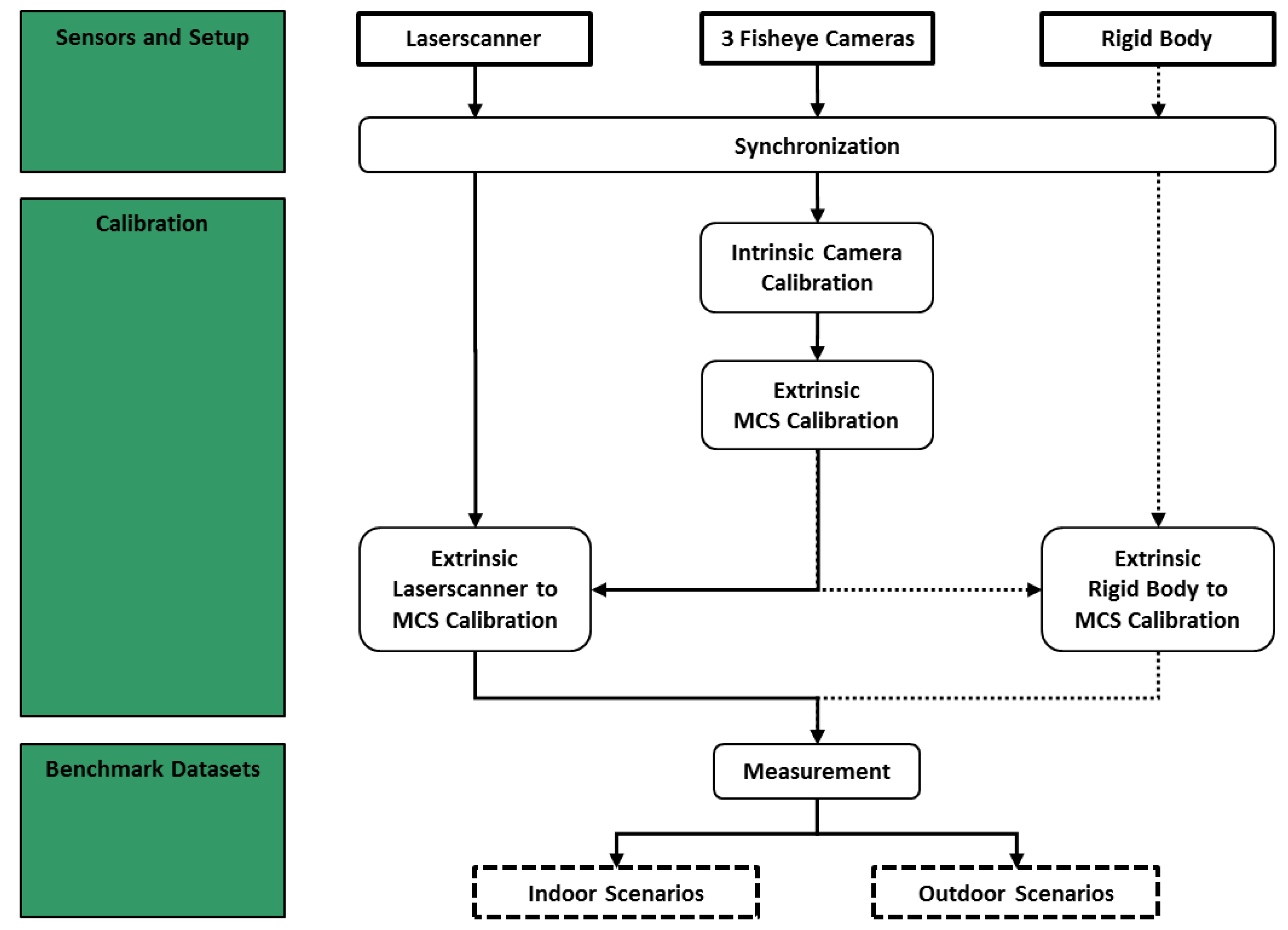
In this section, the sensors and their setup on the helmet system are presented. A general overview of the workflow is depicted in Figure 2. In addition, information about the motion capture system that is used to acquire the ground truth is given. Table 2 provides a brief overview of the specifications of all sensors. Further information can be found on the corresponding manufacturer websites.
3.1. Laserscanner
To obtain accurate 3D measurements and make mapping and tracking in untextured environments with difficult lighting conditions possible, a Hokuyo (Osaka, Japan) UTM-30LX-EW laserscanner was used. Typical applications might include supporting camera-based SLAM or laserscanner-only mapping. According to the specifications, this device emits laser pulses with a wavelength of λ = 905 nm, and the laser safety is class 1. It has an angular resolution of 0.25° and measures with a field of view (FoV) of 270°. The distance accuracy is specified with ±30 mm between 0.1 m and 10 m distance. The maximum measurement distance is 30 m. The specified pulse repetition rate is 43 kHz (i.e., 40 scan lines (40 Hz) are captured per second). With its size of 62 mm × 62 mm × 87.5 mm and a weight of 210 g (without cable), the laserscanner is well suited for building up a compact helmet system.
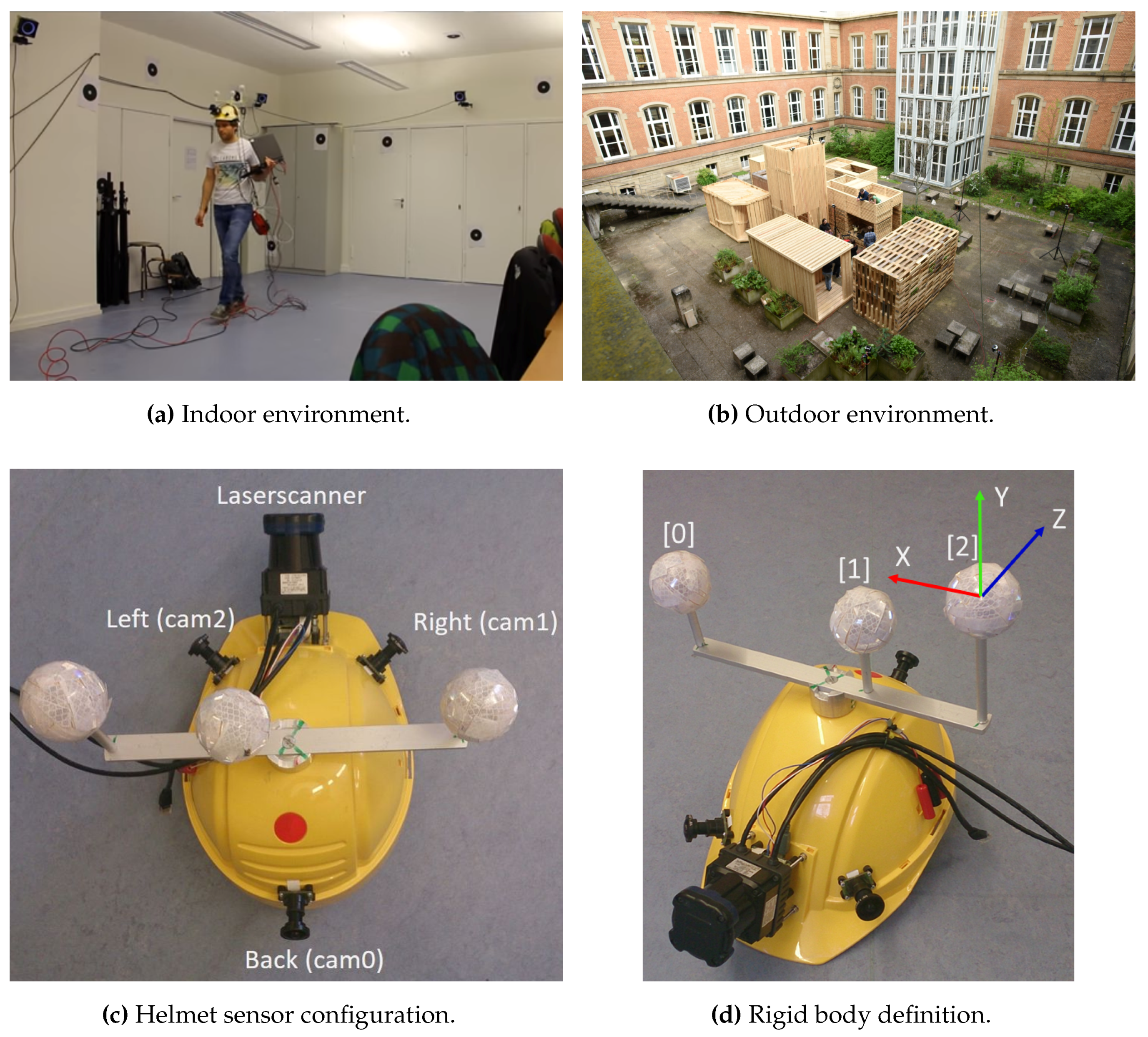
The laserscanner is mounted to the front of the helmet in an oblique angle (see Figure 1c), scanning the ground ahead of and next to the operator. The blind spot of 90° is in the upward direction, which is feasible, especially outdoors. For each scan line, we record a timestamp, the distances, and scan angle of each laser pulse, as well as its intensity value. The laserscanner is connected to the laptop with a USB3.0-to-Gbit LAN adapter.
3.2. Multi-Fisheye Camera System
The Multi-Fisheye Camera System (MCS) consists of a multi-sensor USB platform from VRmagic (VRmC-12) with an integrated field programmable gate array (FPGA). Hardware-triggered image acquisition and image pre-processing is handled by the platform, and thus all images are captured pixel synchronous. We connected three CMOS (Complementary Metal Oxide Semiconductor) camera sensors with a resolution of 754 × 480 pixels to the platform running with 25 Hz sampling rate. The sensors were equipped with similar fisheye lenses from Lensagon (BF2M12520) having a FoV of approximately 185° and a focal length of 1.25 mm. The USB platform was connected to the laptop via USB 2.0. To provide examples of the captured data a set of three fisheye images acquired indoor and outdoor respectively is depicted in Figure 3.
3.3. Rigid Body
To acquire accurate 6 DoF ground truth for the motion of the multi-sensor helmet system, a motion capture system (OptiTrack (Corvallis, OR, USA), Prime 17W) with eight hardware-triggered high-speed cameras was used. The system needs to be calibrated in advance by waving a calibration stick with three passive spherical retro-reflective markers in the volume that the cameras observe. As the exact metric dimension of the calibration stick is known, the poses of all motion capture cameras can be recovered metrically.
Once the motion capture system is calibrated, the 3 DoF position of markers can be tracked by triangulation with 360 Hz and sub-millimeter accuracy. To determine the 6 DoF motion of our helmet system, at least three markers are necessary to create a distinct coordinate frame. The combination of multiple markers is called a rigid body, and the rigid body definition of our system is depicted in Figure 1d. As the tracking system might lose the position of the markers from time to time, we verify the distinct number of each marker that is used to define the rigid body coordinate frame by comparing the mutual distances. The marker positions are broadcasted over Ethernet, and the rigid body is created on-the-fly with each broadcasted marker set.
4. Calibration
We provide ready-to-use calibration data for the intrinsics of each fisheye camera and the extrinsic parameters (relative orientations) between all sensors (Figure 2). Still, the raw calibration data is contained in the dataset to test the impact of different camera models or calibration methods.
In the following, transformation matrices between the different sensors are estimated. In particular, besides the camera intrinsics (cf. Section 4.1), we calibrate the extrinsics between the sensors:
- MCS: The MCS calibration contains the relative MCS frame t to camera c transformations (cf. Section 4.2). The MCS frame can either be coincident with a camera frame or be defined virtually (e.g., in the centroid of all cameras).
- Lasercanner to MCS: In this step, the laserscanner is calibrated to a fisheye camera (cam2 in Figure 1c), yielding the transformation matrix: (cf. Section 4.3).
- Rigid body to MCS: Finally, we estimate the rigid body to MCS transformation (cf. Section 4.4).
4.1. Intrinsic Camera Calibration
We use the omnidirectional camera model proposed in [12], and calibrate all involved parameters using an improved version of the original toolbox [13]. Multiple images of a checkerboard were recorded with each camera, and are all available in the dataset. The intrinsics were assumed to be stable over the time for recording different trajectories.
4.2. Extrinsic Multi-Camera System Calibration
The extrinsic multi-camera system calibration is performed from control points which are equally distributed in the motion capture volume. The control points are large black circles whose 3D coordinates are defined by a smaller retro reflective circle placed in the center of the large black circle. The corresponding 2D measurement is obtained by fitting an ellipse to the dark region in the images. The extrinsics of an MCS consist of the MCS frame to camera frame transformations:
where is the rotation and the translation of a camera frame c to the MCS frame. The MCS frame is a virtual frame that is rigidly coupled to the MCS and defines the exterior orientation of the MCS at a certain time t.
In order to calibrate the MCS, we record a set of images with at multiple timesteps from different viewpoints. Subsequently, the following procedure is carried out:
- Select points in each image c at all timesteps t.
- Define MCS pose , by initializing the rotation to the rotation of the first camera (i.e., ) and setting the offset vector to the mean offset from all camera poses .
- Extract all MCS to camera frame transformations .
This procedure separates the exterior orientation of each single camera into two transformations; i.e., the world to MCS and the MCS to camera transformation. The last step of the procedure yields initial values for the MCS to camera frame transformations, but are only averaged over all timesteps. Thus, in a last step, MultiCol [16] is used to simultaneously refine all MCS poses and body to camera transformations .
4.3. Extrinsic Laserscanner to MCS Calibration
Extrinsic calibration can be usually tackled by image-based strategies for the same type of sensors [17], but even for different type of sensors [18]. However, determining the extrinsics between a laserscanner and a pinhole camera is already challenging [9,10,11]. In this article, we extend an algorithm [9] that was developed to calibrate laserscanners to pinhole camera making it now applicable to all types of central cameras, including omnidirectional and fisheye projections.
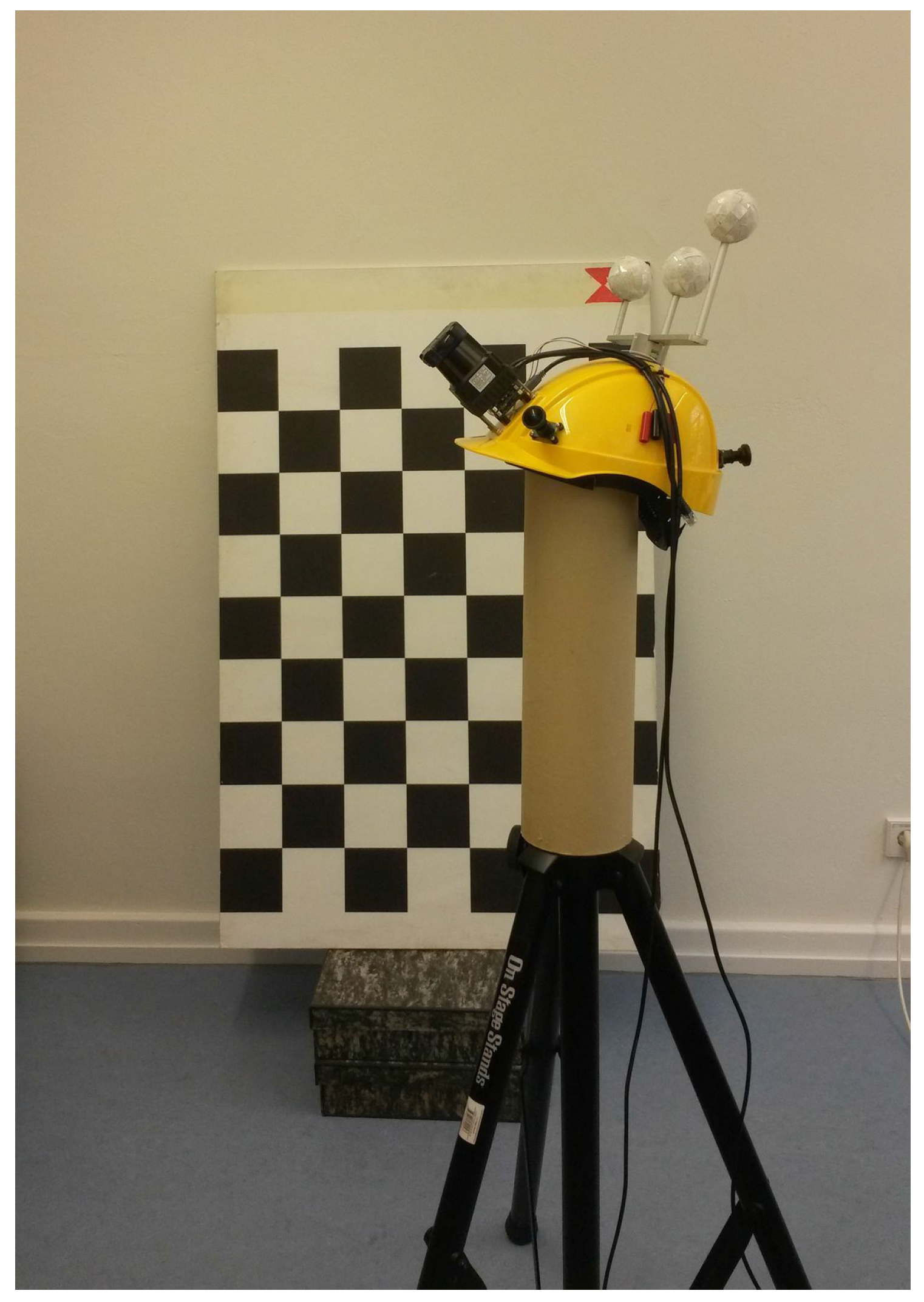
The purpose of this calibration step is to find the transformation matrix that maps laserscanner measurements to one of the fisheye cameras. For practical reasons, we select the fisheye camera which is located on the left side next to the laserscanner (cam2 in Figure 1c). To calibrate the laserscanner to one of the fisheye cameras, a checkerboard is observed multiple times from different viewpoints (depicted in Figure 4). Then, the following processing steps are conducted (the code is also available online):
- Extract checkerboard points from all images.
- Estimate all camera poses using a PnP algorithm w.r.t. the checkerboard frame.
- Improve laserscanner accuracy by averaging over five consecutive measurements for each timestamp. We record multiple scan lines from each viewpoint.
- Estimate the transformation matrix using [20].
An import remark is that the extrinsic calibration is not possible with RADLOCC, as the transformation matrix is initialized with an identity in their implementation [9]. With this specific assumption, the optimization would not converge in our case, as laserscanner and camera frames are heavily tilted w.r.t to each other; i.e., the transformation is far from being an identity. Hence, the minimal and stable solution provided by [20] is used to find .
4.4. Extrinsic Rigid Body to MCS Calibration
In a last calibration step, we estimate the transformation matrix between rigid body and MCS frame. Again, we record a set of images from multiple viewpoints in a volume that contains the control points used during MCS calibration (cf. Section 4.2). Subsequently, we extract the corresponding 2D image measurements with subpixel accuracy. For each viewpoint, we also record the rigid body pose . Now, we can project a control point into the camera images at one timestep t with the following transformation chain:
where is the reprojected control point i at time t in camera c. Finally, we can optimize the relative transformation by minimizing the reprojection error utilizing the Levenberg–Marquardt algorithm.
5. Benchmark Datasets
To be able to test and evaluate methods developed in this article, we record multiple trajectories with different characteristics. Dynamic and static scenes are recorded having different translational and rotational velocities and lengths. In addition, indoor and outdoor scenes are considered covering narrow and wider areas as well as different illumination conditions (Figure 2). The trajectory characteristics are subsumed in Table 3.
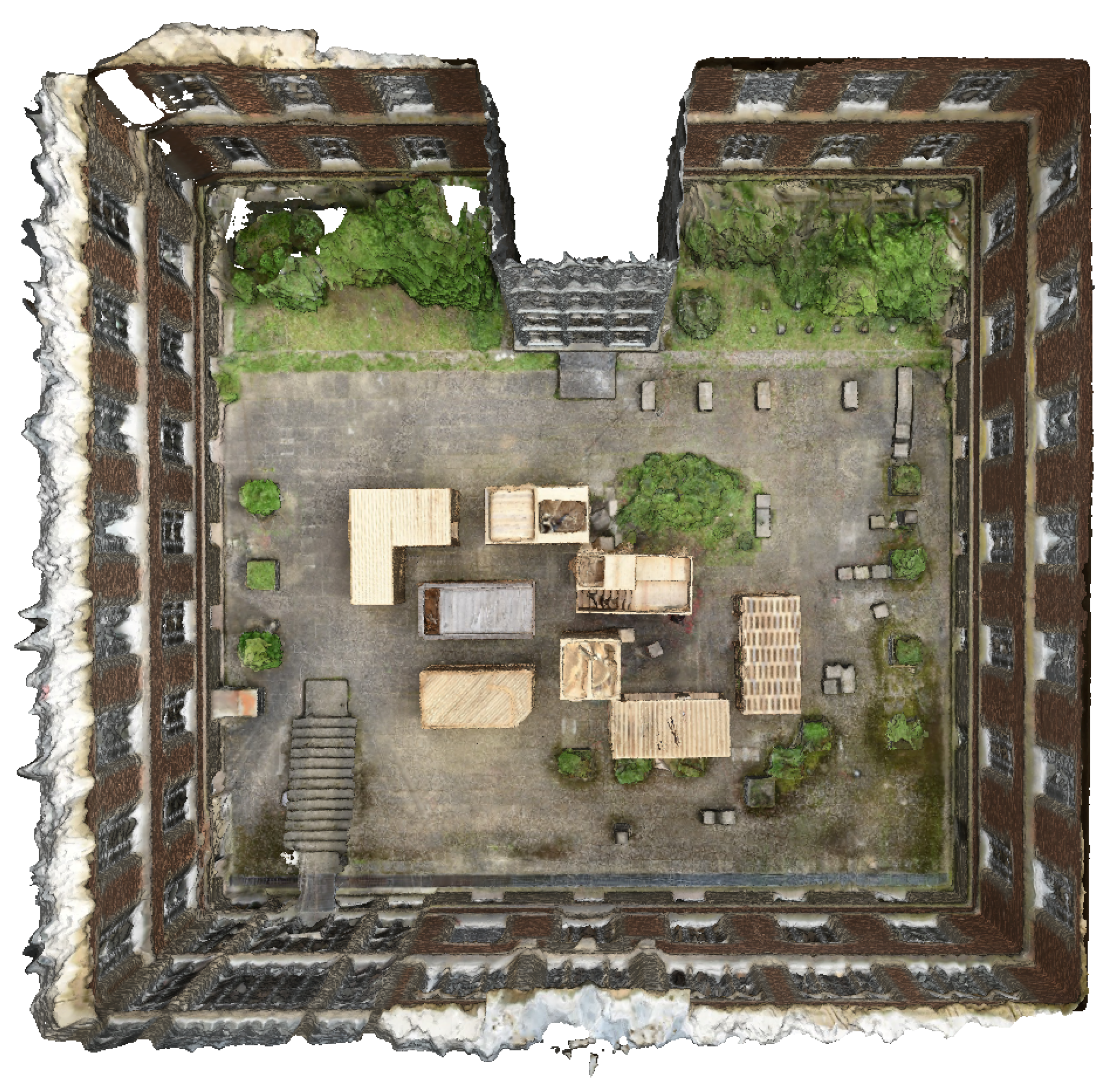
In addition, a textured 3D model of the outdoor scene is created, which can be used for comparison purposes or just to get an impression of the scene. Therefore, more than 500 high-resolution images are utilized. The images are captured using a NIKON (Tokyo, Japan) D810 equipped with a 20 mm fixed focus lens. The CMOS sensor has a resolution of approximately 36 Mpix. For processing the data to derive a textured 3D model, AgiSoft Photocan (St. Petersburg, Russia) software is used. A bird eye view of the 3D model is depicted in Figure 5.
The dataset is available online [21] released under the Creative Commons Attributions Licence (CC-BY 4.0), and it contains raw sensor data and specifications like timestamps, calibration, and evaluation scripts. The complete amount of the provided data is currently about 8 gigabytes.
6. Synchronization
The different types of sensors are triggered in a different manner. The three cameras are hardware triggered by the USB platform, and thus a single timestamp is taken for all images as they are recorded pixel synchronous. More detailed specifications can be found at: [22]. On the other hand, the laserscanner is a continuous scanning device, and an acquisition cannot be hardware triggered—only a timestamp for each scan line can be taken. Due to the different acquisition rates of both senors, only a nearest neighbor timestamp can be taken to get corresponding measurements for both sensors. Assuming a ground truth acquisition rate of 360 Hz, the maximum difference between a ground truth timestamp and a sensor measurement (either camera or laserscanner) is below 1.4 ms.
All sensors as well as the motion capture system are connected to a laptop with an Intel (Santa Clara, CA, USA) Core i7-3630QM CPU. The data is recorded onto a Samsung (Seoul, South Korea) SSD 850 EVO from a single program, and each incoming sensor reading gets timestamped. In this way, we avoid errors that would be introduced by synchronization from different sensors’ clocks. Software synchronization, however, depends on the internal clock of the computer, which can drift. In this work, we did not investigate the errors introduced by inaccurate software timestamps, and leave this open to future work.
7. Known Issues
There exist some known issues in the dataset. These, however, should not affect the usability or the accuracy of the ground truth, which is supposed to be on the order of millimeters. Some of them will be addressed and corrected in future work.
- Clock drift: The internal clocks of MCS, laserscanner, and motion capture system are independent, which might result in a temporal drift of the clocks. However, as the datasets are relatively short (1–4 min), this should not affect the accuracy.
- Equidistant timestamps: All data were recorded to the hard drive during acquisition. This led to some frames being dropped. In addition, auto gain and exposure as well as black level and blooming correction was enabled on the imaging sensor, resulting in a varying frame rate. Still, all images were acquired pixel synchronous, which is guaranteed by the internal hardware trigger of the USB-platform.
8. Conclusions
In this article, an accurate ground truth dataset for a head-mounted multi-sensor system is presented. In future work, we want to integrate larger trajectories into the dataset and add data from the same environment at different times (day, year) to make the evaluation of methods possible for the community that aim at long term tracking, mapping, and re-localization.
Acknowledgments
This project is partially funded by the German Research Foundation (DFG) research group FG 1546 “Computer-Aided Collaborative Subway Track Planning in Multi-Scale 3D City and Building Models”. Further, the authors would like to thank the master students of Geodesy and Geoinformatics at KIT for their support.
Author Contributions
Steffen Urban and Boris Jutzi conceived and designed the experiments, analyzed the data, developed the analysis tools, and wrote the paper.
Conflicts of Interest
The authors declare no conflict of interest.
References
- Sturm, J.; Engelhard, N.; Endres, F.; Burgard, W.; Cremers, D. A Benchmark for the Evaluation of RGB-D SLAM Systems. In Proceedings of the International Conference on Intelligent Robot Systems (IROS), Vilamoura-Algarve, Portugal, 7–12 October 2012.
- Firman, M. RGBD Datasets: Past, Present and Future. 2016. Available online: https://arxiv.org/abs/1604.00999 (accessed on 6 January 2017).
- Engel, J.; Usenko, V.; Cremers, D. A Photometrically Calibrated Benchmark For Monocular Visual Odometry. 2016. Available online: https://arxiv.org/abs/1607.02555 (accessed on 6 January 2017).
- Geiger, A.; Lenz, P.; Stiller, C.; Urtasun, R. Vision meets Robotics: The KITTI Dataset. Int. J. Robot. Res. (IJRR) 2013, 32, 1231–1237. [Google Scholar] [CrossRef]
- Burri, M.; Nikolic, J.; Gohl, P.; Schneider, T.; Rehder, J.; Omari, S.; Achtelik, M.W.; Siegwart, R. The EuRoC Micro Aerial Vehicle Datasets. Int. J. Robot. Res. 2016, 35, 1157–1163. [Google Scholar] [CrossRef]
- Ceriani, S.; Fontana, G.; Giusti, A.; Marzorati, D.; Matteucci, M.; Migliore, D.; Rizzi, D.; Sorrenti, D.G.; Taddei, P. Rawseeds Ground Truth Collection Systems for Indoor Self-Localization and Mapping. Auton. Robot. 2009, 27, 353–371. [Google Scholar] [CrossRef]
- Blanco, J.L.; Moreno, F.A.; Gonzalez, J. A collection of outdoor robotic datasets with centimeter-accuracy ground truth. Auton. Robot. 2009, 27, 327–351. [Google Scholar] [CrossRef]
- Smith, M.; Baldwin, I.; Churchill, W.; Paul, R.; Newman, P. The new college vision and laser data set. Int. J. Robot. Res. (IJRR) 2009, 28, 595–599. [Google Scholar] [CrossRef]
- Zhang, Q.; Pless, R. Extrinsic Calibration of a Camera and Laser Range Finder (Improves Camera Calibration). In Proceedings of the IEEE/RSJ Conference on Intelligent Robots and Systems (IROS), Sendai, Japan, 28 September–2 October 2004.
- Jutzi, B.; Weinmann, M.; Meidow, J. Weighted data fusion for UAV-borne 3D mapping with camera and line laser scanner. Int. J. Image Data Fusion 2014, 5, 226–243. [Google Scholar] [CrossRef]
- Atman, J.; Popp, M.; Ruppelt, J.; Trommer, G.F. Navigation Aiding by a Hybrid Laser-Camera Motion Estimator for Micro Aerial Vehicles. Sensors 2016, 16, 1516. [Google Scholar] [CrossRef] [PubMed]
- Scaramuzza, D.; Martinelli, A.; Siegwart, R. A flexible technique for accurate omnidirectional camera calibration and structure from motion. In Proceedings of the Fourth IEEE International Conference on Computer Vision Systems (ICVS), New York, NY, USA, 4–7 January 2006.
- Urban, S.; Leitloff, J.; Hinz, S. Improved wide-angle, fisheye and omnidirectional camera calibration. ISPRS J. Photogramm. Remote Sens. 2015, 108, 72–79. [Google Scholar] [CrossRef]
- Urban, S.; Leitloff, J.; Hinz, S. MLPnP: A Real-Time Maximum Likelihood Solution to the Perspectinve-N-Point problem. ISPRS Ann. Photogramm. Remote Sens. Spat. Inf. Sci. 2016, 3, 131–138. [Google Scholar] [CrossRef]
- Zheng, Y.; Kuang, Y.; Sugimoto, S.; Astrom, K.; Okutomi, M. Revisiting the PnP problem: A fast, general and optimal solution. In Proceedings of the International Conference on Computer Vision (ICCV), Sydney, Australia, 1–8 December 2013.
- Urban, S.; Wursthorn, S.; Leitloff, J.; Hinz, S. MultiCol Bundle Adjustment: A Generic Method for Pose Estimation, Simultaneous Self-Calibration and Reconstruction for Arbitrary Multi-Camera Systems. Int. J. Comput. Vision (IJCV) 2016, 1–19. [Google Scholar] [CrossRef]
- Weinmann, M.; Jutzi, B. Fully automatic image-based registration of unorganized TLS data. Int. Arch. Photogramm. Remote Sens. Spat. Inf. Sci. 2011, XXXVIII-5/W12, 55–60. [Google Scholar] [CrossRef]
- Weinmann, M.; Hoegner, L.; Leitloff, J.; Stilla, U.; Hinz, S.; Jutzi, B. Fusing passive and active sensed images to gain infrared-textured 3D models. Int. Arch. Photogramm. Remote Sens. Spat. Inf. Sci. 2012, XXXIX-B1, 71–76. [Google Scholar] [CrossRef]
- Kassir, A.; Peynot, T. Reliable Automatic Camera-Laser Calibration. In Proceedings of the 2010 Australasian Conference on Robotics & Automation (ARAA), Brisbane, Australia, 1–3 December 2010.
- Vasconcelos, F.; Barreto, J.P.; Nunes, U. A Minimal Solution for the Extrinsic Calibration of a Camera and a Laser-Rangefinder. IEEE Trans. Pattern Anal. Mach. Intell. (PAMI) 2012, 34, 2097–2107. [Google Scholar] [CrossRef] [PubMed]
- LaFiDa - A Laserscanner Multi-Fisheye Camera Dataset. 2017. Available online: https://www.ipf.kit.edu/lafida.php (accessed on 6 January 2017).
- VRmagic VRmC-12/BW OEM (USB-Platform). 2016. Available online: https://www.vrmagic.com/fileadmin/downloads/imaging/Camera_Datasheets/usb_cameras/VRmMFC_multisensor.pdf (accessed on 6 January 2017).
Figure 1.
Depicted are the (a) indoor and (b) outdoor scenes. In (c,d) the helmet sensor configuration and the rigid body definition (colored coordinate frame) are pictured. The three reflective rigid body markers (spheres) are enumerated with [0],[1],[2].
Figure 1.
Depicted are the (a) indoor and (b) outdoor scenes. In (c,d) the helmet sensor configuration and the rigid body definition (colored coordinate frame) are pictured. The three reflective rigid body markers (spheres) are enumerated with [0],[1],[2].

Figure 2.
Workflow of the Laserscanner Multi-Fisheye Camera Dataset (LaFiDa). MCS: multi-fisheye camera system.
Figure 2.
Workflow of the Laserscanner Multi-Fisheye Camera Dataset (LaFiDa). MCS: multi-fisheye camera system.

Figure 3.
Set of three fisheye images acquired (a) indoors and (b) outdoors.
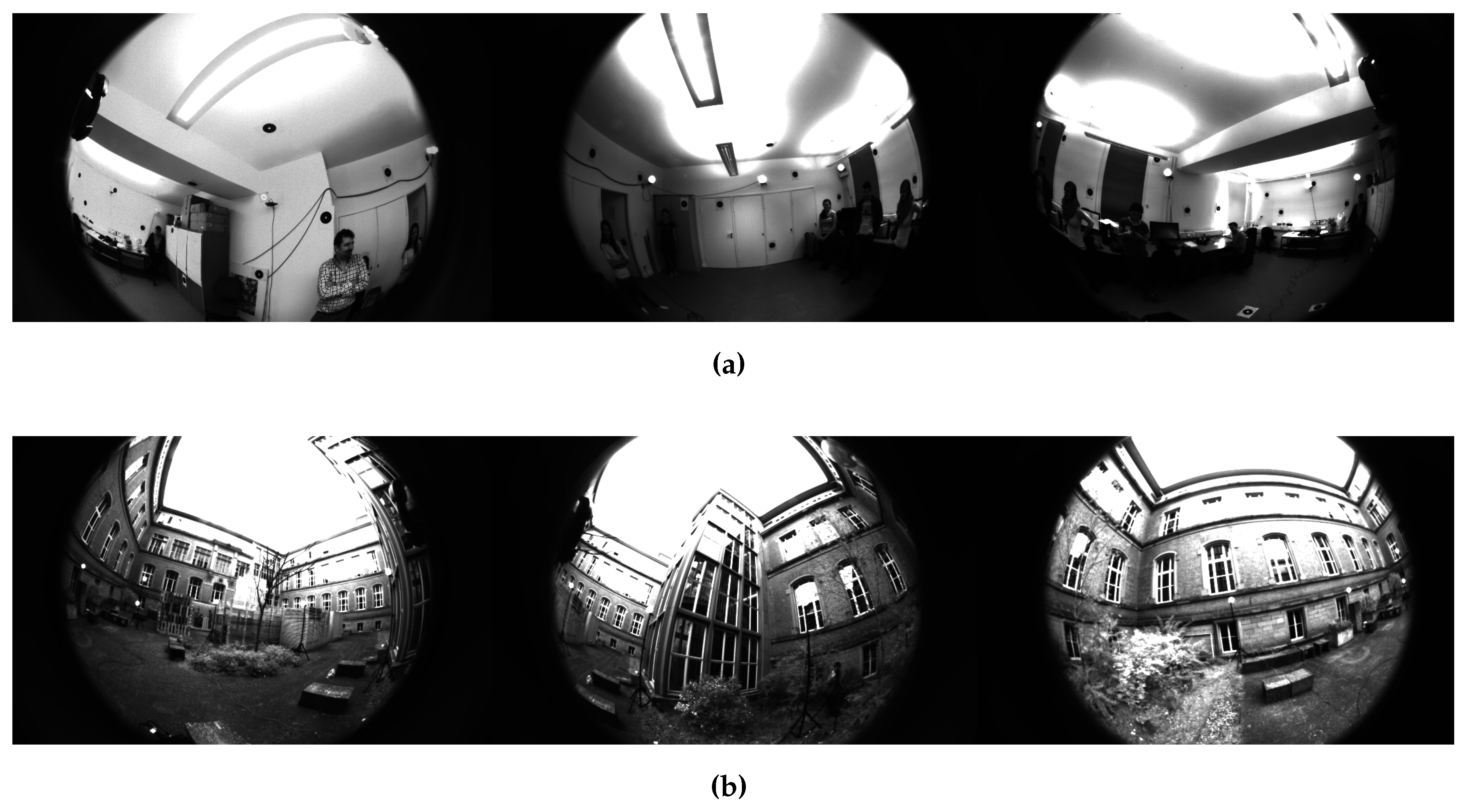
Figure 4.
Extrinsic laserscanner to fisheye camera calibration.

Figure 5.
Textured 3D model of the outdoor environment, reconstructed using AgiSoft Photoscan and about 500 high resolution images from a 36 Mpix DSLR camera. The images are also provided in the dataset.
Figure 5.
Textured 3D model of the outdoor environment, reconstructed using AgiSoft Photoscan and about 500 high resolution images from a 36 Mpix DSLR camera. The images are also provided in the dataset.


Table 1.
Overview of related datasets. GPS: Global Positioning System; INS: Inertial Navigation System; IMU: Inertial Measurement Unit.
| Dataset Name | Sensors | Indoor | Outdoor | Ground Truth Type |
|---|---|---|---|---|
| TUM RGB-D [1] | RGB-D | ✓ | Motion capture | |
| Monocular VO [3] | Fisheye, wide-angle cameras | ✓ | ✓ | Motion capture |
| KITTI [4] | Laserscanner, stereo cameras, GPS/INS | ✓ | GPS/INS | |
| EuRoC [5] | Stereo camera, IMU | ✓ | Motion capture/lasertracker | |
| Rawseeds [6] | Laserscanner, IMU, different cameras | ✓ | ✓ | Visual marker, GPS |
| Malaga [7] | Laserscanners, stereo cameras | ✓ | GPS | |
| New College [8] | Laserscanners, stereo & omnidirectional cameras | ✓ | None | |
| LaFiDa [this work] | Laserscanner, multi-fisheye cameras | ✓ | ✓ | Motion capture |
| Sensor | Specifications |
|---|---|
| Laserscanner | |
| Hokuyo UTM-30LX-EW | Field of view: 270° |
| Angular resolution: 0.25° | |
| Emitted laser pulses per scan line: 1080 | |
| Multi-echo-recordings up to 3 | |
| Wavelength: λ = 905 nm | |
| Maximum distance: 30 m | |
| Accuracy between 0.1 and 10 m: ±30 mm | |
| Weight: 210 g (without cable) | |
| Multi-fisheye camera system (MCS) | |
| VRmagic VRmC-12/BW OEM (USB-Platform) | Image size: 754 px × 480 px |
| Pixel size: 6 μm × 6 μm | |
| Maximum frame rate: 70 Hz | |
| Pixel clock: 13…27 MHz | |
| Lensagon BF2M12520 (Lenses) | Sensor: 1/3 in |
| Focal length: 1.25 mm | |
| Field of view: 185° | |
| Tracking system | |
| OptiTrack Prime 17 W | Image size: 1664 px × 1088 px |
| Pixel size: 5.5 μm × 5.5 μm | |
| Frame rate: 30–360 FPS (adjustable) | |
| Latency: 2.8 ms | |
| Shutter type: global | |
| Shutter speed: | |
| - Default: 500 μs (0.5 ms) | |
| - Minimum: 10 μs (0.01 ms) | |
| - Maximum: 2500 μs (2.5 ms) at 360 FPS |
Table 3.
Trajectory statistics: all are rounded and are supposed to give a rough impression of the trajectory characteristics. Depicted are the number of frames, the length in meters, the duration in seconds, and the average translation and rotation velocity. We omit some statistics for the trajectory Outdoor large loop, because most parts of the trajectory are outside the tracking volume of the motion capture system.
| Name | Number of Frames | Length (m) | Dur (s) | Avg m/s | Avg °/s | Number of Scan Lines | Point (106) |
|---|---|---|---|---|---|---|---|
| Indoor static | 1017 | 21 | 60 | 0.36 | 29 | 2333 | 2.52 |
| Indoor dynamic | 759 | 17 | 56 | 0.29 | 30 | 2609 | 2.82 |
| Outdoor rotation | 780 | 5 | 52 | 0.1 | 33 | 2176 | 2.35 |
| Outdoor static | 756 | 14 | 50 | 0.28 | 15 | 2609 | 2.30 |
| Outdoor static 2 | 1643 | 33 | 110 | 0.30 | 28 | 3755 | 3.84 |
| Outdoor large loop | 3177 | 00 | 225 | - | - | 7993 | 8.64 |
© 2017 by the authors; licensee MDPI, Basel, Switzerland. This article is an open access article distributed under the terms and conditions of the Creative Commons Attribution (CC-BY) license (http://creativecommons.org/licenses/by/4.0/).
Share and Cite
MDPI and ACS Style
Urban, S.; Jutzi, B. LaFiDa—A Laserscanner Multi-Fisheye Camera Dataset. J. Imaging 2017, 3, 5. https://doi.org/10.3390/jimaging3010005
AMA Style
Urban S, Jutzi B. LaFiDa—A Laserscanner Multi-Fisheye Camera Dataset. Journal of Imaging. 2017; 3(1):5. https://doi.org/10.3390/jimaging3010005
Chicago/Turabian StyleUrban, Steffen, and Boris Jutzi. 2017. "LaFiDa—A Laserscanner Multi-Fisheye Camera Dataset" Journal of Imaging 3, no. 1: 5. https://doi.org/10.3390/jimaging3010005
Note that from the first issue of 2016, this journal uses article numbers instead of page numbers. See further details here.