Next Article in Journal
3D Imaging with a Sonar Sensor and an Automated 3-Axes Frame for Selective Spraying in Controlled Conditions
Previous Article in Journal
Estimation Methods of the Point Spread Function Axial Position: A Comparative Computational Study
 
 
Erratum published on 23 June 2017, see J. Imaging 2017, 3(3), 23.
Article

Radial Distortion from Epipolar Constraint for Rectilinear Cameras

1
Department of Built Environment, Aalto University, P.O. Box 15800, 00076 Aalto, Finland
2
National Land Survey of Finland, Finnish Geospatial Research Institute FGI, PL 84, 00521 Helsinki, Finland
*
Author to whom correspondence should be addressed.
J. Imaging 2017, 3(1), 8; https://doi.org/10.3390/jimaging3010008
Submission received: 10 August 2016 / Revised: 11 January 2017 / Accepted: 13 January 2017 / Published: 24 January 2017

Abstract

:
Lens distortion causes difficulties for 3D reconstruction, when uncalibrated image sets with weak geometry are used. We show that the largest part of lens distortion, known as the radial distortion, can be estimated along with the center of distortion from the epipolar constraint separately and before bundle adjustment without any calibration rig. The estimate converges as more image pairs are added. Descriptor matched scale-invariant feature (SIFT) point pairs that contain false matches can readily be given to our algorithm, EPOS (EpiPOlar-based Solver), as input. The processing is automated to the point where EPOS solves the distortion whether its type is barrel or pincushion or reports if there is no need for correction.

Graphical Abstract

1. Introduction

The bottleneck in turning every consumer-grade digital camera into a 3D scanner is in how to automatically self-calibrate the lens distortion from arbitrary image pairs. In contrast to capturing objects by encircling them with a camera, which is a well-studied problem (see, e.g., [1]), problems arise when capturing large-scale (indoor) environments with minimum image overlap in order to reduce the effort of image acquisition. Such a method, if “black-boxed”, would enable multiple applications, for example, in real-estate management and brokering (see, e.g., [2]).
Lens distortion is a combination of lens properties and imperfections in the camera lens manufacturing process [3]. It is well known that lens distortion changes with the focal length, which in turn is altered by both zoom and focus settings. The first is significant, while the latter can be omitted beyond focused distances of around 15-times nominal focal length [4,5]. For zoom lenses, the form of distortion may change from barrel at the wide-end to pincushion at the tele-end. In other words, the sign of the radial distortion parameters may change with zoom. Computationally, this may be dealt with, e.g., by using two separate models [6].
The image processing in photogrammetry, traditionally, consists of two steps [7,8,9]. First, the lens distortion is solved in a camera calibration together with other interior orientation parameters that are the focal length and the principal point, or the center of distortion. A checkerboard [10], other calibration targets [11] or robust features [8] are used to ensure accuracy. Second, (sparse) 3D reconstruction of the wanted scene is made using bundle adjustment, usually from different images than what was used in the first step. The other way, which is popular in computer vision, is to streamline these two steps into one by embedding a non-linear lens distortion model directly into the 3D reconstruction bundle adjustment [12,13,14,15,16]. This way, same images can be used throughout the whole process, and some of the most important intrinsic camera parameters, such as the focal length, and the first two radial distortion coefficients can be recovered [14,17].
Despite the success of the one-step bundle adjustment, the inherent problem in the calculation of the reprojection error is that in addition to the lens distortion, also the external camera parameters and the parameters of the structure must be estimated. In other words, if one is first interested in only solving the lens distortion, the structure consisting of 3D points brings unwanted free parameters. This is especially problematic when attempting to reconstruct a large area with an uncalibrated camera, for example, in the built environment. Then, the camera network is loosely connected, i.e., it has weak geometry. Different unknown variables intertwine in bundle adjustment so that, for example, lens distortion deforms shapes in the object space [18]. Moreover, the effort of collecting data is unnecessarily increased by the requirement that all data must fulfill the redundancy requirement to solve lens distortion. Even if one prefers to perform a 3D reconstruction with minimal data, e.g., three images covering each point, it typically leads to having dozens or even hundreds of images. It would be beneficial if all of these available data could be used for the self-calibration of lens distortion. Therefore, it is evident that the lens distortion should be solved separately, before entering bundle adjustment.
The largest component of lens distortion is the radial component, in contrast to decentering and in-plane terms [19]. Radial lens distortion has an ordered correlation pattern, radial symmetry or r-symmetry, which can be detected, to some extent, with a blind approach for the purpose of removing this correlation [20], but in order to achieve further accuracy, more a priori knowledge is required. On the one hand, the epipolar constraint has been studied [21,22,23,24,25]. On the other hand, these studies typically rely on a single image pair, which as an approach contains the inherent need to control, not only noise, but also the scene properties in terms of appropriate feature detection, to avoid risks related to method instability. What has not been studied is utilizing multiple image pairs (that may also be from different scenes), which circumnavigates the problem by turning the question of stability, “whether an image pair is suitable for distortion detection”, into a question of convergence: “how many image pairs are needed to accurately detect the distortion”.
In this paper, we set out to exploit the r-symmetry in determining a global estimate for the radial distortion and, in order to do so, also construct a global constraint for the center of distortion that becomes more and more accurate as more image pairs are added. To our best knowledge, this has not been attempted before. We use uncalibrated images and present results for simulated data for multiple rectilinear lenses and zoom settings. In addition, real data containing false matches are used. The processing is automated to the point where our algorithm tells us whether the correction with the used model succeeds or if it is even needed.
The rest of this paper is organized as follows. In Section 2, the literature related to the lens distortion and the epipolar constraint is reviewed. In Section 3, as a continuation to this previous work, we show how epipolar constraints from different image pairs can be merged to estimate radial distortion. However, as this method depends on r-symmetry, it requires a good estimate for the center of distortion. Therefore, in Section 4, we introduce a new symmetry metric to obtain the estimate. Results are in Section 5, and the conclusion thereafter.

2. Related Work

Correcting the lens distortion before bundle adjustment (BA) reduces the amount of unknown parameters needed during it, thus increasing the robustness of the BA solution. Simultaneously, this paradigm allows an automated black-box-type use of the correction method; see the bottom arrow of Figure 1. For these reasons, it is meaningful to study what parts of distortion can be solved already with the singular image-pair correlation matrix, i.e., the fundamental matrix. The first attempt by Zhang [21] was to expand the epipolar constraint with a distortion function so that
u ˜ T F u ˜ = 0 ,
where u ˜ T = [ x ˜ , y ˜ , 1 ] and u ˜ T = [ x ˜ , y ˜ , 1 ] denote a pair of matching undistorted keypoints on two separate images, and F is the obtained fundamental matrix. The keypoints, in turn, are obtained from observations u T = [ x , y ] and u T = [ x , y ] by using a (radial) distortion correction
x ˜ = x D ( r ) y ˜ = y D ( r )
D ( r ) = 1 + k 1 r 2 ,
where r 2 = ( x x p ) 2 + ( y y p ) 2 . This first attempt was flawed in two ways. First, rigorously, the distortion center p = ( x p , y p ) is defined by the distortion model [26], meaning that for each lens distortion model, there exists a unique center of distortion specific for that model. However, in the work by Zhang [21], it was assumed to reside at the center of the image.
Second, the attempt by Zhang [21] and that of Fitzgibbon [22] relied on the so-called nine-point method for solving the fundamental matrix, which does not enforce the rank-two constraint. However, even in the studies by Kukelova and Pajdla [23] and Liu and Fang [24], where the rank-two constraint was enforced, the center of distortion was still assumed to be at the center of the image, i.e., the first flaw still persisted. We shall return to these issues in the next section.
Successful attempts to determine the location of the center of distortion have been made, although these are limited to specific conditions. Hartley and Kang [27] were able to construct a parameter-free distortion model with a center of distortion estimator by using a calibration rig, but their model, although theoretically sound, could not handle normal in situ noise without the rig. Brito et al. [25] used the curvature of epipolar lines to determine the location of the center of distortion, but this method’s success was limited to images with curvilinear lens-type distortion, i.e., very large distortion, due to problems in detecting differences in small curvatures. In addition, one-image pair methods typically experience vulnerabilities with respect to noise. According to Brito et al. [25] “with more than one pixel noise the given implementation produces very large errors”.
With multiple image pairs, however, these vulnerabilities related to noise, in addition to those related to false matches and inadequately distributed features, do not turn into a question of stability, but rather, into a question of convergence. All data, even from different scenes, can be used to converge the result. Therefore, the convergence of the radial distortion coefficient as a function of the number of inlier point pairs, or image pairs—since the amount of points per image is typically fixed by the natural properties of the scene— is of major importance.

3. Iterative Solution for Radial Distortion

To order to determine the lens distortion using multiple image pairs, we may extend Equation (1) as
min k 1 image pairs point pairs u ˜ T F u ˜ = ϵ ,
where vertical bars denote the L 1 norm. At the limit of no noise, ϵ 0 with an ideal distortion model. Despite its theoretical simplicity, Equation (4) typically contains difficult terms that follow from camera geometry, noise and false matches. We shall return to discuss these later.
Zhang’s idea of optimizing F and k 1 in consecutive loops, so that one variable is estimated and the other is kept fixed, and then vice versa until both converge separately, is bright, but not numerically stable for one pair of images [21]. However, we argue that this idea may well work for multiple image pairs, especially if the previous two flaws are overcome, i.e., the center of distortion is properly estimated (see Figure 2), and F’s rank-two constraint is enforced. Considering the first, we can then exploit r-symmetry properly. Considering the latter, the more data we have available, the more likely a larger area of the image plane is covered by the matching point pairs. Hence, k 1 cannot get in an artificial numerical coupling (caused by finite data) with a single F. Furthermore, as the amount of data grows, the statistical error in k 1 diminishes. This is, descriptively, something solid against which k 1 can converge.
Therefore, we make k 1 and all F k to converge in consecutive loops. In the following notation, we use image coordinates that are normalized with a = w / 4 to avoid F matrix ill-conditioning, where w is the image width in pixels. The symbol η is used to mark the counterpart of k 1 , to distinguish these two from each other. To obtain dimensionless quantities for comparison, we note that the distance from the center of distortion r = a r ^ , and η = η ^ / a 2 , where the ‘hat’ symbol stands for these dimensionless quantities.
Given a proposed center of distortion p p r and a radial distortion model
D ( r ) 1 + η r 2 ,
the distortion coefficient η is computed as follows.
The fundamental matrices F k and the respective inliers are computed from an initial set of point pairs u , u i using RANSAC and the proper rank-two constraint for F k (these initial observations are replaced on later iteration rounds with the corrected points u ˜ , u ˜ i , which is explained later). Image pairs are indexed with k, point pairs with i, and the inlier mask M indicates whether a point pair is an inlier or not, M k ( i ) = 1 or = 0 , respectively. To prevent systematic errors in F k computation, we require that at least 15 point pairs must be inliers, or otherwise, the corresponding image pair is omitted. This is similar to the amount presented in the work of Hartley and Kang [27], who theoretically determined that 80 points in a connected network of four images is needed to estimate (radial) distortion. In F k calculation, we employed the OpenCV implementation of RANSAC [28] with a tolerance distance of three pixels. Different confidence estimate values are tested in the Results Section with real data.
For each inlier point pair, we consider the point with the largest r, regardless on which of the two images it lies and, with a little abuse of notation, denote it by u. In other words, the distortion on the other image is yet neglected. For each u, extending its (radial) vector u from the proposed center of distortion p p r onto the epipolar line gives us the undistorted keypoint vector
u ˜ = u + e u cos α u ^ ,
where the angle α between u and the line perpendicular to the epipolar line is obtained as
cos α = u · ( e u ) u e u .
In Equation (6), u ^ = u u denotes a unit vector, and e is a vector from p p r to point e that is the closest point of u on the epipolar line; see Figure 3.
From Equation (5), we have
r ˜ = r ( 1 + η i r 2 ) η i = r ˜ r r 3 ,
where r ˜ | u ˜ | . Specifically, one trial value η i is obtained for each point pair i. The radial distortion coefficient is obtained by taking a logarithmic average
η = exp 1 N i N α i log η i ,
where N = α i , and the weights α i are either zero or one, so that only one third of the terms with the lowest absolute value η i are retained. Then, if the majority of all of the remaining η i were negative, η is also declared negative.
In selecting the terms within Equation (9), one third is a rough estimate based on the geometry that effectively circumnavigates the trouble caused by epipolar lines being close to parallel with radial lines (see Figure 3), which produces overly large values for η i . Moreover, this offers robustness with respect to noise and false matches present in in situ data, in contrast to the minimization criterion of Equation (4).
After solving η from Equation (9), the original uncorrected points are corrected with it, namely
u ˜ , u ˜ i = D ( η ) u , u i .
Here, the correction is applied to both (or all) images. However, due to the fact that the distortion on the other image was neglected before, the strength of the correction is prone to be underestimated. Because of this, when new fundamental matrices F k are obtained using corrected point pairs u ˜ , u ˜ i from Equation (10), the inlier mask M k computation may result in some of the inlier point pairs still being treated as outliers. Therefore, the process of solving new η and new F k needs to be repeated iteratively until convergence, which is reached when η is no longer underestimated. This, in turn, is seen from the fact that the amount of inliers in M k stops growing.
We summarize the convergence condition, i.e., when the iteration loop is exited. Original uncorrected points are corrected as in Equation (10) using the latest η of Equation (9) on each iteration round. New F k and their respective new inlier masks M k are computed based on these. Specifically, M k ( i ) = 1 or = 0 , if the point pair i is correlated, or is not correlated, via F k , respectively. Hence, as the value of η becomes less and less underestimated, the inlier set of corrected points grows on each iteration round d N , notation M d , as M 1 u ˜ , u ˜ i M 2 u ˜ , u ˜ i . . . u ˜ , u ˜ i , and when it stops growing, we have the convergence condition, namely
M d u ˜ , u ˜ i M d + 1 u ˜ , u ˜ i , d N .
See Figure 2b for an illustration of growing M d . The algorithm pipeline is outlined in Algorithm 1. Next, we introduce how to obtain a good estimate for p p r , which is required by Equation (6).
Algorithm 1 EPOS algorithm.
  • Extract initial point pairs from images
  • Find a proposition for the center of distortion (Section 4).
    (a)
      Determine inliers by calculating fundamental matrices.
    (b)
      Circle around the image, and use the inliers to find the bottom of the ‘symmetry valley’. See Figure 4.
    (c)
      Walk along the bottom of the valley.
    (d)
      Stop at the high gradient. Obtain p p r from here.
  • Given p p r , determine radial distortion (Section 3).
    (a)
      Compute fundamental matrices F k and inlier masks M k from u ˜ , u ˜ i , for all image pairs k.
    (b)
      Exit if the inlier amount in M k did not grow (not on the first round).
    (c)
      Obtain the distortion coefficient η from Equation (9).
    (d)
      Correct initial u , u i by plugging η in Equation (10) to obtain updated u ˜ , u ˜ i .
    (e)
      Go to 3 (a).
  • Locally search for better p p r using 3. Choose the best result according to the inlier percentage.

4. Finding the Center of Distortion

The radial distortion model of Equation (5) has an obvious one-dimensional symmetry, which we will use in introducing a new way to divide the two-dimensional problem of finding p = ( x p , y p ) in an easier form of two one-dimensional problems.

4.1. Symmetry Ratio Measure

To employ r-symmetry successfully in Section 3, the quality of a proposed center of distortion p p r should be measured solely in terms of whether it provides good r-symmetry. This is in contrast with the methods that rely on minimizing some Euclidean distance, BA for instance. We propose a weighted binary-form symmetry metric that is based on the notion on which side of its respective epipolar line a point lies. If a point is on the same side as the symmetry center, it carries a positive weight; otherwise, its weight is zero. Formally
Θ ( p p r ) = w , if r u 2 r e 2 0 , if r u 2 > r e 2 ,
where r u 2 = | u p p r | 2 is the squared distance from the proposed center of distortion p p r to the keypoint u, and r e 2 = | e p p r | 2 is the squared distance from p p r to the point e. See Figure 3. Point e resides on epipolar line u T F and is the closest point to u. The weight w ( 0 , 1 ] is the normalized dot product of r u and the vector from the keypoint u to the point e. Hence, point pairs with close to parallel vectors (“good geometry”) have a greater impact than pairs with close to orthogonal vectors (“bad geometry”).
Barrel distortion manifests in observations lying (ideally: only) on the far side of the epipolar line, farther away from the center than they should be. In an ideal case, the symmetry metric of Equation (12) is equivalent for all point pairs i, i.e., Θ i 0 , meaning barrel distortion, or Θ i = w i , meaning pincushion distortion.
In practice, however, exceptions occur due to noise and the properties of the used distortion model, for instance. To illustrate non-ideal symmetry, three feature points are shown in Figure 3, with Θ = 1 , 0 and ≈0.2, for u 1 , u 2 and u 3 , respectively. Thus, the symmetry measure for p p r , for a set of image pairs, can be written as
r s ( p p r ) = image pairs 1 W k i = 1 N k Θ i ,
where N k is the total amount of point pairs for the image pair k, and W k = 1 N k i = 1 N k w i is the respective total weight, including also pairs with r u 2 > r e 2 .
The best r-symmetry is found at the point p p r that minimizes (or maximizes) Equation (13), namely
arg min p p r r s ( p p r ) .
One key property of the r s measure of Equation (13) is that it can be computed quickly. It can be thought of as a symmetry ratio, as the value it can obtain is limited in the range [ 0 , 1 ] ; see Figure 4. For barrel distortion, for which η < 0 , a (blue) valley is formed around the spot where the best symmetry, i.e., the best p p r , resides. In contrast, a (red) ridge rises to mark non-optimal symmetry. For pincushion distortion, for which η > 0 , the ridge offers the best symmetry and valley the worst. The proposed center of distortion p p r is moved, as explained in Section 4.2, until the condition of Equation (14), i.e., the bottom of the valley (or the top of the ridge), is reached.

4.2. Symmetry Landscape

The center of distortion p = ( x p , y p ) is a two-variable unknown. The most important property of the symmetry measure of Equation (13) is that it allows us to separately solve these variables, when the problem is cast into polar coordinates. In particular, since both the ridge and the valley extend to infinity by the definition of Equation (12), their orientation can be detected from almost any perimeter drawn around the center of the image. The correct radial positioning along the bottom of the valley can then be considered. We thus proceed in two steps.
The orientation is solved first by looking for the bottom of the valley; see the green circular arrow shown in Figure 4. Specifically, a sufficiently large square of 0 . 25 side length that can be said to capture all centers of distortions is drawn around the image center, and the symmetry measure r s of Equation (13) is computed on discrete points { p m } that reside at the perimeter and are spaced 0 . 004 apart from each other (in w / 4 units). In other words, solving the whole 2D landscape is not necessary, since we can only compute the 1D perimeter. After obtaining each r s ( p m ) , we calculate a weighted orientation vector
v = m p m r s ,
and norm it v ^ = v v , in order to get the orientation of the valley v ^ . In practice, local averages for perimeter points are calculated using six nearest neighbors. The perimeter point with the lowest value is at the bottom of the symmetry valley and indicates its orientation.
Second, we solve the radius by walking along the bottom of the valley, starting from the perimeter, illustrated by the red arrow in Figure 4. Using the same discrete step size of 0 . 004 , r s is computed along a straight path to the origin. The gradient r s = d r s d r is computed using finite differences. The walk is halted at the point where the gradient diverts from its average by more than one standard deviation, r s ( r ) avg r s > σ . Hence, the radius is solved, and p p r is obtained from there.
Finally, there is no knowledge on whether the distortion that we are trying to solve should be of the type barrel or pincushion. Therefore, both the spot p p r and its mirror position on the other side of the image center must be evaluated. These two answers are then processed, and the one yielding more inliers is selected and ultimately tested against the convergence condition of Equation (11). Hence, only one model is required in contrast to using two models [6].

4.3. Local Search

For an initial p p r obtained from Section 4.2, a local search algorithm was used to pinpoint the best location for the center of distortion. Trial steps with a discrete step size of 0 . 002 were made in four directions, two perpendicular and two parallel to the radius. If the amount of inliers obtained through the solution of Section 3 remained the same, the step size was increased by 10%. The walk was terminated when no further improvement in terms of inliers was found. Experimentally, we found that the local search improved the result in terms of η, although the local walks were short.

4.4. Implementation of the Proposed Method: EPOS

Our program EPOS (EpiPOlar-based Solver) is built so that it can automatically know whether it has actually managed to correct the lens distortion or whether it has failed to do so. This is done by simply comparing the amount of point pair inliers obtained with and without correction, using Algorithm 1. Distortion correction is considered successful if the amount of inliers has increased. In practice, we have two non-zero values of η, one for the minimum and one for the maximum of the symmetry measure (see Equation (14) and Figure 4), and the comparison is done also between these two; and against the no correction case.
The robustness of the implementation is built on a three-fold foundation. First, the computation of the fundamental matrix F enforces the rank-two constraint. Second, the symmetry metric to estimate the center of distortion is based on a majority voting that, in contrast to Euclidean-based measures, does not contain overly large, nor “diverging” terms arising from noise and false matches. Third, the radial distortion coefficient is evaluated from the most conservative third of point pairs, which circumnavigates the troublesome geometry when the epipolar lines are parallel to the radial lines.
Descriptor matched SIFT [29] features, such as those that are used for bundler input [30], can also be given to EPOS as input. False matches are handled in fundamental matrix computation as described in Section 3. Currently, the method’s convergence may be stopped if the F computation fails so that totally wrong F’s are present in the input. This is, however, a known problem for which solutions exist and beyond the scope of this paper. Considering the future work, one promising approach to decrease computation time and to further increase the method’s robustness with respect to F computation stability is to use graph-based point tracking [31] that minimizes the amount of initial data by reducing false matches from it.

4.5. Extension to Non-Rectilinear Lenses

Brown’s [3] thin lens approximation, derived as a Taylor approximation from the analytical ray tracing formula, holds only for weak distortion, cf. Equation (5). Some digital cameras, however, employ a fish-eye lens instead of a rectilinear (thin) lens. The fish-eye lens, alongside having a different distortion model than its rectilinear counterpart, differs also by not having a uniquely-defined center of projection, which may break down the whole pin-hole camera model if this effect is significant ([32], p. 242). If not, the fish-eye lens data may be corrected with EPOS if the mapping used by the lens model, stereographic for example, is known, and the images are first transformed into the rectilinear presentation. However, experiments with fish-eye lenses are beyond the scope of this work.

5. Results and Discussion

Methods relying on just one image pair are vulnerable to bad geometry and noise as already discussed in Section 2. With multiple image pairs, we speak of convergence and use a checkerboard to obtain simulated data for a thorough testing of the properties of EPOS. Choosing simulated data this way allows us to explore the relevant range for the distortion parameter that is used for off-the-shelf digital cameras that have rectilinear lenses.

5.1. Simulated Data

The convergence of η as a function of the number of inlier point pairs (the amount of points per image is fixed here to 49 due to the checkerboard) is shown in Figure 5, with a numerical summary in Table 1. For each image set size, ten results are computed to study the statistical behavior of the algorithm. These are obtained by drawing random subsets of image pairs from the checkerboard set. In Figure 5, the thick line follows the best inlier percentage and is drawn to guide the eye. Expectedly, yet remarkably, adding more data yields a better result as η converges to the reference result for different lenses. The impact of unstable interior orientation is well visualized, as the inexpensive zoomable 18–105-mm lens attached to the Panasonic DMC yields the slowest convergence. The same keypoint observations are used for testing EPOS and for obtaining reference results. Each image block is treated separately with respect to the lens model and zoom setting. Results for the center of distortion, shown in Figure 6, are discussed briefly. A sample checkerboard image is shown in Figure 7. Reference results were computed with the Caltech Camera Calibration Toolbox [10]. Reference values for k 1 are in pixels per focal length units, while EPOS η values are in the chosen pixel per w / 4 units. For result comparison, η results are transformed into k 1 units in Figure 5 and Table 1 by using a multiplication factor γ ² = ( f / a ) 2 , where f is the focal length from reference bundle adjustment, and a = w / 4 is the chosen unit scale in EPOS.
In order to verify how well EPOS handles the change of sign in η, we computed results for four different zoom values 24 mm, 28 mm, 35 mm and 50 mm, using a camera with stable interior orientation, Nikon D700 with a 24–70 mm objective; see Figure 5b. Convergence is achieved quickly, mostly because of the quality of the objective. At the limit of very small distortions and with a limited set of point pairs, there is a possibility that the set of point pairs is determined to all be inliers by RANSAC before EPOS enters the iterative solution loop. Then, EPOS decides that no improvement is required. Otherwise, the result converges at the limit, where the amount of point pairs is large.
In Figure 6a, the results for the center of distortion are shown for various image block sizes. The size of the point represents the amount of data used to calculate that point. All samples are weighted with inlier percentages, and these weighted averages are shown in Figure 6b. Again, the amount of inliers for each result is determined by the convergence condition of Equation (11). The fact that the recovered center of distortion is different from the reference result is noteworthy and follows from that these center of distortions actually have different definitions (remember the work of [26]). Rigorously put in other words, the proposed r-symmetry center is to be used only for lens distortion correction and not for any 3D measurements done afterwards, for which the principal point is the correct choice.
After obtaining η, the importance of the center of distortion diminishes. In order to see this, we undistorted the checkerboard images with one fixed value of η, but employed three different center of distortion values, which were the image center, the reference result and the result obtained from EPOS. Then, for each of these three undistorted image sets, we checked with the Caltech Calibration Toolbox that they all contained an essentially equivalent (and small) image distortion. Hence, even if the center of distortion plays a crucial role in solving the radial distortion parameter, as discussed in Section 4, its significance at the image correction phase is negligible, at least for the used distortion model.
The symmetry ratio plot in Figure 4 sheds light on the different centers of distortions shown in Figure 6b. The result from EPOS resides on the bottom of the deepest valley. The reference center of distortion resides at the bottom of another valley. In other words, multiple valleys and ridges may be present. This non-convex nature of the landscape highlights the importance of the ‘light-weight’ method of Section 4.2 to find the center of distortion efficiently. The data for Figure 4 were obtained from a set of 10 images, yielding 45 image pairs with a total of 2200 point pairs. For a smaller set of point pairs, the symmetry ratio surface becomes noisy, which also affects the convergence rate of η shown in Figure 5.

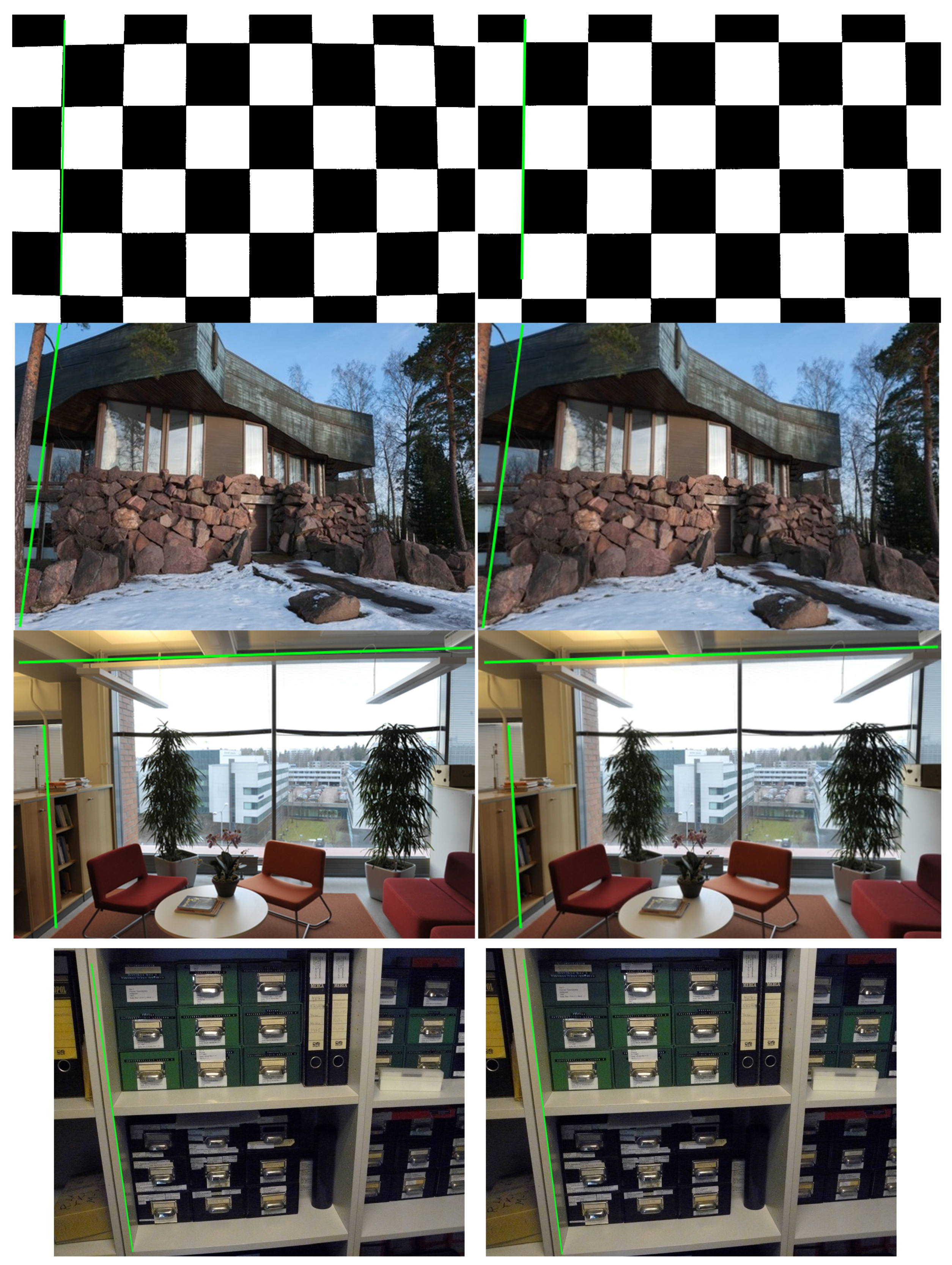
5.2. Real Data from In Situ Images

In order to validate EPOS beyond the simulated data that do not contain false matches, we captured images from built environment (or man-made environment). The Aalto University building named Dipoli and a set of sofas with challenging lighting and low-texture surfaces were shot with a hand-held D700 24 mm, resulting in sets of 10 and nine images, respectively, which were then resized to 532 × 354 pixels. In other words, we chose the lens with the smallest radial distortion and, in addition, notably reduce the image size to further challenge the proposed method. As the images were small, the F computation tolerance distance was reduced from three to two pixels. Using descriptor-matched SIFT feature coordinates, point pair data were given to EPOS as input. False matches and bad camera network geometry are both present. Results are summarized in Table 2 and the corresponding corrections of the images samples shown in Figure 7.
We study the impact of the confidence level parameter in fundamental matrix calculation. Obviously, a high confidence level requirement reduces the risk that the epipoles are displaced, but we also test the numerical precision of the method with respect to this parameter. For the Dipoli set, we obtain η = 0 . 0052 with the confidence value of 0 . 99 . With a lower confidence value of 0 . 95 , EPOS occasionally fails to present a result due to problems in F-matrix calculation. With a confidence value of 0 . 9 , most calculations fail producing a result of η = 0 , except for sets of six and around 14 image pairs that yield η = 0 . 0052 ± 5 % . For the sofa set, SIFT matching yields a total of 1568 initial point pairs, from which EPOS finds about 1250 inliers without radial distortion correction. With correction, EPOS finds about 1270 inliers, leaving 19 % of the point pairs as outliers. The difference in inlier amount is quite small between these two, so we tested the numerical stability of the result by using different confidence values in the fundamental matrix calculation. For confidence values of 0 . 90 , 0 . 95 and 0 . 99 , we obtain 0 . 0087 , 0 . 0067 and 0 . 0071 . Relative error for η is estimated here to reside within 15 % . We emphasize that these are very challenging sets of data.
With in situ images, typically a minimum of four image pairs is required to obtain the first decent result for η. In order to see if EPOS can truly handle image pairs from different scenes, we create a combined set from the previous Dipoli and sofa sets, taking the first three images from each. After F matrix calculation, this yields five image pairs. We obtain η = 0 . 0071 , which is remarkably close to the ground truth 0 . 0068 . The confidence values of 0 . 95 and 0 . 99 yielded this same result. The difference in results with this and the pure Dipoli set may be explained by the fact that features in Dipoli images are mainly on the center of the image, whereas the accurate recovery of the radial distortion requires also features near the image boundaries (as in the sofa set).
Images taken with the lens having the largest distortion, Panasonic DMC FZ8 6 mm, were reduced to 768 × 576 resolution, and the obtained SIFT matches were given to EPOS. With only five bookshelf images (equaling 10 image pairs), we obtain η = 0 . 0050 for both 0 . 95 and 0 . 99 confidence values; see Figure 7. The result stays within ± 4 % even if the amount of point pairs is increased from that of four image pairs ( 670 , 590 , 1690 ) to that of 10 image pairs ( 1858 , 1697 , 4939 ) , indicating pairs after correction, before correction and after SIFT match. Note that 62 % of the point pairs are outliers. Even for a 0 . 90 confidence value, a value of η = 0 . 0051 is ultimately obtained. The value of η obtained from these in situ images is quite close to the reference result η = 0 . 0072 (shown in different units k 1 = 0 . 1320 in Figure 5), and it leads to a rather good visual undistortion result; see the green lines in Figure 7.
In Table 2, our results are compared against a state-of-the-art BA-based open method, VisualSFM (VSFM) [33], which paradigmatically relates to the middle horizontal arrow in Figure 1. Similar to EPOS, VSFM employs only one radial distortion coefficient to estimate lens distortion. The methods perform equally well for the Dipoli set, where a good image network may be formed. On the bookshelf set, the VSFM estimate for η misses with a decade, while the accuracy of EPOS remains the same. Ultimately, the sofa set and the combined set have such a bad image geometry that VSFM fails to construct a image network and simultaneously to compute a good estimate for the focal length, which leads to radial distortion being unable to be reliably estimated. This can be seen from Table 2, where the ‘VSFM #’ image network size for these sets is be much smaller than the original size of the dataset, ‘# images’. On the other hand, EPOS performs well. Note that EPOS does not need to compute the focal length f, in contrast to BA-based methods, such as the VSFM or the Caltech Toolbox used to compute the reference results. Another difference is that EPOS does not require an image network of good geometry, but can operate on image pairs only. Finally, note that the reference values for f and η in Table 2 are the same as for Figure 5.
We conclude that EPOS is robust to noise, but also to false matches. However, if false matches are so abundant that the fundamental matrix calculation results in a wrong F with significantly displaced epipoles, this (obviously) prevents the algorithm convergence by making the majority voting for the center of distortion location fail. Beyond the measures taken here, this risk may further be reduced by preparing the initial data with, e.g., graph-based point tracking [31].

5.3. Computational Efficiency

Considering the absolute consumed CPU time, a run with 500 point pairs is processed in about 80 s of CPU time on a single 3 . 0 -GHz core. Considering Figure 5, this corresponds to about 10–12 images. Good results can be obtained with simulated, but also with real datasets of this or a smaller size; see Figure 5 and Table 2, respectively. With real data, Table 2, current unoptimized processing times for the single CPU, full dataset, single runs were 10 min for Dipoli, 4 . 4 min for sofa, 68 s for combined and 10 min for bookshelf (with fewer, but larger images than Dipoli). Considering the scaling properties of the proposed method beyond this, a practical level of convergence is reached already at the image set sizes of 20; see Figure 5. Improving the computational efficiency by parallel processing and code optimization towards real-time performance will be done as a part of the future work.

6. Conclusions

We have presented a solution for correcting lens distortion from uncalibrated images using the epipolar constraint without any calibration rig. The solution employs r-symmetry to build a global constraint that works even for image networks with bad geometry. As a consequence, the same images may be first used to calibrate the camera for lens distortion in a separate pre-processing step, and then used for 3D reconstruction purposes. Our EpiPOlar-based Solver, or EPOS, is fully automated and benefits from multiple image pairs. EPOS delivers a negative (positive) radial distortion parameter for barrel (pincushion) distortion or it decides that no correction is needed. When the amount of data is increased, EPOS yields a converging result for the distortion model, which currently consists of the one radial distortion parameter and the center of distortion. Feature-matched SIFT points containing false matches can be used as input data. With sufficient data, the rate of convergence is dictated by the stability of the camera’s interior orientation, i.e., the physical properties of the camera. Future work includes the optimization of the EPOS code, extending it for fish-eye lenses, and the introduction of more complex, multi-parameter correction models. We plan to publish the method in an open repository (https://github.com/vlehtola/rsymmetryEPOS).

Acknowledgments

The authors wish to thank the Academy of Finland for funding this research, Grant Nos. 257755, 272195, and 293389.

Author Contributions

V.L. developed and implemented the proposed algorithm, and wrote the first draft of the article. M.K. designed the setup for the simulated data, and produced the reference results. P.R. contributed soundly to the theoretical part, which was put together with V.L. All authors revised the final version of the article.

Conflicts of Interest

The authors declare no conflict of interest.

References

  1. Nicolae, C.; Nocerino, E.; Menna, F.; Remondino, F. Photogrammetry applied to Problematic artefacts. Int. Arch. Photogramm. Remote Sens. Spat. Inf. Sci. 2014, 40, 451–456. [Google Scholar] [CrossRef]
  2. Lehtola, V.V.; Kurkela, M.; Hyyppä, H. Automated image-based reconstruction of building interiors—A case study. Photogramm. J. Finl. 2014, 1, 1–13. [Google Scholar] [CrossRef]
  3. Brown, D.C. Close-range camera calibration. Photogramm. Eng. 1971, 37, 855–866. [Google Scholar]
  4. Fryer, J.G.; Brown, D.C. Lens distortion for close-range photogrammetry. Photogramm. Eng. Remote Sens. 1986, 52, 51–58. [Google Scholar]
  5. Fraser, C.; Shortis, M. Variation of distortion within the photographic field. Photogramm. Eng. Remote Sens. 1992, 58, 851–855. [Google Scholar]
  6. Kim, D.; Shin, H.; Oh, J.; Sohn, K. Automatic radial distortion correction in zoom lens video camera. J. Electron. Imaging 2010, 19, 043010. [Google Scholar] [CrossRef]
  7. Fraser, C.; Al-Ajlouni, S. Zoom-dependent camera calibration in digital close-range photogrammetry. Photogramm. Eng. Remote Sens. 2006, 72, 1017–1026. [Google Scholar] [CrossRef]
  8. Remondino, F.; Fraser, C. Digital camera calibration methods: considerations and comparisons. Int. Arch. Photogramm. Remote Sens. Spat. Inf. Sci. 2006, 36, 266–272. [Google Scholar]
  9. Strecha, C.; Hansen, W.V.; Gool, L.V.; Fua, P.; Thoennessen, U. On Benchmarking Camera Calibration and Multi-View Stereo for High Resolution Imagery. In Proceedings of the IEEE Conference on Computer Vision and Pattern Recognition, CVPR 2008, Anchorage, AK, USA, 23–28 June 2008; pp. 1–8.
  10. Bouguet, J.Y. Camera Calibration Toolbox for Matlab. Available online: http://www.vision.caltech.edu/bouguetj/calib_doc/ (accessed on 1 July 2016).
  11. Photometrix. Australis—Camera Calibration Software. Available online: http://www.photometrix.com.au/australis/ (accessed on 1 July 2016).
  12. Jeong, Y.; Nister, D.; Steedly, D.; Szeliski, R.; Kweon, I. Pushing the Envelope of Modern Methods for Bundle Adjustment. IEEE Trans. Pattern Anal. Mach. Intell. 2012, 34, 1605–1617. [Google Scholar] [CrossRef] [PubMed]
  13. Wu, C.; Agarwal, S.; Curless, B.; Seitz, S.M. Multicore Bundle Adjustment. In Proceedings of the 2011 IEEE Conference on Computer Vision and Pattern Recognition (CVPR), Colorado Springs, CO, USA, 20–25 June 2011; pp. 3057–3064.
  14. Lourakis, M.I.A.; Argyros, A.A. SBA: A software package for generic sparse bundle adjustment. ACM Trans. Math. Softw. 2009, 36, 1–30. [Google Scholar] [CrossRef]
  15. Furukawa, Y.; Ponce, J. Accurate Camera Calibration from Multi-View Stereo and Bundle Adjustment. In Proceedings of the IEEE Conference on Computer Vision and Pattern Recognition, CVPR 2008, Anchorage, AK, USA, 23–28 June 2008; pp. 1–8.
  16. Snavely, N.; Seitz, S.; Szeliski, R. Photo Tourism: Exploring Photo Collections in 3D. ACM Trans. Graph. (TOG) 2006, 25, 835–846. [Google Scholar] [CrossRef]
  17. Zhang, Z. A flexible new technique for camera calibration. IEEE Trans. Pattern Anal. Mach. Intell. 2000, 22, 1330–1334. [Google Scholar] [CrossRef]
  18. Wu, C. Critical Configurations for Radial Distortion Self-Calibration. In Proceedings of the 2014 IEEE Conference on Computer Vision and Pattern Recognition (CVPR), Columbus, OH, USA, 23–28 June 2014.
  19. Fraser, C.S. Automatic camera calibration in close range photogrammetry. Photogramm. Eng. Remote Sens. 2013, 79, 381–388. [Google Scholar] [CrossRef]
  20. Farid, H.; Popescu, A.C. Blind removal of lens distortion. J. Opt. Soc. Am. A 2001, 18, 2072–2078. [Google Scholar] [CrossRef]
  21. Zhang, Z. On the Epipolar Geometry between Two Images with Lens Distortion. In Proceedings of the 13th International Conference on Pattern Recognition, Vienna, Austria, 25–29 August 1996; Volume 1, pp. 407–411.
  22. Fitzgibbon, A.W. Simultaneous Linear Estimation of Multiple View Geometry and Lens Distortion. In Proceedings of the 2001 IEEE Computer Society Conference on Computer Vision and Pattern Recognition, CVPR 2001, Kauai, HI, USA, 8–14 December 2001; Volume 1, pp. 125–132.
  23. Kukelova, Z.; Pajdla, T. A Minimal Solution to Radial Distortion Autocalibration. IEEE Trans. Pattern Anal. Mach. Intell. 2011, 33, 2410–2422. [Google Scholar] [CrossRef] [PubMed]
  24. Liu, X.; Fang, S. Correcting large lens radial distortion using epipolar constraint. Appl. Opt. 2014, 53, 7355–7361. [Google Scholar] [CrossRef] [PubMed]
  25. Brito, J.H.; Angst, R.; Koser, K.; Pollefeys, M. Radial Distortion Self-Calibration. In Proceedings of the 2013 IEEE Conference on Computer Vision and Pattern Recognition (CVPR), Portland, OR, USA, 23–28 June 2013; pp. 1368–1375.
  26. Willson, R.G.; Shafer, S.A. What is the center of the image? J. Opt. Soc. Am. A 1994, 11, 2946–2955. [Google Scholar] [CrossRef]
  27. Hartley, R.; Kang, S.B. Parameter-free radial distortion correction with center of distortion estimation. IEEE Trans. Pattern Anal. Mach. Intell. 2007, 29, 1309–1321. [Google Scholar] [CrossRef] [PubMed]
  28. Fischler, M.A.; Bolles, R.C. Random sample consensus: A paradigm for model fitting with applications to image analysis and automated cartography. Commun. ACM 1981, 24, 381–395. [Google Scholar] [CrossRef]
  29. Lowe, D. Distinctive Image Features from Scale-Invariant Keypoints. Int. J. Comput. Vis. 2004, 60, 91–110. [Google Scholar] [CrossRef]
  30. Snavely, N. Bundler: Structure from Motion (SFM) for Unordered Image Collections. Available online: http://www.cs.cornell.edu/ snavely/bundler/ (accessed on 11 October 2014).
  31. Olsson, C.; Enqvist, O. Stable Structure from Motion for Unordered Image Collections; Springer: Berlin/Heidelberg, Germany, 2011; Volume 6688, pp. 524–535. [Google Scholar]
  32. McGlone, C.; Mikhail, E.; Bethel, J. Manual of Photogrammetry, 5th ed.; American Society of Photogrammetry: Bethesda, MD, USA, 2005. [Google Scholar]
  33. Wu, C. VisualSFM: A Visual Structure from Motion System. Available online: http://ccwu.me/vsfm/doc.html (accessed 1 July 2016).
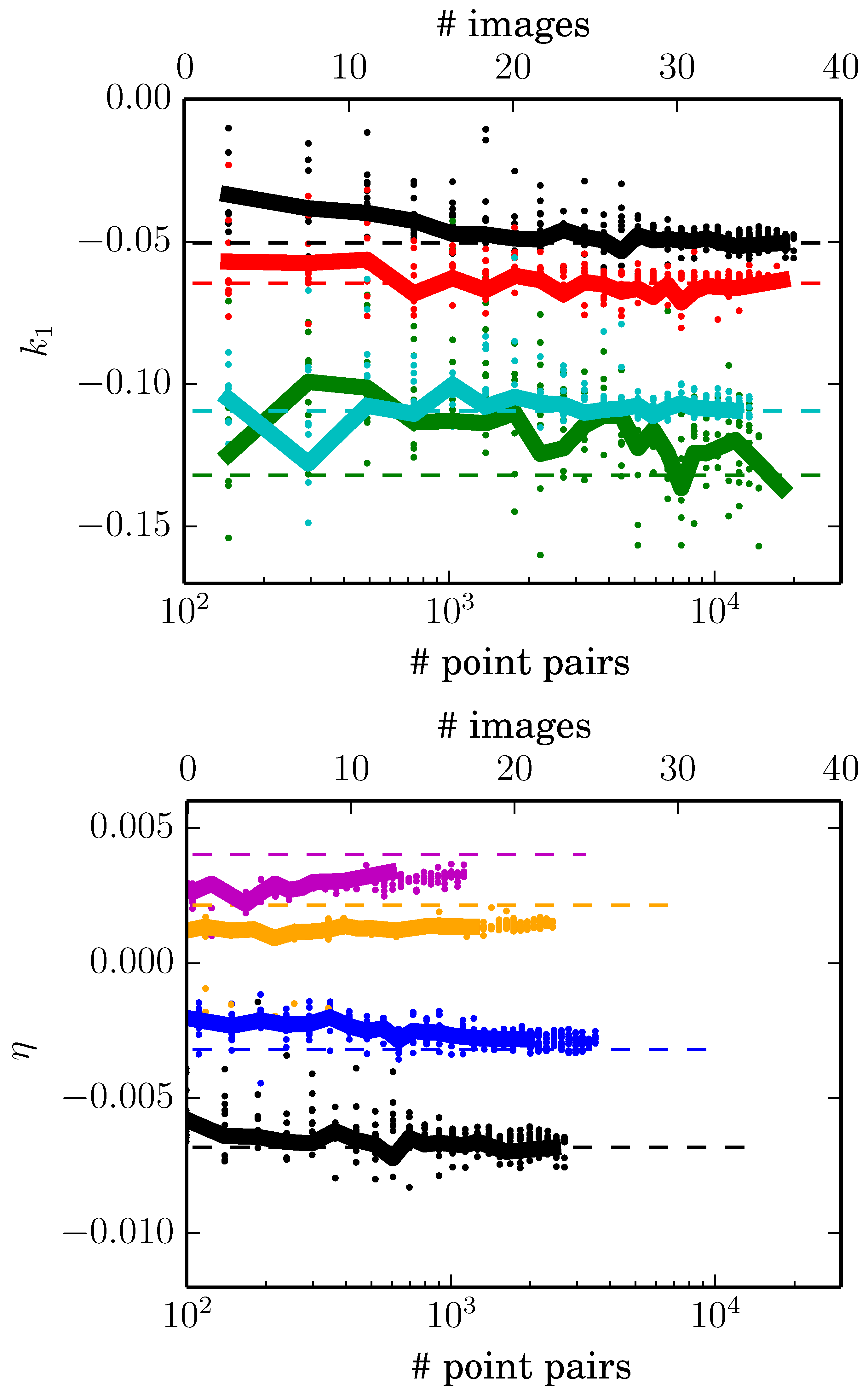
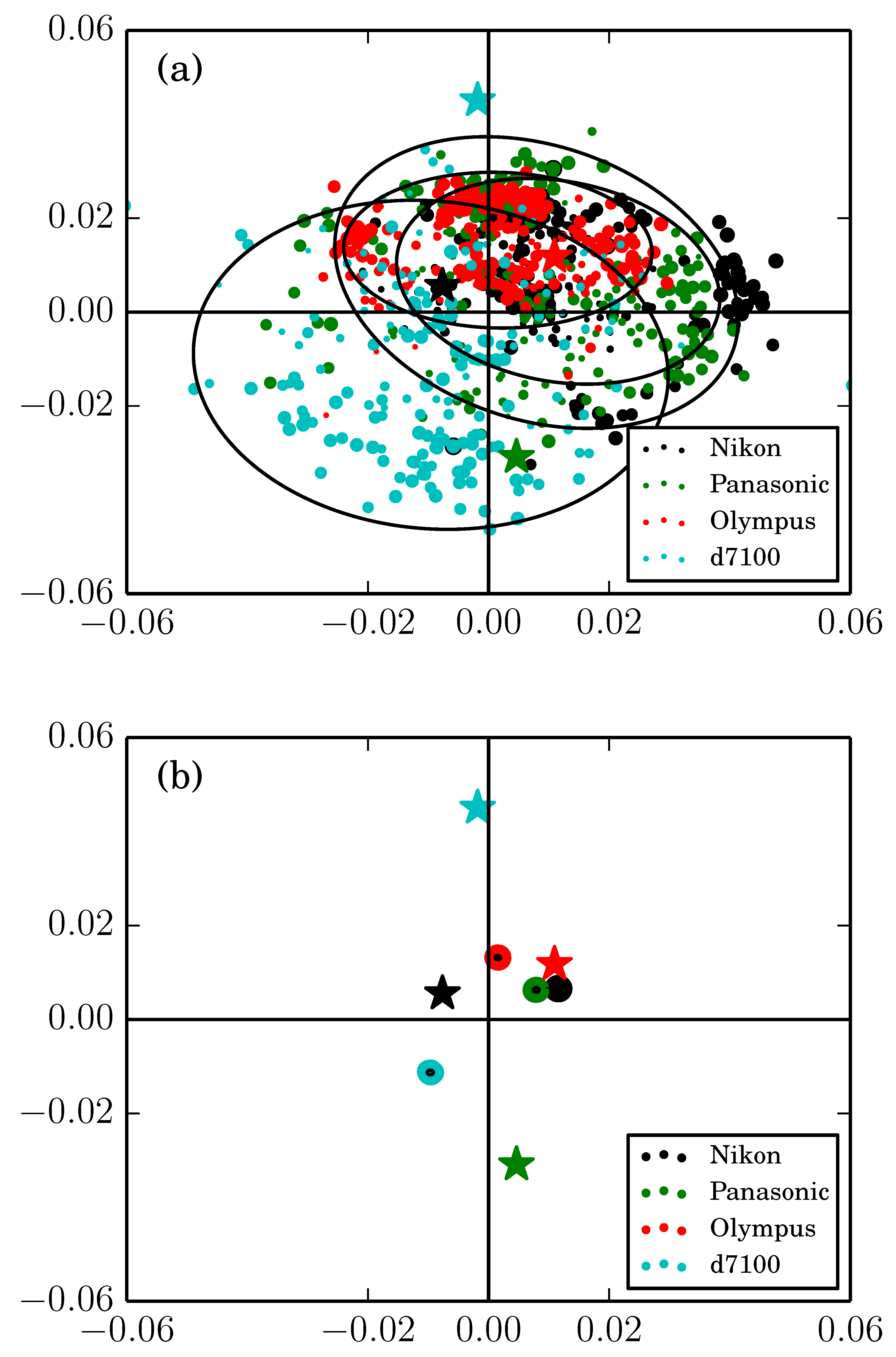
Figure 1. The proposed method, and its implementation EPOS, introduce a new automated ‘black-box’ paradigm in solving lens distortion for image sets with weak geometry, compared to the existing alternatives of either using a pre-calibrated camera (top arrow) or employing a non-linear distortion correction term inside bundle adjustment (middle arrow).
Jimaging 03 00008 g001
Figure 2. Illustrations of radial symmetry; see Equation (5). (a) Barrel distortion, η < 0 ; (b) pincushion distortion with a (magenta) center of distortion different from the (black) center of the image. Symmetry is employed while solving the fundamental matrices F k and the radial correction parameter of Equation (9) consecutively. Here, each iteration increases the amount of inliers, M 1 < M 2 < M 3 < . . . , until the convergence of Equation (11) is reached, and η > 0 is obtained.
Jimaging 03 00008 g002
Figure 3. Properties for observations u i and their respective epipolar lines (black solid lines). The radial correction function works best when the radial vector is perpendicular to its respective epipolar line, such as u 1 , pointing from p to u 1 , because the geometry is then optimal. Then, the intersection of the radial vector and the epipolar line is, at the same time, the closest point on the line, u ˜ 1 = e 1 . In contrast, the radial vector of point u 3 is almost parallel to its respective epipolar line. Here, the function is bound to overestimate the correction, even if the closest point on the line e 3 is close to u 3 . The most typical case u 2 is in between the previous two. The center of distortion p differs from the center of the image c = ( w / 2 , h / 2 ) .
Jimaging 03 00008 g003
Figure 4. Energy surface depicting the symmetry ratio r s = r s ( p p r ) , where the x- and y-axes span the location of p p r . A low/blue (high/red) ratio indicates a favorable (unfavorable) position for p p r in terms of barrel distortion symmetry. The surface is non-convex. The best trial for the center of distortion p p r is found at the bottom of the valley. The EPOS result is shown with a big (green) dot in the deepest valley. The (black) dot on the ridge represents its mirror location. The reference result from bundle adjustment (BA) is shown with a big star in an upper valley. Green and red dotted lines represent how the scouting of the symmetry landscape is done; see Section 4.2.
Jimaging 03 00008 g004
Figure 5. Convergence of the value of η as a function of the number of inlier point pairs (and number of images). Note that as the checkerboard images form a connected network, a set of five or 20 images equals about 490 or 9310 point pairs, respectively. In other words, the amount of point pairs grows exponentially with respect to the amount of images. The dashed lines represent reference results onto which the results from EPOS (solid lines) converge. The previous, in top to bottom order, are (a) Nikon D700 24 mm, Olympus 14 mm, Nikon D7100 18 mm, Panasonic DMC 6 mm; (b) results for four different zoom settings, 24 mm, 28 mm, 35 mm and 50 mm, for Nikon D700 (bottom to top order). Note the different units for η and k 1 ; see the text for details.
Jimaging 03 00008 g005
Figure 6. (a) Center of distortion results from EPOS are shown as dots, while reference results are marked as stars. Ellipses describe sample variances; (b) The same data displayed through weighted sample averages with reference results. See the text for details.
Jimaging 03 00008 g006
Figure 7. Results from EPOS. Distorted (left) and undistorted (right) images for D700 24 mm. The checkerboard image (top) is corrected using the converged value of η obtained from checkerboard data; see Figure 5. The image colors were simplified to black and white for visual reasons. Sample images of a building called Dipoli (second from top) and a sofa set (third from top) are corrected with values obtained from the respective sets. Bookshelf images taken with the Panasonic 6 mm lens are also corrected with the value obtained in situ. Dipoli set contains 11 photos, the sofa set 9 photos and the bookshelf set 5 photos. Real-world cases contain false matches and were chosen to be quite difficult.
Jimaging 03 00008 g007
Table 1. Summary of the results shown in Figure 5. Averages k 1 and η are taken over the data for which # images ≥20, except for 50 mm over the data, for which # images ≥10.
Data Set Figure 5a k 1 Std dev (EPOS)Reference k 1
Nikon D700 24 mm−0.048680.00273−0.05038
Olympus 14 mm−0.063190.00271−0.06460
Nikon D7100 18 mm−0.107480.00257−0.10949
Panasonic DMC 6 mm−0.121070.01227−0.13201
Dataset Figure 5b η Std dev (EPOS)Reference η
24 mm−0.006590.00037−0.00681
28 mm−0.002820.00025−0.00319
35 mm0.001390.000150.00213
50 mm0.003080.000220.00402
Table 2. EPOS results with real data using a confidence value of 0 . 99 are compared against the state-of-the-art VisualSFM (VSFM) software.
Data Set# ImagesVSFM #VSFM fReference fRef. ηEPOS ηVSFM η
Dipoli1010372.2361.5 0 . 0068 0 . 0052 ± 5 % ( ) 0 . 0048
Sofa92354.6361.5 0 . 0068 0 . 0071 ± 15 % N/A
Combined 3 + 3 3602.0361.5 0 . 0068 0 . 0071 ± 10 % N/A
Bookshelf55803.6821.7 0 . 0072 0 . 0050 ± 4 % ( ) 0 . 00039

