Investigating the Influence of Box-Constraints on the Solution of a Total Variation Model via an Efficient Primal-Dual Method

Department of Mathematics, University of Stuttgart, Pfaffenwaldring 57, 70569 Stuttgart, Germany
J. Imaging 2018, 4(1), 12; https://doi.org/10.3390/jimaging4010012
Submission received: 2 October 2017
/
Revised: 2 January 2018
/
Accepted: 3 January 2018
/
Published: 6 January 2018
Abstract
:In this paper, we investigate the usefulness of adding a box-constraint to the minimization of functionals consisting of a data-fidelity term and a total variation regularization term. In particular, we show that in certain applications an additional box-constraint does not effect the solution at all, i.e., the solution is the same whether a box-constraint is used or not. On the contrary, i.e., for applications where a box-constraint may have influence on the solution, we investigate how much it effects the quality of the restoration, especially when the regularization parameter, which weights the importance of the data term and the regularizer, is chosen suitable. In particular, for such applications, we consider the case of a squared data-fidelity term. For computing a minimizer of the respective box-constrained optimization problems a primal-dual semi-smooth Newton method is presented, which guarantees superlinear convergence.
1. Introduction
An observed image g, which contains additive Gaussian noise with zero mean and standard deviation , may be modeled as
where is the original image, K is a linear bounded operator and n represents the noise. With the aim of preserving edges in images in [1] total variation regularization in image restoration was proposed. Based on this approach and assuming that and , a good approximation of is usually obtained by solving
where is a simply connected domain with Lipschitz boundary and its volume. Here denotes the total variation of u in and is the space of functions with bounded variation, i.e., if and only if and ; see [2,3] for more details. We recall, that , if .
Instead of considering (1), we may solve the penalized minimization problem
for a given constant , which we refer to the -TV model. In particular, there exists a constant such that the constrained problem (1) is equivalent to the penalized problem (2), if and K does not annihilate constant functions [4]. Moreover, under the latter condition also the existence of a minimizer of problem (1) and (2) is guaranteed [4]. There exist many algorithms that solve problem (1) or problem (2), see for example [5,6,7,8,9,10,11,12,13,14,15,16,17,18,19,20,21,22,23] and references therein.
If in problem (2) instead of the quadratic -norm an -norm is used, we refer to it as the -TV model. The quadratic -norm is usually used when Gaussian noise is contained in the image, while the -norm is more suitable for impulse noise [24,25,26].
If we additionally know (or assume) that the original image lies in the dynamic range , i.e., for almost every (a.e.) , we incorporate this information into our problems (1) and (2) leading to
and
respectively, where . In order to guarantee the existence of a minimizer of problems (3) and (4) we assume in the sequel that K does not annihilate constant functions. By noting that the characteristic function is lower semicontinuous this follows by the same arguments as in [4]. If additionally , then by [4] (Prop. 2.1) it follows that there exists a constant such that problem (3) is equivalent to problem (4).
For image restoration box-constraints have been considered for example in [5,27,28,29]. In [29] a functional consisting of an -data term and a Tikhonov-like regularization term (i.e., -norm of some derivative of u) in connection with box-constrained is presented together with a Newton-like numerical scheme. For box-constrained total variation minimization in [5] a fast gradient-based algorithm, called monoton fast iterative shrinkage/thresholding algorithm (MFISTA), is proposed and a rate of convergence is proven. Based on the alternating direction method of multipliers (ADMM) [30] in [27] a solver for the box-constrained -TV and -TV model is derived and shown to be faster than MFISTA. In [28] a primal-dual algorithm for the box-constrained -TV model and for box-constrained non-local total variation is presented. In order to achieve a constrained solution, which is positive and bounded from above by some intensity value, in [31] an exponential type transform is applied to the -TV model. Recently, in [32] a box-constraint is also incorporated in a total variation model with a combined - data fidelity, proposed in [33], for removing simultaneously Gaussian and impulse noise in images.
Setting the upper bound in the set C to infinity and the lower bound to 0, i.e., and , leads to a non-negativity constraint. Total variation minimization with a non-negativity constraint is a well-known technique to improve the quality of reconstructions in image processing; see for example [34,35] and references therein.
In this paper we are concerned with the problems (3) and (4) when the lower bound and the upper bound in C are finite. However, the analysis and the presented algorithms are easily adjustable to the situation when one of the bounds is set to or respectively. Note, that a solution of problem (1) and problem (2) is in general not an element of the set C. However, since g is an observation containing Gaussian noise with zero mean, a minimizer of problem (2) lies indeed in C, if in problem (2) is sufficiently large and the original image . This observation however rises the question whether an optimal parameter would lead to a minimizer that lies in C. If this would be the case then incorporating the box-constraint into the minimization problem does not gain any improvement of the solution. In particular, there are situations in which a box-constraint is not effecting the solution at all (see Section 3 below). Additionally, we expect that the box-constrained problems are more difficult to handle and numerically more costly to solve than problem (1) and problem (2).
In order to answer the above raised question, we numerically compute optimal values of for the box-constrained total variation and the non-box-constrained total variation and compare the resulting reconstructions with respect to quality measures. By optimal values we mean here parameters such that the solutions of problem (1) and problem (2) or problem (3) and problem (4) coincide. Note, that there exists several methods for computing the regularization parameter; see for example [36] for an overview of parameter selection algorithms for image restoration. Here we use the pAPS-algorithm proposed in [36] to compute reasonable in problem (2) and problem (4). For minimizing problem (4) we derive a semi-smooth Newton method, which should serve us as a good method for quickly computing rather exact solutions. Second order methods have been already proposed and used in image reconstruction; see [21,36,37,38,39]. However, to the best of our knowledge till now semi-smooth Newton methods have not been presented for box-constrained total variation minimization. In this setting, differently to the before mentioned approaches, the box-constraint adds some additional difficulties in deriving the dual problems, which have to be calculated to obtain the desired method; see Section 4 for more details. The superlinear convergence of our method is guaranteed by the theory of semi-smooth Newton methods; see for example [21]. Note, that our approach differs significantly from the Newton-like scheme presented in [29], where a smooth objective functional with a box-constraint is considered. This allows in [29] to derive a Newton method without dualization. Here, our Newton method is based on dualization and may be viewed as a primal-dual (Newton) approach.
We remark, that a scalar regularization parameter might not be the best choice for every image restoration problem, since images usually consist of large uniform areas and parts with fine details, see for example [36,38]. It has been demonstrated, for example in [36,38,40,41] and references therein, that with the help of spatially varying regularization parameters one might be able to restore images visually better than with scalar parameters. In this vein we also consider
and
where is a bounded continuous function [42]. We adapt our semi-smooth Newton method to approximately solve these two optimization problems and utilize the pLATV-algorithm of [36] to compute a locally varying .
Our numerical results show, see Section 6, that in a lot of applications the quality of the restoration is more a question of how to choose the regularization parameter then including a box-constraint. However, the solutions obtained by solving the box-constrained versions (3), (4) and (6) are improving the restorations slightly, but not drastically. Nevertheless, we also report on a medical applications where a non-negativity constraint significantly improves the restoration.
We realize that if the noise-level of the corrupted image is unknown, then we may use the information of the image intensity range (if known) to calculate a suitable parameter for problem (2). Note, that in this situation the optimization problems (1) and (3) cannot be considered since is not at hand. We present a method which automatically computes the regularization parameter in problem (2) provided the information that the original image .
Hence the contribution of the paper is three-sided: (i) We present a semi-smooth Newton method for the box-constrained total variation minimization problems (3) and (6). (ii) We investigate the influence of the box-constraint on the solution of the total variation minimization models with respect to the regularization parameter. (iii) In case the noise-level is not at hand, we propose a new automatic regularization parameter selection algorithm based on the box-constraint information.
The outline of the rest of the paper is organized as follows: In Section 2 we recall useful definitions and the Fenchel-duality theorem which will be used later. Section 3 is devoted to the analysis of the box-constrained total variation minimization. In particular, we state that in certain cases adding a box-constraint to the considered problem does not change the solution at all. The semi-smooth Newton method for the box-constrained -TV model (4) and its multiscale version (6) is derived in Section 4 and its numerical implementation is presented in Section 5. Numerical experiments investigating the usefulness of a box-constraint are shown in Section 6. In Section 7 we propose an automatic parameter selection algorithm by using the box-constraint. Finally, in Section 8 conclusions are drawn.
2. Basic Terminology
Let X be a Banach space. Its topological dual is denoted by and describes the bilinear canonical pairing over . A convex functional is called proper, if and for all . A functional is called lower semicontinuous, if for every weakly convergent sequence we have
For a convex functional we define the subdifferential of J at as the set valued function
It is clear from this definition, that if and only if v is a minimizer of J.
The conjugate function (or Legendre transform) of a convex function is defined as with
From this definition we see that is the pointwise supremum of continuous affine functions and thus, according to [43] (Proposition 3.1, p. 14), convex, lower semicontinuous, and proper.
For an arbitrary set S we denote by its characteristic function defined by
We recall the Fenchel duality theorem; see, e.g., [43] for details.
Theorem 1 (Fenchel duality theorem).
Let X and Y be two Banach spaces with topological duals and , respectively, and a bounded linear operator with adjoint . Further let , be convex, lower semicontinuous, and proper functionals. Assume there exists such that , and is continuous at . Then we have
and the problem on the right hand side of (7) admits a solution . Moreover, and are solutions of the two optimization problems in (7), respectively, if and only if
3. Limitation of Box-Constrained Total Variation Minimization
In this section we investigate the difference between the box-constrained problem (4) and the non-box-constrained problem (1). For the case when the operator K is the identity I, which is the relevant case in image denoising, we have the following obvious result:
Proposition 1.
Let and , then the minimizer of problem (2) lies also in the dynamic range , i.e., .
Proof of Proposition 1.
This result is easily extendable to optimization problems of the type
with and , since for , defined as in the above proof, and a minimizer of problem (9) the inequalities in (8) hold as well as . Problem (9) has been already considered in [33,44,45] and can be viewed as a generalization of the -TV model, since in (9) yields the -TV model and in (9) yields the -TV model.
Note, that if an image is only corrupted by impulse noise, then the observed image g is in the dynamic range of the original image. For example, salt-and-pepper noise contained images may be written as
with [46] and for random-valued impulse noise g is described as
with d being a uniformly distributed random variable in the image intensity range . Hence, following Proposition 1, in such cases considering constrained total variation minimization would not change the minimizer and no improvement in the restoration quality can be expected.
This is the reason why we restrict ourselves in the rest of the paper to Gaussian white noise contaminated images and consider solely the -TV model.
It is clear that if a solution of the non box-constrained optimization problem already fulfills the box-constraint, then it is of course equivalent to a minimizer of the box-constraint problem. However, note that the minimizer is not unique in general.
In the following we compare the solution of the box-constrained optimization problem (4) with the solution of the unconstrained minimization problem (2).
Proposition 2.
Let be a minimizer of
and be a minimizer of
Then we have that
- 1.
- .
- 2.
- .
- 3.
- for any .
Proof of Proposition 2.
- Follows directly from the optimality of u and w.
- From [47] (Lemma 10.2) it follows that For the second inequality we make the observation thatwhere we used the fact that if . This implies, that .
- For all we have thatwhere we used and that . For any arbitrary , let and since we get .
☐
If in Proposition 2 is constant, then which implies that .
4. A Semi-Smooth Newton Method
4.1. The Model Problem
In general is not invertible, which causes difficulties in deriving the dual problem of (4). In order to overcome this difficulties we penalize the -TV model by considering the following neighboring problem
where is a very small constant such that problem (10) is a close approximation of the total variation regularized problem (4). Note, that for the total variation of u in is equivalent to [3]. A typical example for which is indeed invertible is , which is used for image denoising. In this case, we may even set , see Section 6. The objective functional in problem (10) has been already considered for example in [21,48] for image restoration. In particular in [21], a primal-dual semi-smooth Newton algorithm is introduced. Here, we actually adopt this approach to our box-constrained problem (10).
In the sequel we assume for simplicity that , which changes the set C to . Note, that any bounded image , i.e., which lies in the dynamic range , can be easily transformed to an image . Since this transform and K are linear, the observation g is also easily transformed to .
Example 1.
Let such that for all . Then for all and we set . Hence, .
Problem (10) can be equivalently written as
If is a solution of problem (10) (and equivalently problem (11)), then there exists and , where , such that
for all .
For implementation reasons (actually for obtaining a fast, second-order algorithm) we approximate the non-smooth characteristic function by a smooth function in the following way
where is large. This leads to the following optimization problem
Remark 1.
By the assumption we actually excluded the cases (i) , and (ii) , . In these situations we just need to approximate by (i) and (ii) . By noting this, in a similar fashion as done below for problem (12), a primal-dual semi-smooth Newton method can be derived for these two cases.
4.2. Dualization
By a standard calculation one obtains that the dual of problem (12) is given by
with and . As the divergence operator does not have a trivial kernel, the solution of the optimization problem (13) is not unique. In order to render the problem (13) strictly concave we add an additional term yielding the following problem
where is a fixed parameter.
Proposition 3.
The proof of this statement is a bit technical and therefore deferred to Appendix A.
4.3. Adaptation to Non-Scalar
For locally adaptive , i.e., is a function, the minimization problem (12) changes to
Its dual problem is given by
where . Similarly but slightly different as above, cf. problem (14), we penalize by
Then the dual of this problem turns out to be
with
Denoting by u a solution of problem (21) and the solution of the associated pre-dual problem, the optimality conditions due to the Fenchel theorem [43] are given by
5. Numerical Implementation
Similar as in the works [21,36,37,38,39], where semi-smooth Newton methods for non-smooth systems emerging from image restoration models have been derived, we can solve the discrete version of the system (16)–(19), using finite differences, efficiently by a primal-dual algorithm. Therefore let , , , , denote the discrete image intensity, the dual variables, and the observed data vector, respectively, where is the number of elements (pixels) in the discrete image . Moreover, we denote by the regularization parameter. Correspondingly we define as the discrete gradient operator, as the discrete Laplace operator, as a discrete operator, and its transpose. Moreover, . Here , , and are understood for vectors in a component-wise sense. Moreover, we use the function with for .
5.1. Scalar
The discrete version of (16)–(19) reads as
where is a diagonal matrix with vector v in its diagonal, , and . We define
where and . Further, we set
Applying a generalized Newton step to solve (22) at yields
where
and is the identity vector. The diagonal matrix is invertible, i.e.,
and hence we can eliminate from the Newton system resulting in
where
If is positive definite, then the solution of (24) exists and is a descent direction of (15). However, in general we cannot expect the positive definiteness of . In order to ensure that is positive definite, we project onto its feasible set by setting to for which guarantees
for . The modified system matrix, denoted by , is then positive definite. Then our semi-smooth Newton solver may be written as:
| Primal-dual Newton method (pdN): Initialize and set . 1. Determine the active sets , , , 2. If (25) is not satisfied, then compute ; otherwise set . 3. Solve for . 4. Compute by using . 5. Update and . 6. Stop or set and continue with step 1). |
This algorithm converges at a superlinear rate, which follows from standard theory; see [20,21]. The Newton method is terminated as soon as the initial residual is reduced by a factor of .
Note, that, since implies , in this case the proposed primal-dual Newton method becomes the method in [21].
5.2. Non-Scalar
6. Numerical Experiments
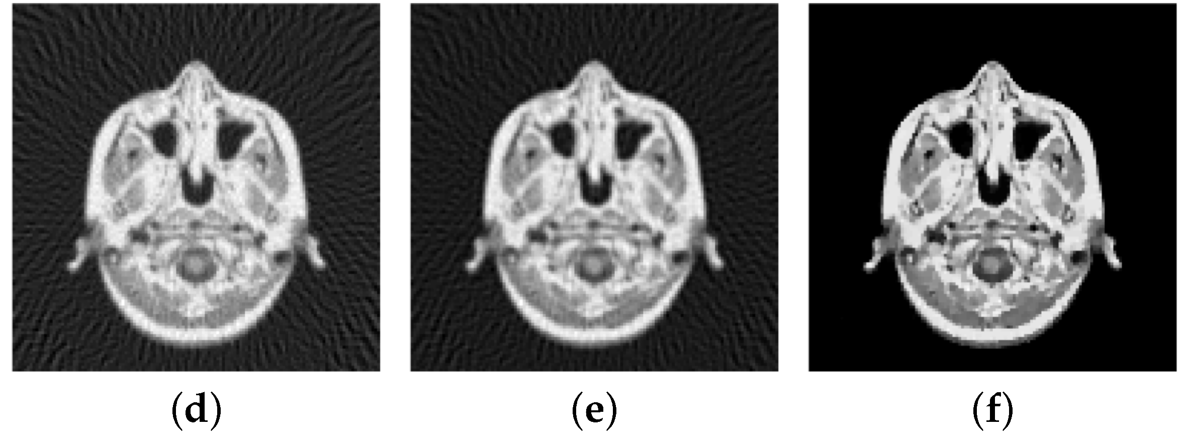
For our numerical studies we consider the images shown in Figure 1 of size 256 × 256 pixels and in Figure 2. The image intensity range of all original images considered in this paper is , i.e., and . Our proposed algorithms automatically transform this images into the dynamic range , here with . That is, let be the original image before any corruption, then . Moreover, the solution generated by the semi-smooth Newton method is afterwards back-transformed, i.e., the generated solution is transformed to . Note that is not necessarily in , except .
As a comparison for the different restoration qualities of the restored image we use the PSNR [49] (peak signal-to-noise ratio) given by
where denotes the original image before any corruption and the restored image, which is widely used as an image quality assessment measure, and the MSSIM [50] (mean structural similarity), which usually relates to perceived visual quality better than PSNR. In general, when comparing PSNR and MSSIM, large values indicate better reconstruction than small values.
In our experiments we also report on the computational time (in seconds) and the number of iterations (it) needed until the considered algorithms are terminated.
In all the following experiments the parameter is chosen to be 0 for image denoising (i.e., ), since then no additional smoothing is needed, and if (i.e., for image deblurring, image inpainting, for reconstructing from partial Fourier-data, and for reconstructing from sampled Radon-transform).
6.1. Dependency on the Parameter
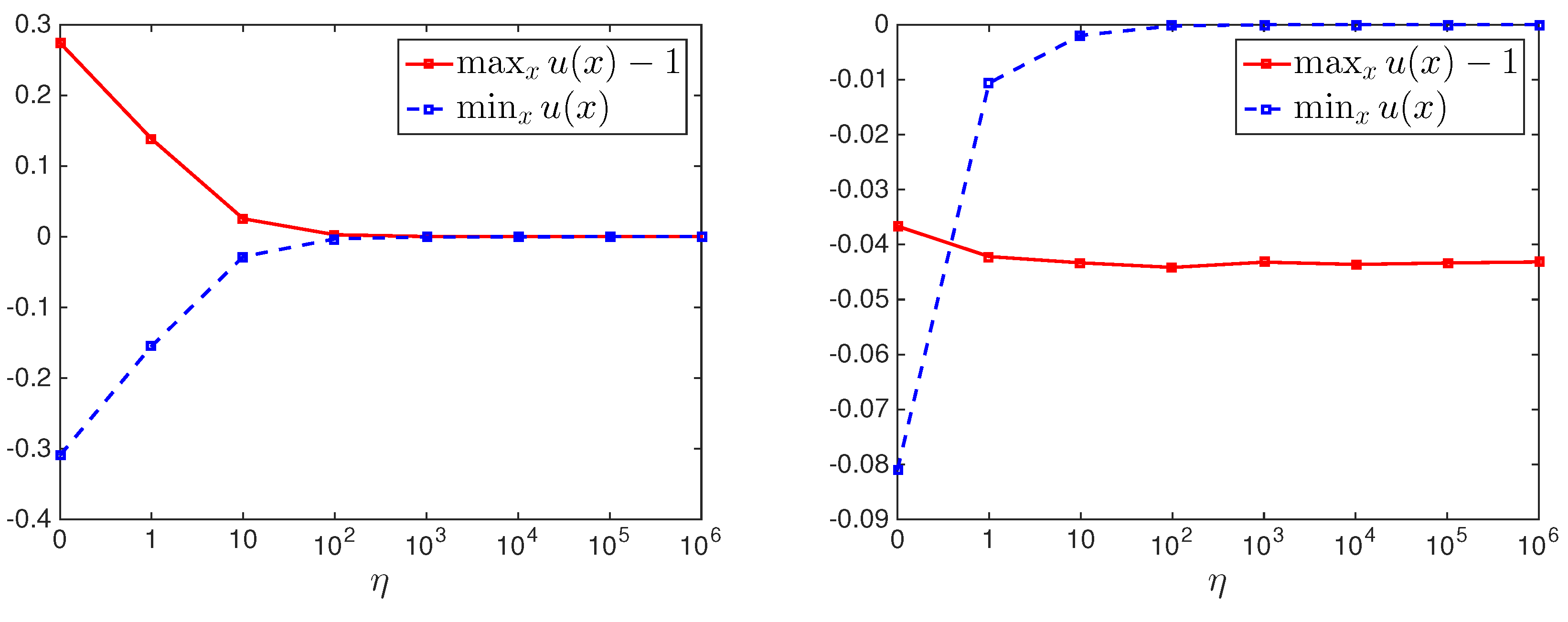
We start by investigating the influence of the parameter on the behavior of the semi-smooth Newton algorithm and its generated solution. Let us recall, that is responsible how strictly the box-constraint is adhered. In order to visualize how good the box-constraint is fulfilled for a chosen in Figure 3 we depict and with , , and u being the back-transformed solution, i.e., , where is obtained via the semi-smooth Newton method. As long as and are positive and negative, respectively, the box-constraint is not perfectly adhered. From our experiments for image denoising and image deblurring, see Figure 3, we clearly see that the larger the more strictly the box-constraint is adhered. In the rest of our experiments we choose , which seems sufficiently large to us and the box-constraint seems to hold accurately enough.
6.2. Box-Constrained Versus Non-Box-Constrained
In the rest of this section we are going to investigate how much the solution (and its restoration quality) depends on the box-constraint and if this is a matter on how the regularization parameter is chosen. We start by comparing for different values of the solutions obtained by the semi-smooth Newton method without a box-constraint (i.e., ) with the ones generated by the same algorithm with (i.e., a box-constraint is incorporated). Our obtained results are shown in Table 1 for image denoising and in Table 2 for image deblurring. We obtain, that for small we gain “much” better results with respect to PSNR and MSSIM with a box-constraint than without. The reason for this is that if no box-constraint is used and is small then nearly no regularization is performed and hence noise, which is violating the box-constraint, is still present. Therefore incorporating a box-constraint is reasonable for these choices of parameters. However, if is sufficiently large then we numerically observe that the solution of the box-constrained and non-box-constrained problem are the same. This is not surprising, because there exists such that for all the solution of problem (2) is , see [4] (Lemma 2.3). That is, for such the minimizer of problem (2) is the average of the observation which lies in the image intensity range of the original image, as long as the mean of Gaussian noise is 0 (or sufficiently small). This implies that in such a case the minimizer of problem (2) and problem (4) are equivalent. Actually this equivalency already holds if is sufficiently large such that the respective solution of problem (2) lies in the dynamic range of the original image, which is the case in our experiments for . Hence, whether it makes sense or not to incorporate a box-constraint into the considered model depends on the choice of parameters. The third and fourth value of in Table 1 and Table 2 refer to the ones which equalize problem (2) and problem (1), and respectively problem (4) and problem (3). In the sequel we call such parameters optimal, since a solution of the penalized problem also solves the related constrained problem. However, we note that these -values are in general not giving the best results with respect to PSNR and MSSIM, but they are usually close to the results with the largest PSNR and MSSIM. For both type of applications, i.e., image denoising and image deblurring, these optimal -values are nearly the same for problem (2) and problem (1), and respectively problem (4) and problem (3) and hence also the PSNR and MSSIM of the respective results are nearly the same. Nevertheless, we mention that for image deblurring the largest PSNR and MSSIM in these experiments is obtained for with a box-constraint.
In Table 3 and Table 4 we also report on an additional strategy. In this approach we threshold (or project) the observation g such that the box-constraint holds in any pixel and use then the proposed Newton method with . For large this is an inferior approach, but for small this seems to work similar to incorporating a box-constraint, at least for image denoising. However, it is outperformed by the other approaches.
6.3. Comparison with Optimal Regularization Parameters
In order to determine the optimal parameters for a range of different examples we assume that the noise-level is at hand and utilize the pAPS-algorithm presented in [36]. Alternatively, instead of computing a suitable , we may solve the constrained optimization problems (1) and (3) directly by using the alternating direction methods of multipliers (ADMM). An implementation of the ADMM for solving problem (1) is presented in [51], which we refer to as the ADMM in the sequel. For solving problem (3) a possible implementation is suggested in [27]. However, for comparison purposes we use a slightly different version, which uses the same succession of updates as the ADMM in [51], see Appendix B for a description of this version. In the sequel we refer to this algorithm as the box-contrained ADMM. We do not expect the same results for the pAPS-algorithm and the (box-contrained) ADMM, since in the pAPS-algorithm we use the semi-smooth Newton method which generates an approximate solution of problem (15), that is not equivalent to problem (1) and problem (3). In all the experiments in the pAPS-algorithm we set the initial regularization parameter to be .
6.3.1. pdN versus ADMM
We start by comparing the performance of the proposed primal-dual semi-smooth Newton method (pdN) and the ADMM. In these experiments we assume that we know the optimal parameters , which are then used in the pdN. Note, that a fair comparison of these two methods is difficult, since they are solving different optimization problems, as already mentioned above. However, we still compare them in order to understand better the performance of the algorithms in the sequel section.
The comparison is performed for image denoising and image deblurring and the respective findings are collected in Table 5 and Table 6. From there we clearly observe, that the proposed pdN with reaches in all experiments the desired reconstruction significantly faster than the box-constrained ADMM. While the number of iterations for image denoising is approximately the same for both methods, for image deblurring the box-constrained pdN needs significantly less iterations than the other method. In particular, the pdN needs nearly the same amount of iterations independently of the application. However, more iterations for small are needed. Note, that the pdN converges at a superlinear rate and hence a faster convergence than the box-constrained ADMM is not surprising but supports the theory.
6.3.2. Image Denoising
In Table 7 and Table 8 we summarize our findings for image denoising. We observe that adding a box-constraint to the considered optimization problem leads to a possibly slight improvement in PSNR and MSSIM. While in some cases there is some improvement (see for example the image “numbers”) in other examples no improvement is gained (see for example the image “barbara”). In order to make the overall improvement more visible, in the last row of Table 7 and Table 8 we add the average PSNR and MSSIM of all computed restorations. It shows that on average we may expect a gain of around 0.05 PSNR and around 0.001 MSSIM, which is nearly nothing. Moreover, we observe, that the pAPS-algorithm computes the optimal for the box-constrained problem on average faster than the one for the non-box-constrained problem. We remark, that the box-constrained version needs less (or at maximum the same amount of) iterations as the version with . The reason for this might be that in each iterations, due to the thresholding of the approximation by the box-constraint, a longer or better step towards the minimizer than by the non-box-constrained pAPS-algorithm is performed. At the same time also the reconstructions of the box-constrained pAPS-algorithm yield higher PSNR and MSSIM than the ones obtained by the pAPS-algorithm with . The situation seems to be different for the ADMM. On average, the box-constrained ADMM and the (non-box-constrained) ADMM need approximately the same run-time.
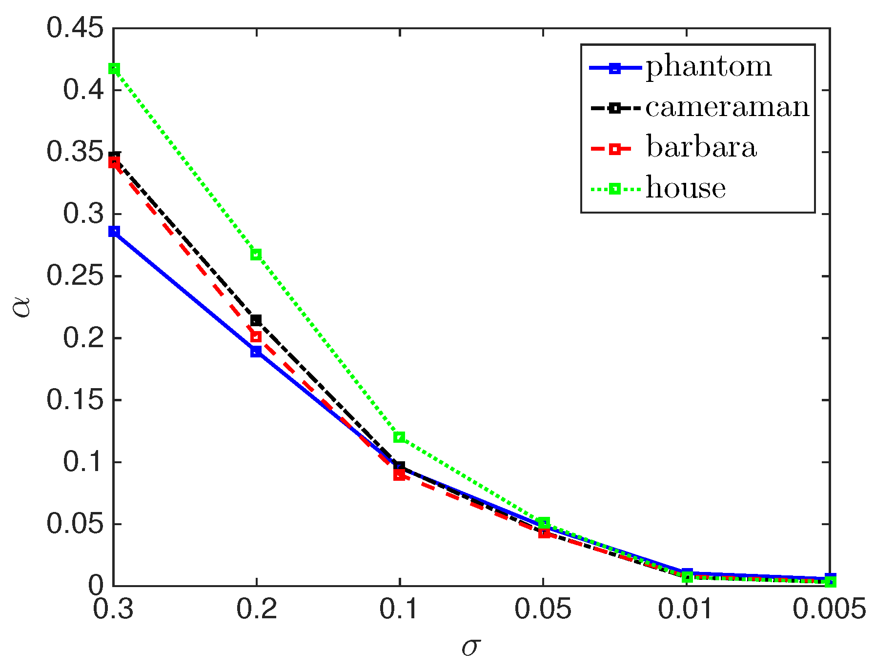
For several examples (i.e., the images “phantom”, “cameraman”, “barbara”, “house”) the choice of the regularization parameter by the box-constrained pAPS-algorithm with respect to the noise-level is depicted in Figure 4. Clearly, the parameter is selected to be smaller the less noise is present in the image.
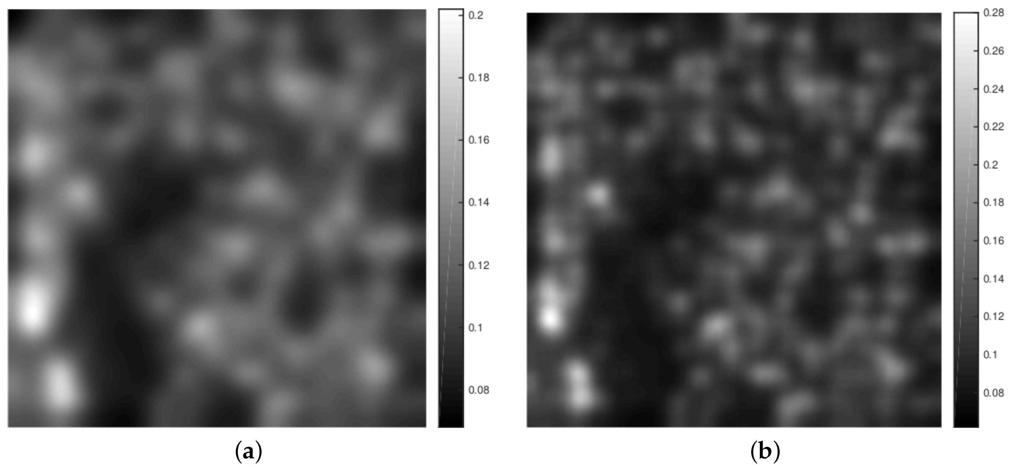
We are now wondering whether a box-constraint is more important when the regularization parameter is non-scalar, i.e., when is a function. For computing suitable locally varying we use the pLATV-algorithm proposed in [36], whereby we set in all considered examples the initial (non-scalar) regularization parameter to be constant . Note, that the continuity assumption on in problem (5) and problem (6) is not needed in our discrete setting, since is well defined for any . We approximate such for problem (20) with (unconstrained) and with (box-constrained) and obtain also here that the gain with respect to PSNR and MSSIM is of the same order as in the scalar case, see Table 9.
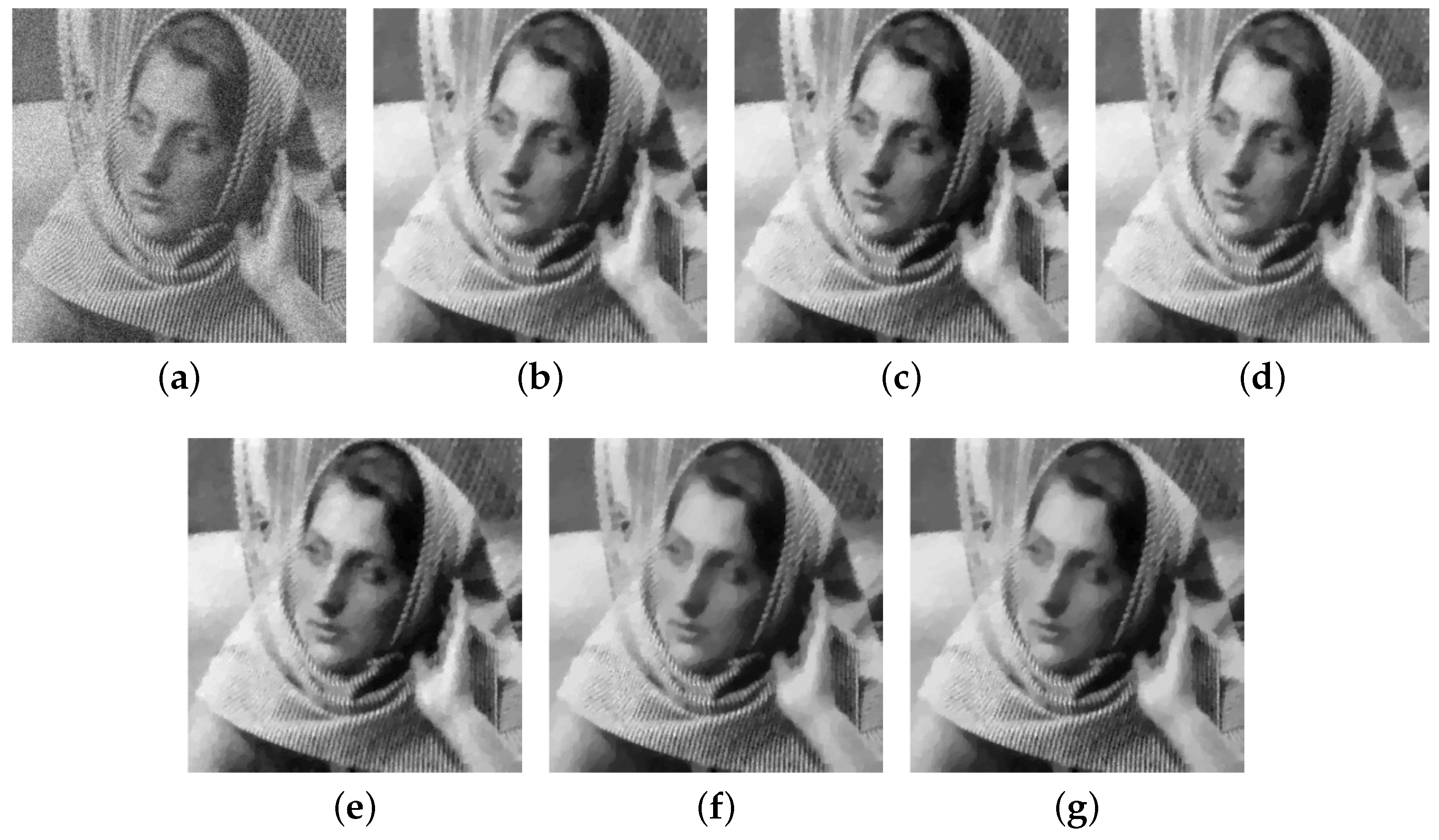
For and the image “barbara” we show in Figure 5 the reconstructions generated by the considered algorithms. As indicated by the quality measures, all the reconstructions look nearly alike, whereby in the reconstructions produced by the pLATV-algorithm details, like the pattern of the scarf, are (slightly) better preserved. The spatially varying of the pLATV-algorithm is depicted in Figure 6. There we clearly see, that at the scarf around the neck and shoulder the values of are small, allowing to preserve the details better.
6.3.3. Image Deblurring
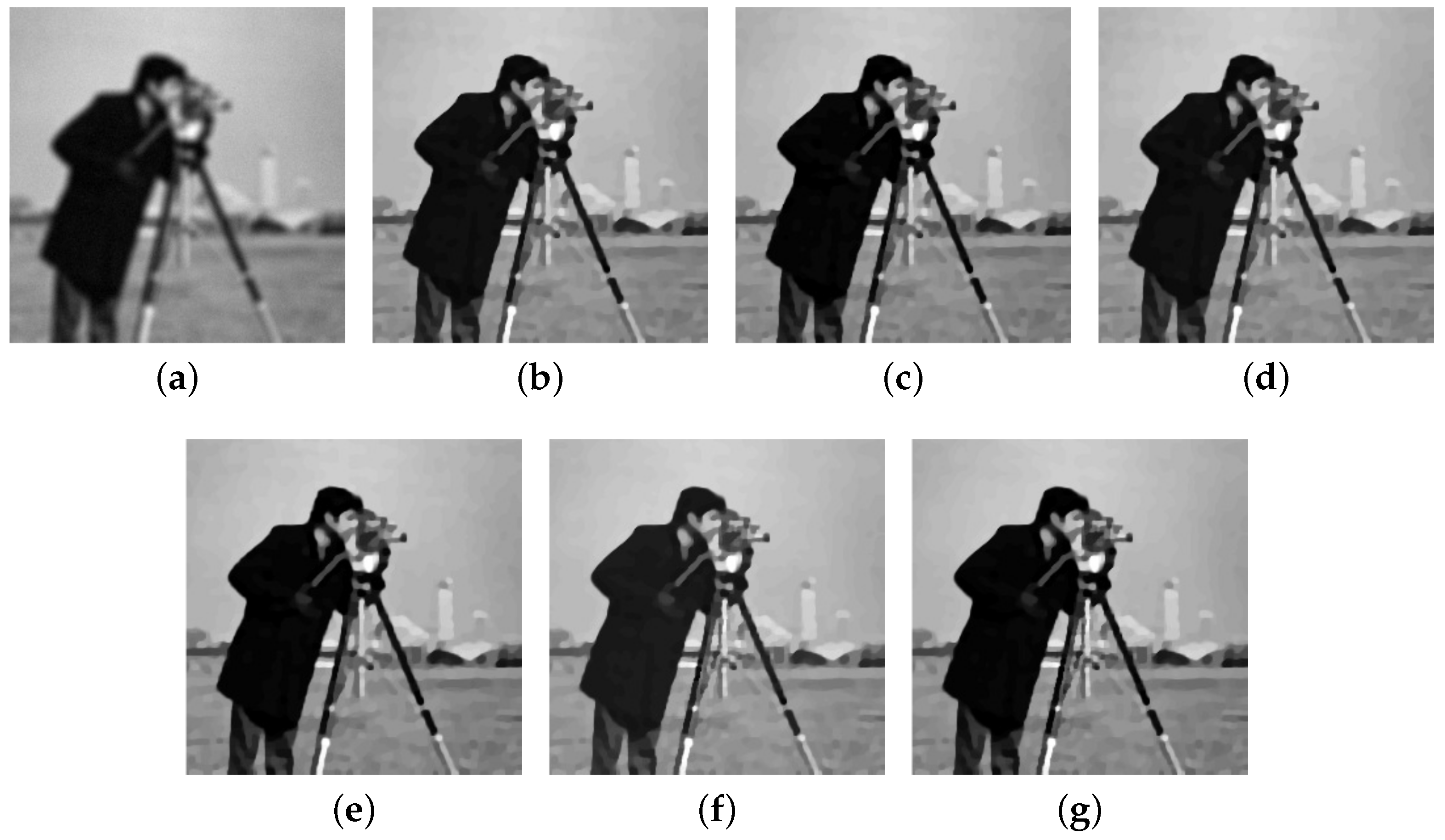
Now we consider the images in Figure 1a–c, convolve them first with a Gaussian kernel of size and standard deviation 3 and then add some Gaussian noise with mean 0 and standard deviation . Here we again compare the results obtained by the pAPS-algorithm, the ADMM, and the pLATV-algorithm for the box-constrained and non-box-constrained problems. Our findings are summarized in Table 10. Also here we observe a slight improvement with a box-constraint with respect to PSNR and MSSIM. The choice of the regularization parameters by the box-constrained pAPS-algorithm is depicted in Figure 7. In Figure 8 we present for the image “cameraman” and the reconstructions produced by the respective methods. Also here, as indicated by the quality measures, all the restorations look nearly the same. The locally varying generated by the pLATV-algorithm are depicted in Figure 9.
6.3.4. Image Inpainting
The problem of filling in and recovering missing parts in an image is called image inpainting. We call the missing parts inpainting domain and denote it by . The linear bounded operator K is then a multiplier, i.e., , where is the indicator function of . Note, that K is not injective and hence is not invertible. Hence in this experiment we need to set so that we can use the proposed primal-dual semismooth Newton method. In particular, as mentioned above, we choose .
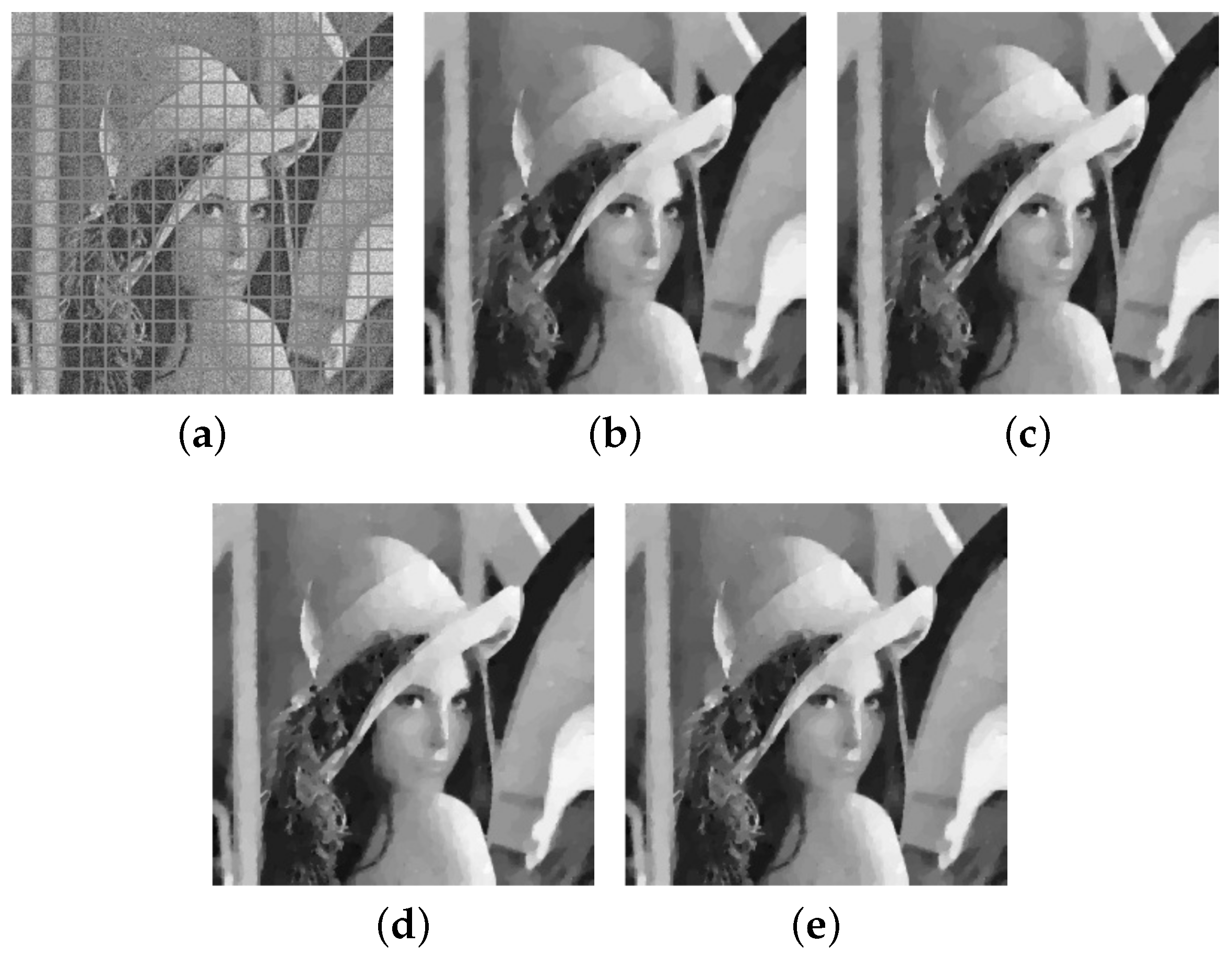
In the considered experiments the inpainting domain are gray bars as shown in Figure 10a, where additionally additive white Gaussian noise with is present. In particular, we consider examples with . The performance of the pAPS- and pLATV-algorithm with and without a box-constraint reconstructing the considered examples are summarized in Table 11 and Table 12. We observe, that adding a box-constraint does not seem to change the restoration considerably. However, as in the case of image denoising, the pAPS-algorithm with box-constrained pdN needs less iterations and hence less time than the same algorithm without a box-constraint to reach the stopping criterion. Figure 10 shows a particular example for image inpainting and denoising with . It demonstrates that visually there is nearly no difference between the restoration obtained by the considered approaches. Moreover, we observe that the pLATV-algorithm seems to be not suited to the task of image inpainting. A reason for this might be, that the pLATV-algorithm does not take the inpainting domain correctly into account. This is visible in Figure 11 where the spatially varying seems to be chosen small in the inpainting domain, which not necessarily seems to be a suitable choice.
6.3.5. Reconstruction from Partial Fourier-Data
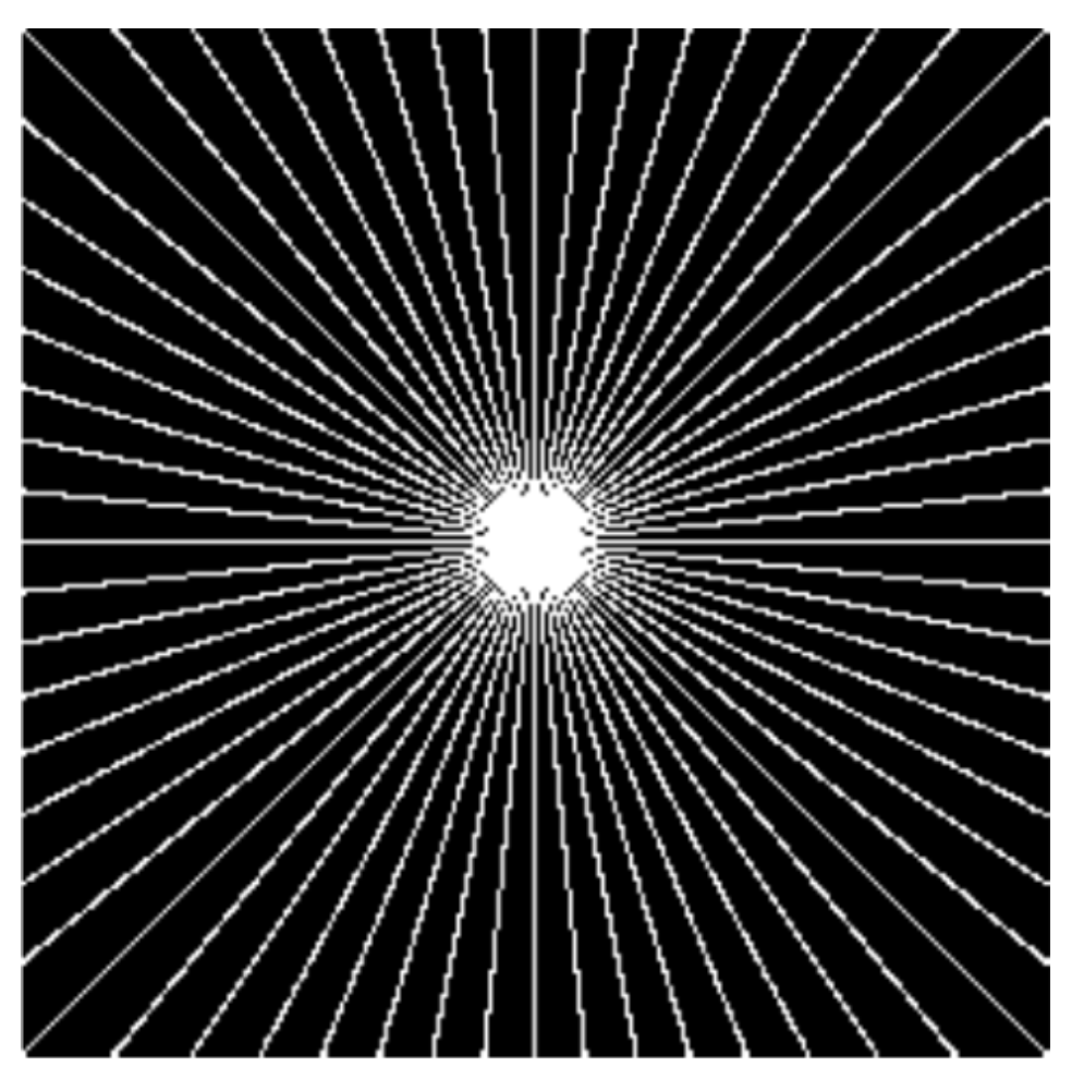
In magnetic resonance imaging one wishes to reconstruct an image which is only given by partial Fourier data and additionally distorted by some additive Gaussian noise with zero mean and standard deviation . Hence, the linear bounded operator is , where is the Fourier matrix and S is a downsampling operator which selects only a few output frequencies. The frequencies are usually sampled along radial lines in the frequency domain, in particular in our experiments along 32 radial lines, as visualized in Figure 12.
In our experiments we consider the images of Figure 2, transformed to its Fourier frequencies. As already mentioned, we sample the frequencies along 32 radial lines and add some Gaussian noise with zero mean and standard deviation . In particular, we consider different noise-levels, i.e., . We reconstruct the obtained data via the pAPS- and pLATV-algorithm by using the semi-smooth Newton method first with (no box-constraint) and then with (with box-constraint). In Table 13 we collect our findings. We observe that the pLATV-algorithm seems not to be suitable for this task, since it is generating inferior results. For scalar we observe as before, that a slight improvement with respect to PSNR and MSSIM is expectable when a box-constraint is used. In Figure 13 we present the reconstructions generated by the considered algorithms for a particular example, demonstrating the visual behavior of the methods.
6.3.6. Reconstruction from Sampled Radon-Data
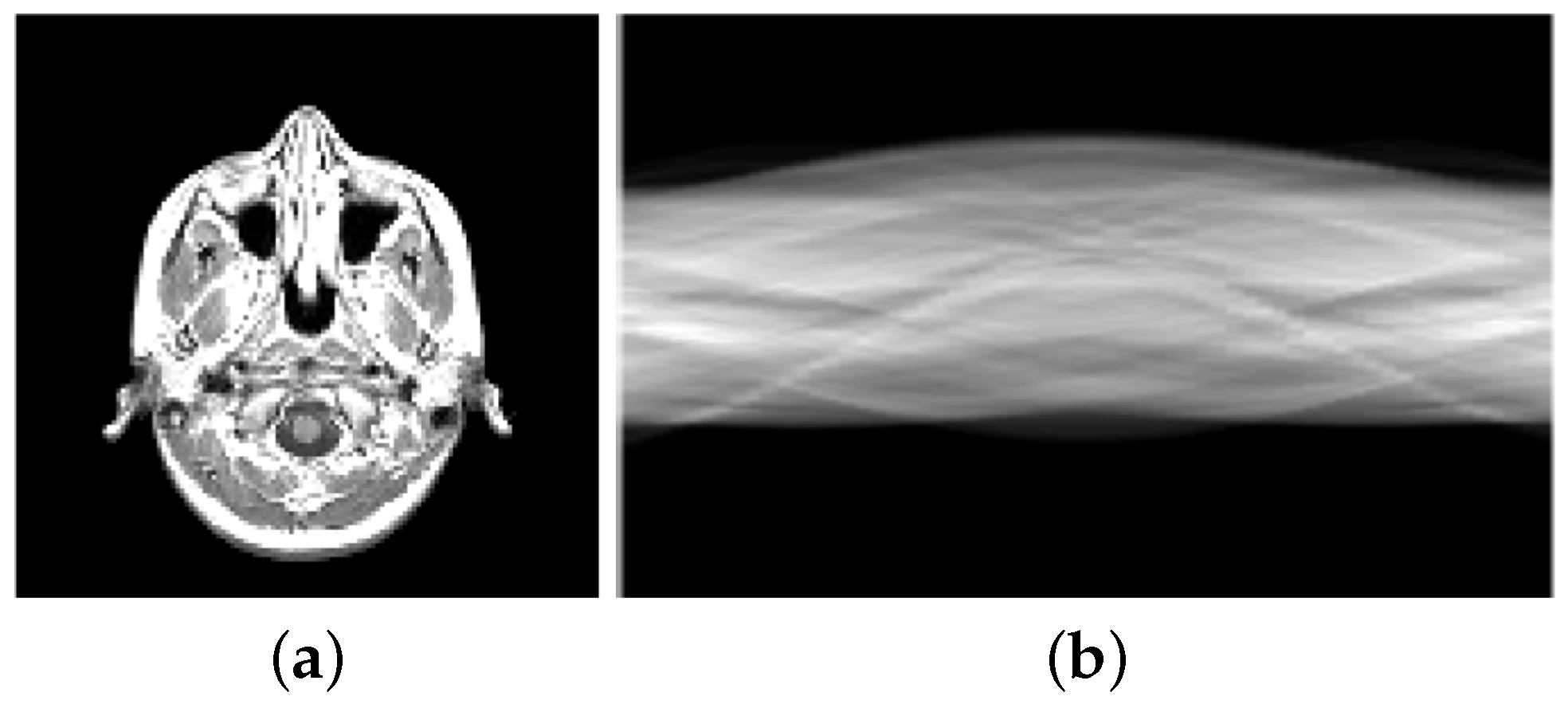
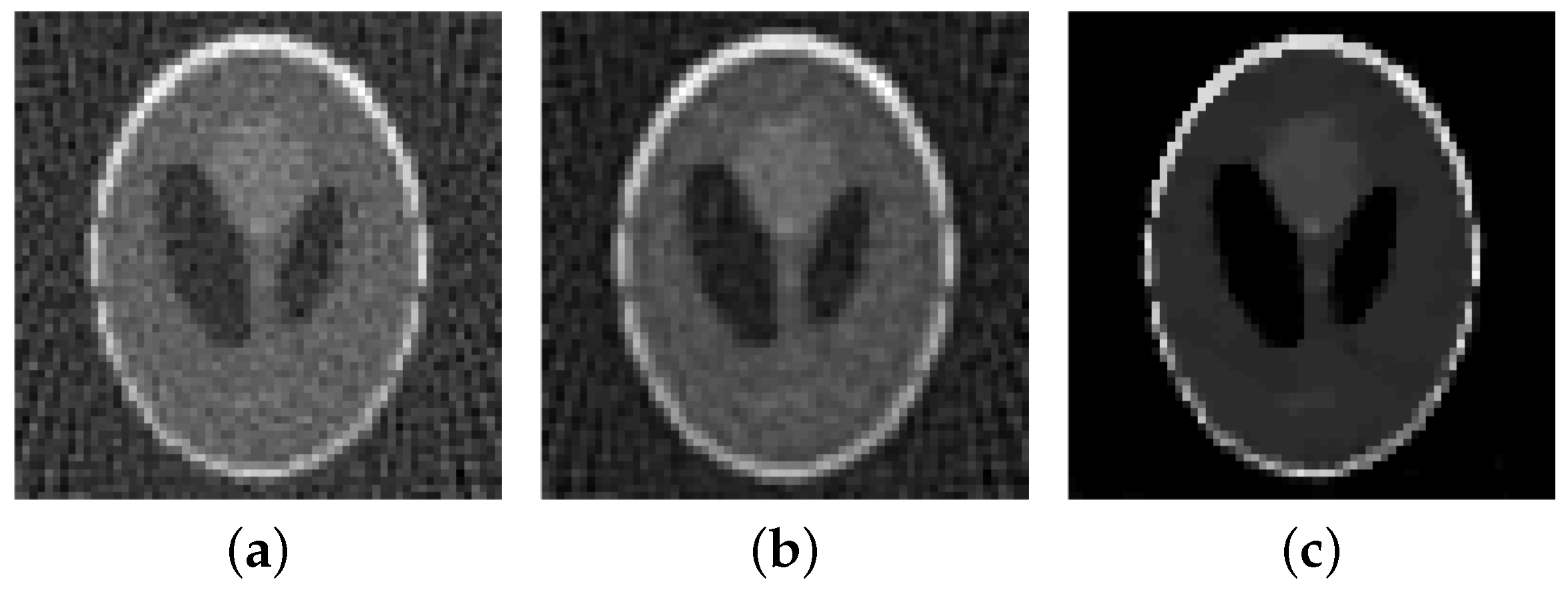
In computerized tomography instead of a Fourier-transform a Radon-transform is used in order to obtain a visual image from the measured physical data. Also here the data is obtained along radial lines. Here we consider the Shepp-Logan phantom, see Figure 14a, and a slice of a body, see Figure 15a. The sinogram in Figure 14a and Figure 15b are obtained by sampling along 30 and 60 radial lines, respectively, Note, that the sinogram is in general noisy. Here the data is corrupted by Gaussian white noise with standard deviation , whereby for the data of the Shepp-Logan phantom and for the data of the slice of the head. Using the inverse Radon-transform we obtain Figure 16a,b, which is obviously a suboptimal reconstruction. A more sophisticated approach utilizes the -TV model which yields the reconstruction depicted in Figure 16b,e, where we use the pAPS-algorithm and the proposed primal-dual algorithm with . However, since an image can be assumed to have non-negative values, we may incorporate a non-negativity constraint via the box-constrained -TV model yielding the result in Figure 16c,f, which is a much better reconstruction. Also here the parameter is automatically computed by the pAPS-algorithm and the non-negativity constraint is incorporated by setting in the semi-smooth Newton method. In order to compute the Radon-matrix in our experiments we used the FlexBox [52].
Other applications where a box-constraint, and in particular a non-negativity improves the image reconstruction quality significantly include for example magnetic particle imaging, see for example [53] and references therein.
7. Automated Parameter Selection
We recall, that if the noise-level is not known, then the problems (1) and (3) cannot be considered. Moreover, the selection of the parameter in problem (2) cannot be achieved by using the pAPS-algorithm, since this algorithm is based on problem (1). Note, that also other methods, like the unbiased predictive risk estimator method (UPRE) [54,55] and approaches based on the Stein unbiased risk estimator method (SURE) [56,57,58,59,60] use knowledge of the noise-level and hence cannot be used for selecting a suitable parameter if is unknown.
If we assume that is unknown but the image intensity range of the original image is known, i.e., , then we may use this information for choosing the parameter in problem (2). This may be performed by applying the following algorithm:
| Box-constrained automatic parameter selection (bcAPS): Initialize (sufficiently small) and set 1. Solve . 2. If increase (i.e., with ), else STOP. 3. Set and continue with step 1. |
Here is an arbitrary parameter chosen manually such that the generated restoration u is not over-smoothed, i.e., there exist such that and/or . In our experiments it turned out that seems to be a reasonable choice, so that the generated solution has the wished property.
Numerical Examples
In our experiments the minimization problem in step 1 of the bcAPS algorithm is approximately solved by the proposed primal-dual semi-smooth Newton method with . We set the initial regularization parameter for image denoising and for image deblurring. Moreover, we set in the bcAPS-algorithm to increase the regularization parameter.
Experiments for image denoising, see Table 14, show that the bcAPS-algorithm finds suitable parameters in the sense that the PSNR and MSSIM of these reconstructions is similar to the ones obtained with the pAPS-algorithm (when is known); also compare with Table 7 and Table 10. This is explained by the observation that also the regularization parameters calculated by the bcAPS-algorithm do not differ much from the ones obtained via the pAPS-algorithm. For image deblurring, see Table 15, the situation is not so persuasive. In particular, the obtained regularization parameter of the two considered methods differ more significantly than before, resulting in different PSNR and MSSIM. However, in the case the considered quality measures of the generated reconstructions are nearly the same.
We also remark, that in all the experiments the pAPS-algorithm generated reconstructions, which have larger PSNR and MSSIM than the ones obtained by the bcAPS-algorithm. From this observation it seems more useful to know the noise-level than the image intensity range. However, if the noise-level is unknown but the image intensity is known, then the bcAPS-algorithm may be a suitable choice.
8. Conclusions
In this work we investigated the quality of restored images when the image intensity range of the original image is additionally incorporated into the -TV model as a box-constraint. We observe that this box-constraint may indeed improve the quality of reconstructions. However, if the observation already fulfills the box-constraint, then it clearly does not change the solution at all. Moreover, in a lot of applications the proper choice of the regularization parameter seems much more important than an additional box-constraint. Nevertheless, also then a box-constraint may improve the quality of the restored image, although the improvement is then only very little. On the contrary the additional box-constraint may improve the computational time significantly. In particular, for image deblurring and in magnetic resonance imaging using the pAPS-algorithm the computational time is about doubled, while the quality of the restoration is basically not improved. This suggests, that for these applications an additional box-constraint may not be reasonable. Note, that the run-time of the ADMM is independent whether a box-constraint is used or not.
For certain applications, as in computerized tomography, a box-constraint (in particular a non-negativity constraint) improves the reconstruction considerably. Hence, the question rises under which conditions an additional box-constraint indeed has significant influence on the reconstruction when the present parameters are chosen in a nearly optimal way.
If the noise-level of an corrupted image is unknown but the image intensity range of the original image is at hand, then the image intensity range may be used to calculate a suitable regularization parameter . This can be done as explained in Section 7. Potential future research may consider different approaches, as for example in an optimal control setting. Then one may want to solve
where and J is a suitable functional, cf. [61,62,63] for other optimal control approaches in image reconstruction.
Conflicts of Interest
The author declares no conflict of interest.
Appendix A. Proof of Proposition 3
In order to compute the Fenchel dual of problem (14) we set ,
with and .
By the definition of conjugate we have
Then u is a supremum if
which implies . Hence
In order to compute the conjugate we split into two functionals and defined as
whereas . We have, that
A function is a supremum of this set if
with . The equality implies from which we deduce
For the conjugate of we get
Hence is a supremum if
Thus
From (A1) we obtain that
Using this observation yields
By the Fenchel duality theorem the assertion follows.
Appendix B. Box-Constrained ADMM
In [51] an ADMM for solving the constrained problem (1) in a finite dimensional setting is presented. In a similar way we may solve the discrete version of problem (3), i.e.,
where we use the notation of Section 5 and with being a circular matrix and as in [51]. Moreover, , refers to the standard definition of the -norm, i.e, , and denotes the inner product.
The augmented Lagrangian of this problem is
with , , , and denoting the penalty parameter. Hence the ADM for solving problem (A2) runs as follows:
Box-constrained ADMM: Initialize , and set ;
|
In order to obtain in step (1) a linear system that may be diagonalized by the DFT is to solve. The solution of the minimization problem in step (2) might be computed as described in [51] (Section 4.2). More precisely, we have
where is called proximal operator of f. If we write , we can decompose as
From [51] we know, that
and is a projection onto a weighted -ball, which might be implemented as described in [64]. From the definition of the proximal operator we see that
is just the simple orthogonal projection of onto .
References
- Rudin, L.I.; Osher, S.; Fatemi, E. Nonlinear total variation based noise removal algorithms. Phys. D 1992, 60, 259–268. [Google Scholar] [CrossRef]
- Ambrosio, L.; Fusco, N.; Pallara, D. Functions of Bounded Variation and Free Discontinuity Problems; Oxford Mathematical Monographs, The Clarendon Press, Oxford University Press: New York, NY, USA, 2000; pp. xviii+434. [Google Scholar]
- Giusti, E. Minimal Surfaces and Functions of Bounded Variation; Vol. 80—Monographs in Mathematics; Birkhäuser Verlag: Basel, Switzerland, 1984; pp. xii+240. [Google Scholar]
- Chambolle, A.; Lions, P.L. Image recovery via total variation minimization and related problems. Numer. Math. 1997, 76, 167–188. [Google Scholar] [CrossRef]
- Beck, A.; Teboulle, M. Fast gradient-based algorithms for constrained total variation image denoising and deblurring problems. IEEE Trans. Image Process. 2009, 18, 2419–2434. [Google Scholar] [CrossRef] [PubMed]
- Boţ, R.I.; Hendrich, C. A Douglas–Rachford type primal-dual method for solving inclusions with mixtures of composite and parallel-sum type monotone operators. SIAM J. Optim. 2013, 23, 2541–2565. [Google Scholar] [CrossRef]
- Boţ, R.I.; Hendrich, C. Convergence analysis for a primal-dual monotone+ skew splitting algorithm with applications to total variation minimization. J. Math. Imaging Vis. 2014, 49, 551–568. [Google Scholar] [CrossRef]
- Burger, M.; Sawatzky, A.; Steidl, G. First order algorithms in variational image processing. In Splitting Methods in Communication, Imaging, Science, and Engineering; Springer: Cham, Switzerland, 2014; pp. 345–407. [Google Scholar]
- Chambolle, A. An algorithm for total variation minimization and applications. J. Math. Imaging Vis. 2004, 20, 89–97. [Google Scholar]
- Chambolle, A.; Pock, T. A first-order primal-dual algorithm for convex problems with applications to imaging. J. Math. Imaging Vis. 2011, 40, 120–145. [Google Scholar] [CrossRef]
- Chan, T.F.; Golub, G.H.; Mulet, P. A nonlinear primal-dual method for total variation-based image restoration. SIAM J. Sci. Comput. 1999, 20, 1964–1977. [Google Scholar] [CrossRef]
- Combettes, P.L.; Vũ, B.C. Variable metric forward–backward splitting with applications to monotone inclusions in duality. Optimization 2014, 63, 1289–1318. [Google Scholar] [CrossRef]
- Combettes, P.L.; Wajs, V.R. Signal recovery by proximal forward-backward splitting. Multiscale Model. Simul. 2005, 4, 1168–1200. [Google Scholar] [CrossRef]
- Condat, L. A primal–dual splitting method for convex optimization involving Lipschitzian, proximable and linear composite terms. J. Optim. Theory Appl. 2013, 158, 460–479. [Google Scholar] [CrossRef] [Green Version]
- Darbon, J.; Sigelle, M. A fast and exact algorithm for total variation minimization. In Pattern Recognition and Image Analysis; Springer: Berlin/Heidelberg, Germany, 2005; pp. 351–359. [Google Scholar]
- Darbon, J.; Sigelle, M. Image restoration with discrete constrained total variation. I. Fast and exact optimization. J. Math. Imaging Vis. 2006, 26, 261–276. [Google Scholar] [CrossRef]
- Daubechies, I.; Teschke, G.; Vese, L. Iteratively solving linear inverse problems under general convex constraints. Inverse Probl. Imaging 2007, 1, 29–46. [Google Scholar] [CrossRef]
- Dobson, D.C.; Vogel, C.R. Convergence of an iterative method for total variation denoising. SIAM J. Numer. Anal. 1997, 34, 1779–1791. [Google Scholar] [CrossRef]
- Goldstein, T.; Osher, S. The split Bregman method for L1-regularized problems. SIAM J. Imaging Sci. 2009, 2, 323–343. [Google Scholar] [CrossRef]
- Hintermüller, M.; Kunisch, K. Total bounded variation regularization as a bilaterally constrained optimization problem. SIAM J. Appl. Math. 2004, 64, 1311–1333. [Google Scholar]
- Hintermüller, M.; Stadler, G. An infeasible primal-dual algorithm for total bounded variation-based inf-convolution-type image restoration. SIAM J. Sci. Comput. 2006, 28, 1–23. [Google Scholar] [CrossRef]
- Nesterov, Y. Smooth minimization of non-smooth functions. Math. Program. 2005, 103, 127–152. [Google Scholar] [CrossRef]
- Osher, S.; Burger, M.; Goldfarb, D.; Xu, J.; Yin, W. An iterative regularization method for total variation-based image restoration. Multiscale Model. Simul. 2005, 4, 460–489. [Google Scholar] [CrossRef]
- Alliney, S. A property of the minimum vectors of a regularizing functional defined by means of the absolute norm. IEEE Trans. Signal Process. 1997, 45, 913–917. [Google Scholar] [CrossRef]
- Nikolova, M. Minimizers of cost-functions involving nonsmooth data-fidelity terms. Application to the processing of outliers. SIAM J. Numer. Anal. 2002, 40, 965–994. [Google Scholar] [CrossRef]
- Nikolova, M. A variational approach to remove outliers and impulse noise. J. Math. Imaging Vis. 2004, 20, 99–120. [Google Scholar] [CrossRef]
- Chan, R.H.; Tao, M.; Yuan, X. Constrained total variation deblurring models and fast algorithms based on alternating direction method of multipliers. SIAM J. Imaging Sci. 2013, 6, 680–697. [Google Scholar] [CrossRef]
- Ma, L.; Ng, M.; Yu, J.; Zeng, T. Efficient box-constrained TV-type-l1 algorithms for restoring images with impulse noise. J. Comput. Math. 2013, 31, 249–270. [Google Scholar] [CrossRef]
- Morini, B.; Porcelli, M.; Chan, R.H. A reduced Newton method for constrained linear least-squares problems. J. Comput. Appl. Math. 2010, 233, 2200–2212. [Google Scholar] [CrossRef]
- Gabay, D.; Mercier, B. A dual algorithm for the solution of nonlinear variational problems via finite element approximation. Comput. Math. Appl. 1976, 2, 17–40. [Google Scholar] [CrossRef]
- Williams, B.M.; Chen, K.; Harding, S.P. A new constrained total variational deblurring model and its fast algorithm. Numer. Algorithms 2015, 69, 415–441. [Google Scholar] [CrossRef]
- Liu, R.W.; Shi, L.; Yu, S.C.H.; Wang, D. Box-constrained second-order total generalized variation minimization with a combined L1,2 data-fidelity term for image reconstruction. J. Electron. Imaging 2015, 24, 033026. [Google Scholar] [CrossRef]
- Hintermüller, M.; Langer, A. Subspace correction methods for a class of nonsmooth and nonadditive convex variational problems with mixed L1/L2 data-fidelity in image processing. SIAM J. Imaging Sci. 2013, 6, 2134–2173. [Google Scholar] [CrossRef]
- Bardsley, J.M.; Vogel, C.R. A nonnegatively constrained convex programming method for image reconstruction. SIAM J. Sci. Comput. 2004, 25, 1326–1343. [Google Scholar] [CrossRef]
- Vogel, C.R. Computational Methods for Inverse Problems; Society for Industrial and Applied Mathematics (SIAM): Philadelphia, PA, USA, 2002; Volume 23. [Google Scholar]
- Langer, A. Automated Parameter Selection for Total Variation Minimization in Image Restoration. J. Math. Imaging Vis. 2017, 57, 239–268. [Google Scholar] [CrossRef]
- Dong, Y.; Hintermüller, M.; Neri, M. An efficient primal-dual method for L1 TV image restoration. SIAM J. Imaging Sci. 2009, 2, 1168–1189. [Google Scholar] [CrossRef]
- Dong, Y.; Hintermüller, M.; Rincon-Camacho, M.M. Automated regularization parameter selection in multi-scale total variation models for image restoration. J. Math. Imaging Vis. 2011, 40, 82–104. [Google Scholar] [CrossRef]
- Hintermüller, M.; Rincon-Camacho, M.M. Expected absolute value estimators for a spatially adapted regularization parameter choice rule in L1-TV-based image restoration. Inverse Probl. 2010, 26, 085005. [Google Scholar] [CrossRef]
- Cao, V.C.; Reyes, J.C.D.L.; Schönlieb, C.B. Learning optimal spatially-dependent regularization parameters in total variation image restoration. Inverse Probl. 2017, 33, 074005. [Google Scholar]
- Langer, A. Locally adaptive total variation for removing mixed Gaussian-impulse noise. 2017; submitted. [Google Scholar]
- Attouch, H.; Buttazzo, G.; Michaille, G. Variational Analysis in Sobolev and BV Spaces: Applications to PDEs and Optimization, 2nd ed.; MOS-SIAM Series on Optimization; Society for Industrial and Applied Mathematics (SIAM): Philadelphia, PA, USA; Mathematical Optimization Society: Philadelphia, PA, USA, 2014; pp. xii+793. [Google Scholar]
- Ekeland, I.; Témam, R. Convex Analysis and Variational Problems, English ed.; Vol. 28—Classics in Applied Mathematics; Society for Industrial and Applied Mathematics (SIAM): Philadelphia, PA, USA, 1999; pp. xiv+402. [Google Scholar]
- Alkämper, M.; Langer, A. Using DUNE-ACFEM for Non-smooth Minimization of Bounded Variation Functions. Arch. Numer. Softw. 2017, 5, 3–19. [Google Scholar]
- Langer, A. Automated parameter selection in the L1-L2-TV model for removing Gaussian plus impulse noise. Inverse Probl. 2017, 33, 074002. [Google Scholar] [CrossRef]
- Chan, R.H.; Ho, C.W.; Nikolova, M. Salt-and-pepper noise removal by median-type noise detectors and detail-preserving regularization. IEEE Trans. Image Process. 2005, 14, 1479–1485. [Google Scholar] [CrossRef] [PubMed]
- Bartels, S. Numerical Methods for Nonlinear Partial Differential Equations; Springer: Cham, Switzerland, 2015; Volume 14. [Google Scholar]
- Ito, K.; Kunisch, K. An active set strategy based on the augmented Lagrangian formulation for image restoration. ESAIM 1999, 33, 1–21. [Google Scholar] [CrossRef]
- Bovik, A.C. Handbook of Image and Video Processing; Academic Press: Cambridge, MA, USA, 2010. [Google Scholar]
- Wang, Z.; Bovik, A.C.; Sheikh, H.R.; Simoncelli, E.P. Image quality assessment: From error visibility to structural similarity. IEEE Trans. Image Process. 2004, 13, 600–612. [Google Scholar] [CrossRef] [PubMed]
- Ng, M.K.; Weiss, P.; Yuan, X. Solving constrained total-variation image restoration and reconstruction problems via alternating direction methods. SIAM J. Sci. Comput. 2010, 32, 2710–2736. [Google Scholar] [CrossRef]
- Dirks, H. A Flexible Primal-Dual Toolbox. ArXiv E-Prints, 2016; arXiv:1603.05835. [Google Scholar]
- Storath, M.; Brandt, C.; Hofmann, M.; Knopp, T.; Salamon, J.; Weber, A.; Weinmann, A. Edge preserving and noise reducing reconstruction for magnetic particle imaging. IEEE Trans. Med. Imaging 2017, 36, 74–85. [Google Scholar] [CrossRef] [PubMed]
- Lin, Y.; Wohlberg, B.; Guo, H. UPRE method for total variation parameter selection. Signal Process. 2010, 90, 2546–2551. [Google Scholar] [CrossRef]
- Mallows, C.L. Some comments on CP. Technometrics 1973, 15, 661–675. [Google Scholar]
- Blu, T.; Luisier, F. The SURE-LET approach to image denoising. IEEE Trans. Image Process. 2007, 16, 2778–2786. [Google Scholar] [CrossRef] [PubMed]
- Donoho, D.L.; Johnstone, I.M. Adapting to unknown smoothness via wavelet shrinkage. J. Am. Stat. Assoc. 1995, 90, 1200–1224. [Google Scholar] [CrossRef]
- Deledalle, C.A.; Vaiter, S.; Fadili, J.; Peyré, G. Stein Unbiased GrAdient estimator of the Risk (SUGAR) for multiple parameter selection. SIAM J. Imaging Sci. 2014, 7, 2448–2487. [Google Scholar] [CrossRef]
- Eldar, Y.C. Generalized SURE for exponential families: Applications to regularization. IEEE Trans. Signal Process. 2009, 57, 471–481. [Google Scholar] [CrossRef]
- Giryes, R.; Elad, M.; Eldar, Y.C. The projected GSURE for automatic parameter tuning in iterative shrinkage methods. Appl. Comput. Harmon. Anal. 2011, 30, 407–422. [Google Scholar] [CrossRef]
- De los Reyes, J.C.; Schönlieb, C.B. Image denoising: Learning the noise model via nonsmooth PDE-constrained optimization. Inverse Probl. Imaging 2013, 7, 1183–1214. [Google Scholar] [CrossRef]
- Hintermüller, M.; Rautenberg, C.; Wu, T.; Langer, A. Optimal Selection of the Regularization Function in a Generalized Total Variation Model. Part II: Algorithm, its Analysis and Numerical Tests. J. Math. Imaging Vis. 2017, 59, 515–533. [Google Scholar] [CrossRef]
- Kunisch, K.; Pock, T. A bilevel optimization approach for parameter learning in variational models. SIAM J. Imaging Sci. 2013, 6, 938–983. [Google Scholar] [CrossRef]
- Weiss, P.; Blanc-Féraud, L.; Aubert, G. Efficient schemes for total variation minimization under constraints in image processing. SIAM J. Sci. Comput. 2009, 31, 2047–2080. [Google Scholar] [CrossRef]
- Boyd, S.; Parikh, N.; Chu, E.; Peleato, B.; Eckstein, J. Distributed optimization and statistical learning via the alternating direction method of multipliers. Found. Trends Mach. Learn. 2011, 3, 1–122. [Google Scholar] [CrossRef]
- Glowinski, R. Numerical Methods for Nonlinear Variational Problems; Springer: New York, NY, USA, 1984. [Google Scholar]
Figure 1.
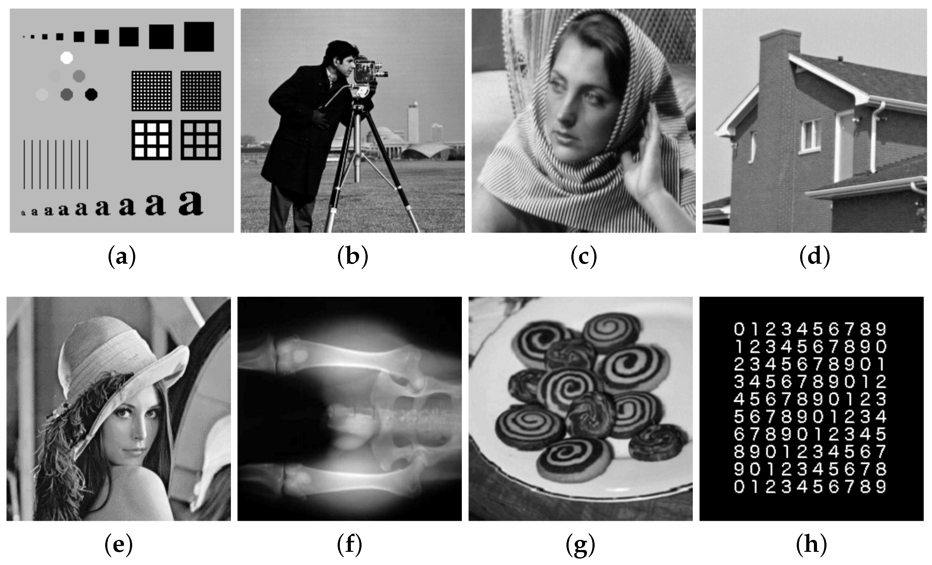
Original images of size . (a) Phantom; (b) Cameraman; (c) Barbara; (d) House; (e) Lena; (f) Bones; (g) Cookies; (h) Numbers.
Figure 1.
Original images of size . (a) Phantom; (b) Cameraman; (c) Barbara; (d) House; (e) Lena; (f) Bones; (g) Cookies; (h) Numbers.

Figure 2.
Original images (a) Shepp-Logan phantom of size pixels (b) knee of size pixels (c) slice of a human brain of size pixels.
Figure 2.
Original images (a) Shepp-Logan phantom of size pixels (b) knee of size pixels (c) slice of a human brain of size pixels.
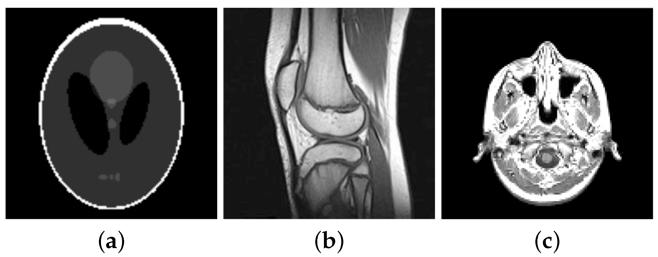
Figure 3.
Reconstruction of the cameraman image corrupted by Gaussian white noise with (left), corrupted by blurring and Gaussian white noise with (right) via the semi-smooth Newton method with for different values .
Figure 3.
Reconstruction of the cameraman image corrupted by Gaussian white noise with (left), corrupted by blurring and Gaussian white noise with (right) via the semi-smooth Newton method with for different values .

Figure 4.
Regularization parameter versus noise-level for the box-constrained pAPS in image denoising.
Figure 4.
Regularization parameter versus noise-level for the box-constrained pAPS in image denoising.

Figure 5.
Reconstruction from blurry and noisy data. (a) Noisy observation; (b) pAPS with pdN with (PSNR: 24.241; MSSIM: 0.58555); (c) pAPS with box-constrained pdN (PSNR: 24.241; MSSIM: 0.58564); (d) ADMM (PSNR: 24.224; MSSIM: 0.5883); (e) Box-constrained ADMM (PSNR: 24.215; MSSIM: 0.58921); (f) pLATV with pdN with (PSNR: 24.503; MSSIM: 0.58885); (g) pLATV with box-constrained pdN (PSNR: 24.486; MSSIM: 0.58693).

Figure 6.
Spatially varying regularization parameter generated by the respective pLATV-algorithm. (a) pLATV with pdN with ; (b) pLATV with box-constrained pdN.
Figure 6.
Spatially varying regularization parameter generated by the respective pLATV-algorithm. (a) pLATV with pdN with ; (b) pLATV with box-constrained pdN.
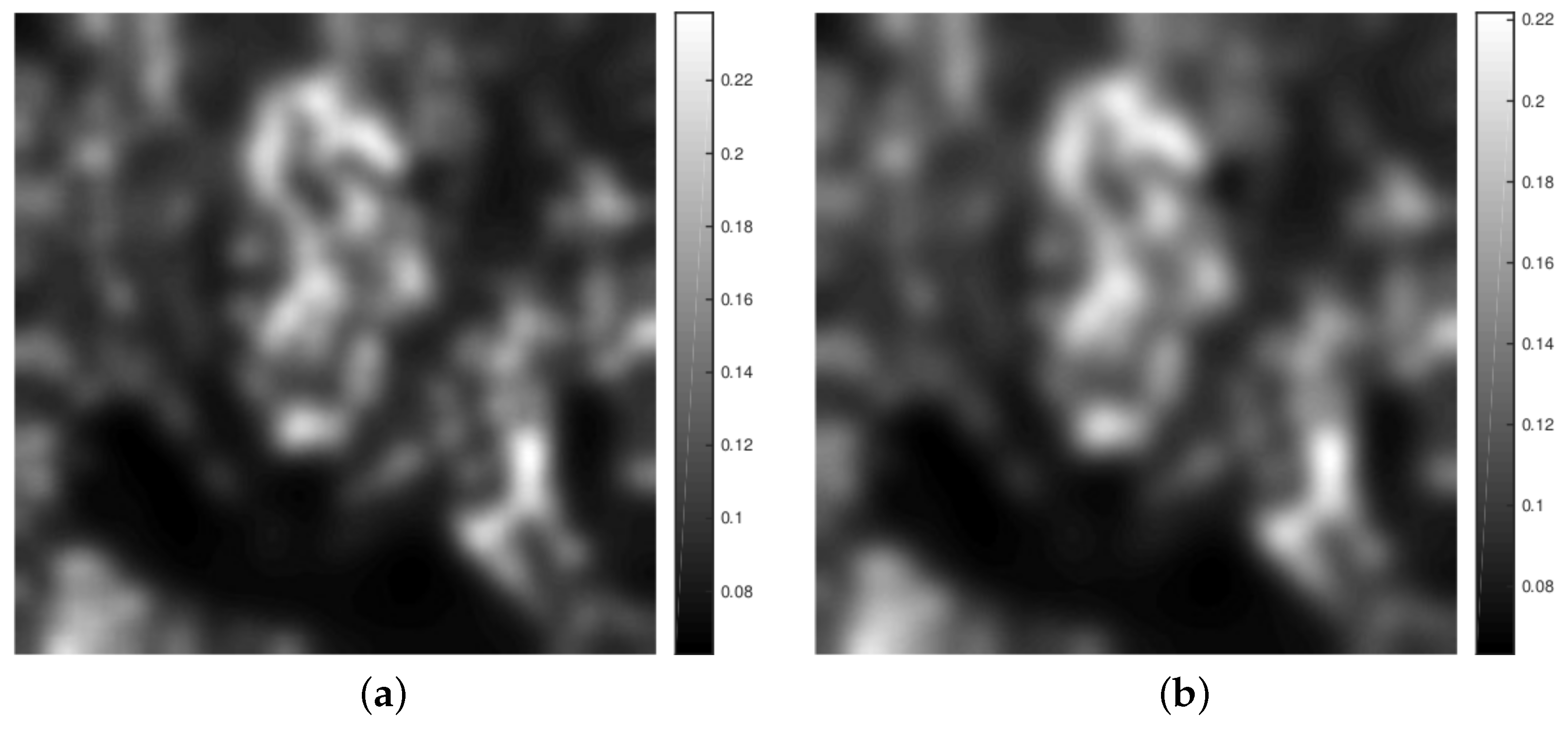
Figure 7.
Regularization parameter versus noise-level for the box-constrained pAPS in image deblurring.
Figure 7.
Regularization parameter versus noise-level for the box-constrained pAPS in image deblurring.
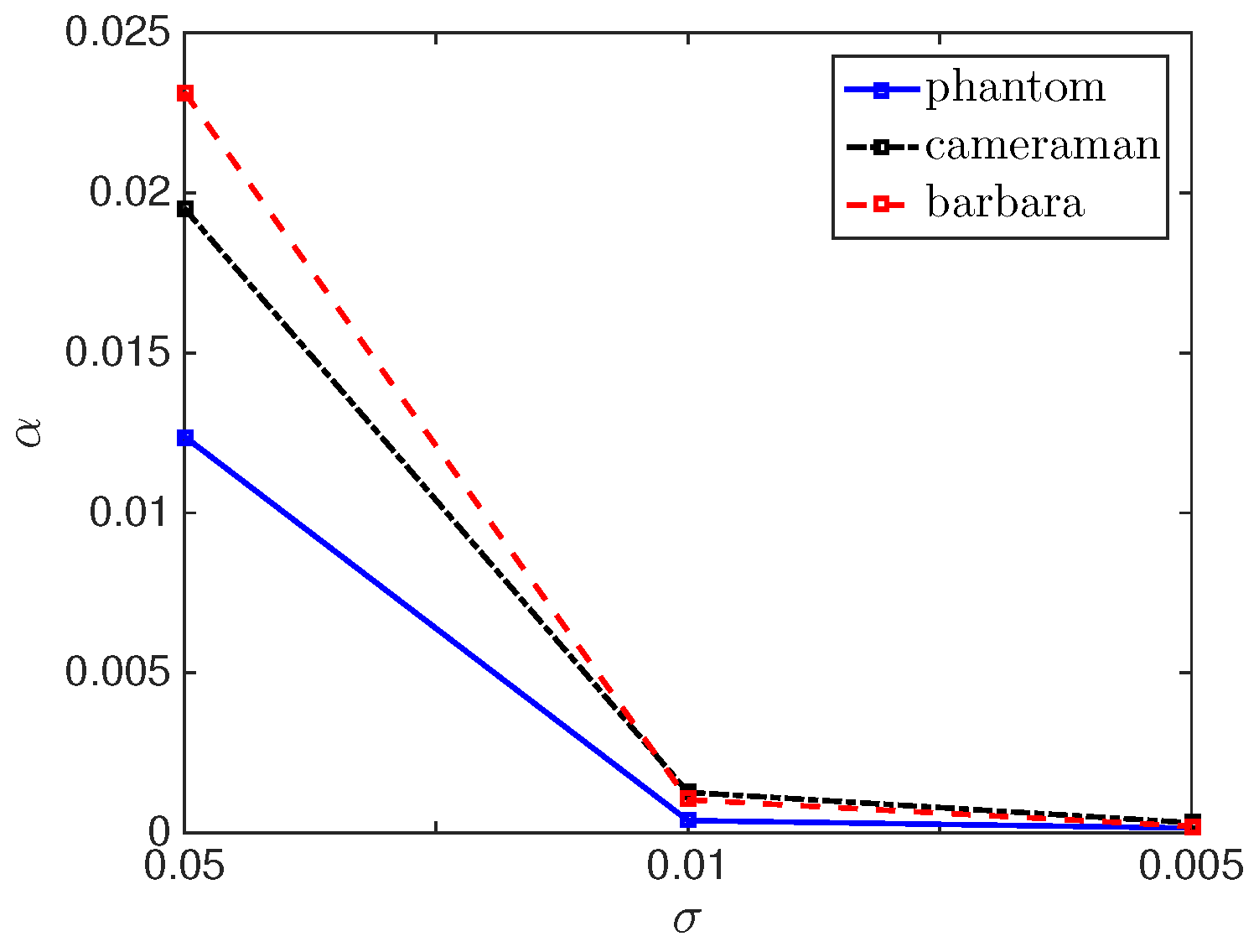
Figure 8.
Reconstruction from blurry and noisy data. (a) Blurry and noisy observation; (b) pAPS with pdN with (PSNR: 24.281; MSSIM: 0.34554); (c) pAPS with box-constrained pdN (PSNR: 24.293; MSSIM: 0.34618); (d) ADMM (PSNR: 24.236; MSSIM: 0.34073); (e) Box-constrained ADMM (PSNR: 24.237; MSSIM: 0.34082); (f) pLATV with pdN with (PSNR: 24.599; MSSIM: 0.34708); (g) pLATV with box-constrained pdN (PSNR: 24.622; MSSIM: 0.34769).

Figure 9.
Spatially varying regularization parameter generated by the respective pLATV-algorithm. (a) pLATV with pdN with ; (b) pLATV-algorithm with box-constrained pdN.
Figure 9.
Spatially varying regularization parameter generated by the respective pLATV-algorithm. (a) pLATV with pdN with ; (b) pLATV-algorithm with box-constrained pdN.
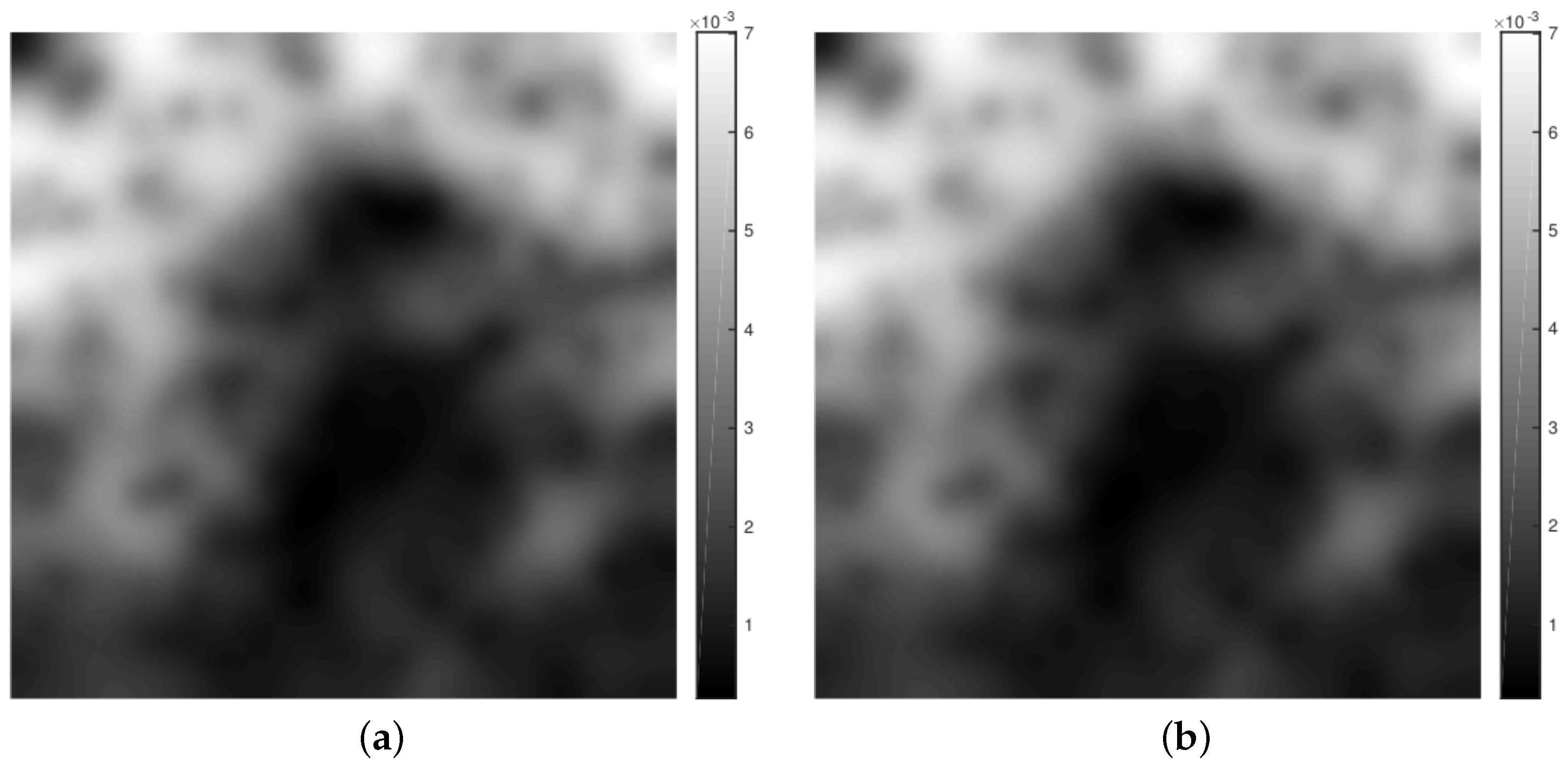
Figure 10.
Simultaneous image inpainting and denoising with . (a) Observation; (b) pAPS with pdN with (PSNR: 24.922; MSSIM: 0.44992); (c) pAPS with box-constrained pdN (PSNR: 24.922; MSSIM: 0.44992); (d) pLATV with pdN with (PSNR: 24.893; MSSIM: 0.4498); (e) pLATV with box-constrained pdN (PSNR: 24.868; MSSIM: 0.45004).

Figure 11.
Spatially varying regularization parameter generated by the respective pLATV-algorithm. (a) pLATV with pdN with ; (b) pLATV-algorithm with box-constrained pdN.
Figure 11.
Spatially varying regularization parameter generated by the respective pLATV-algorithm. (a) pLATV with pdN with ; (b) pLATV-algorithm with box-constrained pdN.

Figure 12.
Sampling domain in the frequency plane, i.e., sampling operator S.

Figure 13.
Reconstruction from sampled Fourier data. (a) pAPS with pdN with (PSNR: 25.017; MSSIM: 0.37061); (b) pAPS with box-constrained pdN (PSNR: 25.017; MSSIM: 0.37056); (c) pLATV with box-constrained pdN (PSNR: 23.64; MSSIM: 0.34945); (d) pLATV with pdN with (PSNR: 23.525; MSSIM: 0.34652).
Figure 13.
Reconstruction from sampled Fourier data. (a) pAPS with pdN with (PSNR: 25.017; MSSIM: 0.37061); (b) pAPS with box-constrained pdN (PSNR: 25.017; MSSIM: 0.37056); (c) pLATV with box-constrained pdN (PSNR: 23.64; MSSIM: 0.34945); (d) pLATV with pdN with (PSNR: 23.525; MSSIM: 0.34652).

Figure 14.
The Shepp-Logan phantom image of size pixels and its measured sinogram. (a) Original image; (b) Sinogram.
Figure 14.
The Shepp-Logan phantom image of size pixels and its measured sinogram. (a) Original image; (b) Sinogram.
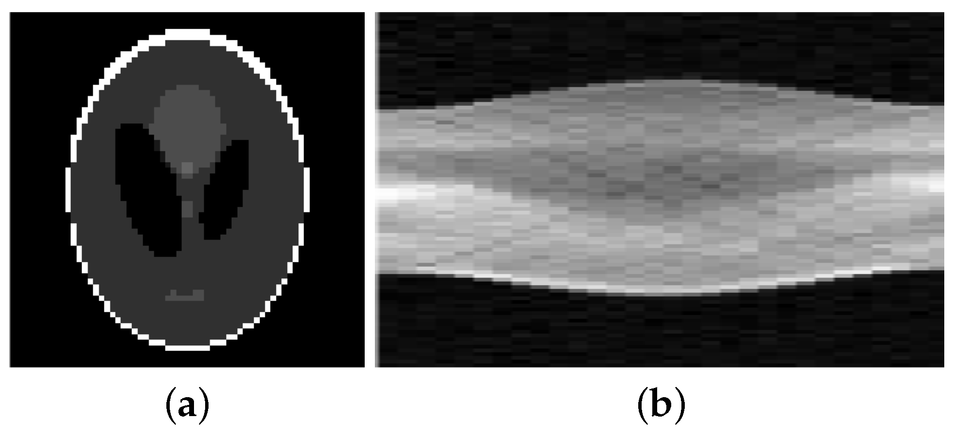
Figure 15.
Slice of a human head and its measured sinogram. (a) Original image; (b) Sinogram.

Figure 16.
Reconstruction from noisy data. (a) Inverse Radon-transform (PSNR: 29.08; MSSIM: 0.3906); (b) -TV (PSNR: 29.14; MSSIM: 0.4051); (c) Box-constrained -TV (PSNR: 33.31; MSSIM: 0.6128); (d) Inverse Radon-transform (PSNR: 31.75; MSSIM: 0.3699); (e) -TV (PSNR: 32.16; MSSIM: 0.3682); (f) Box-constrained -TV (PSNR: 36.08; MSSIM: 0.5856).


Table 1.
Reconstruction of the cameraman-image corrupted by Gaussian white noise with for different regularization parameters .
Table 1.
Reconstruction of the cameraman-image corrupted by Gaussian white noise with for different regularization parameters .
| pdN with | Box-Constrained pdN | |||||||
|---|---|---|---|---|---|---|---|---|
| PSNR | MSSIM | Time | It | PSNR | MSSIM | Time | It | |
| 0.001 | 20.165 | 0.27649 | 183.29 | 365 | 20.635 | 0.28384 | 178.27 | 365 |
| 0.01 | 21.464 | 0.29712 | 55.598 | 117 | 21.905 | 0.30472 | 55.245 | 117 |
| 0.096029 | 27.134 | 0.35214 | 14.615 | 33 | 27.135 | 0.35221 | 14.465 | 33 |
| 0.096108 | 27.132 | 0.35201 | 14.91 | 33 | 27.133 | 0.35207 | 14.317 | 33 |
| 0.4 | 22.079 | 0.16816 | 14.779 | 34 | 22.079 | 0.16816 | 14.982 | 34 |
| ⌀ | 23.5947 | 0.28919 | 56.6388 | 116.4 | 23.7773 | 0.2922 | 55.4557 | 116.4 |
Table 2.
Reconstruction of the cameraman-image corrupted by Gaussian blur and Gaussian white noise with for different regularization parameters .
Table 2.
Reconstruction of the cameraman-image corrupted by Gaussian blur and Gaussian white noise with for different regularization parameters .
| pdN with | Box-Constrained pdN | |||||||
|---|---|---|---|---|---|---|---|---|
| PSNR | MSSIM | Time | It | PSNR | MSSIM | Time | It | |
| 0.001 | 5.9375 | 0.039866 | 1197 | 143 | 11.568 | 0.083341 | 1946 | 145 |
| 0.01 | 21.908 | 0.18938 | 863 | 67 | 21.964 | 0.1946 | 2011 | 67 |
| 0.051871 | 21.815 | 0.18115 | 759 | 37 | 21.814 | 0.18113 | 1299 | 37 |
| 0.051868 | 21.814 | 0.18114 | 752 | 36 | 21.814 | 0.18114 | 1255 | 37 |
| 0.4 | 19.823 | 0.090709 | 1431 | 61 | 19.823 | 0.090709 | 1454 | 61 |
| ⌀ | 18.2593 | 0.13645 | 1000 | 68.8 | 19.3966 | 0.14618 | 1593 | 69.4 |
Table 3.
Reconstruction of the cameraman-image corrupted by Gaussian white noise with for different regularization parameters using the pdN with thresholded g.
Table 3.
Reconstruction of the cameraman-image corrupted by Gaussian white noise with for different regularization parameters using the pdN with thresholded g.
| PSNR | MSSIM | Time | It | |
|---|---|---|---|---|
| 0.001 | 20.64 | 0.28388 | 107.05 | 349 |
| 0.01 | 21.949 | 0.30504 | 32.336 | 113 |
| 0.096029 | 26.528 | 0.33078 | 8.9479 | 33 |
| 0.096108 | 26.526 | 0.33066 | 8.8966 | 33 |
| 0.4 | 21.666 | 0.15794 | 9.4218 | 35 |
| ⌀ | 23.4617 | 0.28166 | 33.3304 | 112.6 |
Table 4.
Reconstruction of the cameraman-image corrupted by Gaussian blur and Gaussian white noise with for different regularization parameters using the pdN with thresholded g.
Table 4.
Reconstruction of the cameraman-image corrupted by Gaussian blur and Gaussian white noise with for different regularization parameters using the pdN with thresholded g.
| PSNR | MSSIM | Time | It | |
|---|---|---|---|---|
| 0.001 | 6.6758 | 0.046454 | 1091 | 140 |
| 0.01 | 21.929 | 0.19231 | 743 | 65 |
| 0.051871 | 21.709 | 0.1722 | 659 | 35 |
| 0.051868 | 21.709 | 0.1722 | 651 | 35 |
| 0.4 | 19.683 | 0.087447 | 1438 | 61 |
| ⌀ | 18.3413 | 0.13412 | 916 | 67.2 |
Table 5.
Reconstruction of the cameraman-image corrupted by Gaussian white noise with standard deviation .
Table 5.
Reconstruction of the cameraman-image corrupted by Gaussian white noise with standard deviation .
| Box-Constrained pdN | Box-Constrained ADMM | ||||||||
|---|---|---|---|---|---|---|---|---|---|
| PSNR | MSSIM | Time | It | PSNR | MSSIM | Time | It | ||
| 0.3 | 0.34586 | 22.485 | 0.18619 | 18.844 | 41 | 22.2 | 0.17829 | 897.82 | 127 |
| 0.2 | 0.21408 | 24.054 | 0.24497 | 14.847 | 33 | 23.852 | 0.23917 | 808.67 | 100 |
| 0.1 | 0.096108 | 27.132 | 0.35201 | 14.91 | 33 | 26.963 | 0.35118 | 716.37 | 70 |
| 0.05 | 0.043393 | 30.567 | 0.47437 | 22.902 | 51 | 30.488 | 0.47503 | 656.66 | 48 |
| 0.01 | 0.0071847 | 40.417 | 0.75235 | 59.533 | 133 | 40.542 | 0.75864 | 454.45 | 24 |
| 0.005 | 0.0032996 | 45.164 | 0.8686 | 89.674 | 199 | 45.423 | 0.87718 | 501.59 | 24 |
| ⌀ | 31.6363 | 0.47975 | 36.785 | 81.667 | 31.5781 | 0.47991 | 672.5961 | 65.5 | |
Table 6.
Reconstruction of the cameraman-image corrupted by Gaussian blur and Gaussian white noise with standard deviation .
Table 6.
Reconstruction of the cameraman-image corrupted by Gaussian blur and Gaussian white noise with standard deviation .
| Box-Constrained pdN | Box-Constrained ADMM | ||||||||
|---|---|---|---|---|---|---|---|---|---|
| PSNR | MSSIM | Time | It | PSNR | MSSIM | Time | It | ||
| 0.3 | 0.2342 | 20.382 | 0.10678 | 1551.5 | 55 | 20.361 | 0.099691 | 2217.3 | 256 |
| 0.2 | 0.13169 | 20.981 | 0.13262 | 1434 | 41 | 20.978 | 0.12702 | 2593.1 | 265 |
| 0.1 | 0.051871 | 21.814 | 0.18113 | 1407.4 | 37 | 21.825 | 0.17536 | 3404.5 | 292 |
| 0.05 | 0.01951 | 22.484 | 0.22905 | 2691.4 | 51 | 22.501 | 0.22423 | 4065.4 | 305 |
| 0.01 | 0.0012674 | 24.293 | 0.34618 | 2440.5 | 126 | 24.237 | 0.34082 | 7185.3 | 358 |
| 0.005 | 0.00031869 | 25.451 | 0.40405 | 1903.4 | 149 | 25.377 | 0.3987 | 26,985 | 1081 |
| ⌀ | 22.5674 | 0.2333 | 1904.6943 | 76.5 | 22.5464 | 0.22764 | 7741.7188 | 426.17 | |
Table 7.
PSNR- and MSSIM-values of the reconstruction of different images corrupted by Gaussian white noise via pAPS using the primal-dual Newton method.
Table 7.
PSNR- and MSSIM-values of the reconstruction of different images corrupted by Gaussian white noise via pAPS using the primal-dual Newton method.
| Image | pAPS with pdN with | pAPS with Box-Constrained pdN | |||||||||
|---|---|---|---|---|---|---|---|---|---|---|---|
| PSNR | MSSIM | Time | It | PSNR | MSSIM | Time | It | ||||
| phantom | 0.3 | 19.274 | 0.30365 | 693.59 | 0.28721 | 40 | 19.302 | 0.30456 | 486.9 | 0.28544 | 20 |
| 0.2 | 22.024 | 0.37461 | 553.44 | 0.19055 | 37 | 22.06 | 0.37521 | 393.67 | 0.18921 | 17 | |
| 0.1 | 27.471 | 0.44124 | 565.80 | 0.09621 | 37 | 27.518 | 0.4412 | 389.39 | 0.095365 | 17 | |
| 0.05 | 33.173 | 0.46878 | 858.33 | 0.048744 | 37 | 33.228 | 0.46847 | 421.18 | 0.04827 | 16 | |
| 0.01 | 46.409 | 0.50613 | 1605.4 | 0.010597 | 37 | 46.46 | 0.50559 | 791.34 | 0.010509 | 17 | |
| 0.005 | 51.805 | 0.52587 | 2245.3 | 0.0057362 | 35 | 51.846 | 0.52522 | 925.46 | 0.0056958 | 15 | |
| cameraman | 0.3 | 22.485 | 0.18619 | 1591 | 0.34586 | 102 | 22.485 | 0.18621 | 847.53 | 0.34579 | 50 |
| 0.2 | 24.054 | 0.24497 | 919.63 | 0.21408 | 66 | 24.056 | 0.24508 | 528.85 | 0.21398 | 32 | |
| 0.1 | 27.132 | 0.35201 | 580.91 | 0.096108 | 39 | 27.135 | 0.35221 | 646.44 | 0.096029 | 41 | |
| 0.05 | 30.567 | 0.47437 | 549.23 | 0.043393 | 24 | 30.571 | 0.47458 | 561.43 | 0.04336 | 25 | |
| 0.01 | 40.417 | 0.75235 | 677.79 | 0.0071847 | 12 | 40.418 | 0.75238 | 645.32 | 0.0071837 | 12 | |
| 0.005 | 45.164 | 0.8686 | 745.67 | 0.0032996 | 9 | 45.164 | 0.8686 | 701.1 | 0.0032995 | 9 | |
| barbara | 0.3 | 20.618 | 0.30666 | 1419.7 | 0.34118 | 84 | 20.618 | 0.30666 | 735.83 | 0.34118 | 39 |
| 0.2 | 21.649 | 0.39964 | 788.49 | 0.20109 | 47 | 21.649 | 0.39971 | 358.6 | 0.20105 | 18 | |
| 0.1 | 24.241 | 0.58555 | 336.17 | 0.089758 | 23 | 24.241 | 0.58564 | 319.09 | 0.089746 | 23 | |
| 0.05 | 27.884 | 0.75178 | 326.59 | 0.04286 | 15 | 27.885 | 0.7518 | 286.61 | 0.042858 | 16 | |
| 0.01 | 38.781 | 0.9322 | 345.64 | 0.0079133 | 9 | 38.781 | 0.9322 | 311.25 | 0.0079133 | 9 | |
| 0.005 | 44.056 | 0.9681 | 395.8 | 0.0037205 | 7 | 44.056 | 0.9681 | 330.97 | 0.0037205 | 7 | |
| house | 0.3 | 23.827 | 0.1839 | 2750 | 0.41771 | 154 | 23.829 | 0.18392 | 1185.9 | 0.41763 | 75 |
| 0.2 | 25.611 | 0.23397 | 1460.6 | 0.26795 | 116 | 25.611 | 0.23397 | 610.2 | 0.26796 | 45 | |
| 0.1 | 28.855 | 0.31916 | 690.33 | 0.11979 | 75 | 28.855 | 0.31916 | 348.92 | 0.11979 | 34 | |
| 0.05 | 32.04 | 0.4074 | 574.34 | 0.050505 | 39 | 32.041 | 0.40741 | 563.92 | 0.050502 | 40 | |
| 0.01 | 40.292 | 0.75174 | 493.84 | 0.0071206 | 11 | 40.292 | 0.75174 | 468.11 | 0.0071206 | 11 | |
| 0.005 | 44.989 | 0.86648 | 527 | 0.0033035 | 8 | 44.989 | 0.86648 | 502.38 | 0.0033035 | 8 | |
| lena | 0.3 | 21.905 | 0.29155 | 1925 | 0.41731 | 120 | 21.905 | 0.29155 | 953.83 | 0.41731 | 57 |
| 0.2 | 23.506 | 0.36317 | 1064.9 | 0.25937 | 85 | 23.506 | 0.36317 | 585.24 | 0.25937 | 39 | |
| 0.1 | 26.37 | 0.49351 | 537.69 | 0.11246 | 46 | 26.369 | 0.49351 | 302.32 | 0.11246 | 21 | |
| 0.05 | 29.615 | 0.62313 | 566.71 | 0.047771 | 27 | 29.615 | 0.62313 | 579.3 | 0.04777 | 28 | |
| 0.01 | 39.261 | 0.91371 | 526.89 | 0.0068096 | 97 | 39.262 | 0.91371 | 546.75 | 0.0068091 | 10 | |
| 0.005 | 44.672 | 0.97133 | 626.47 | 0.0032764 | 8 | 44.673 | 0.97133 | 652.97 | 0.0032762 | 8 | |
| bones | 0.3 | 25.744 | 0.34395 | 5830.2 | 0.86048 | 310 | 25.743 | 0.34395 | 749.26 | 0.8605 | 35 |
| 0.2 | 27.637 | 0.39821 | 2949 | 0.56086 | 238 | 27.637 | 0.39821 | 747.28 | 0.56086 | 45 | |
| 0.1 | 30.908 | 0.49398 | 1232.8 | 0.27216 | 141 | 30.908 | 0.49398 | 364.71 | 0.27216 | 32 | |
| 0.05 | 34.284 | 0.58386 | 612.74 | 0.12735 | 87 | 34.284 | 0.58386 | 362.62 | 0.12735 | 41 | |
| 0.01 | 43.174 | 0.7449 | 386.03 | 0.020815 | 33 | 43.174 | 0.7449 | 479.77 | 0.020814 | 33 | |
| 0.005 | 47.493 | 0.80124 | 340.02 | 0.0091423 | 23 | 47.493 | 0.80124 | 470.83 | 0.0091423 | 23 | |
| cookies | 0.3 | 21.466 | 0.31394 | 1117.4 | 0.38254 | 87 | 21.466 | 0.31396 | 857.99 | 0.38252 | 42 |
| 0.2 | 23.136 | 0.40787 | 709.8 | 0.25117 | 62 | 23.136 | 0.40787 | 320.84 | 0.25118 | 12 | |
| 0.1 | 26.498 | 0.55614 | 398.59 | 0.12598 | 42 | 26.498 | 0.55614 | 290.67 | 0.12598 | 18 | |
| 0.05 | 30.292 | 0.67741 | 382.29 | 0.06257 | 30 | 30.293 | 0.67741 | 523.47 | 0.06257 | 30 | |
| 0.01 | 40.482 | 0.85926 | 414.09 | 0.011324 | 15 | 40.482 | 0.85926 | 567.65 | 0.011324 | 15 | |
| 0.005 | 45.39 | 0.91128 | 470.54 | 0.0052653 | 12 | 45.39 | 0.91128 | 653.55 | 0.0052653 | 12 | |
| numbers | 0.3 | 17.593 | 0.33171 | 520.53 | 0.27654 | 31 | 17.862 | 0.35167 | 358.5 | 0.26337 | 6 |
| 0.2 | 20.658 | 0.39035 | 415.03 | 0.18442 | 30 | 20.936 | 0.40758 | 375.14 | 0.17526 | 9 | |
| 0.1 | 26.259 | 0.44549 | 365.01 | 0.092576 | 30 | 26.56 | 0.45925 | 318.58 | 0.087618 | 8 | |
| 0.05 | 32.061 | 0.47618 | 466.24 | 0.046674 | 30 | 32.382 | 0.48698 | 321.63 | 0.044044 | 8 | |
| 0.01 | 45.511 | 0.51733 | 1039 | 0.0099524 | 31 | 45.869 | 0.52176 | 467.07 | 0.0093273 | 7 | |
| 0.005 | 51.036 | 0.53022 | 1474.9 | 0.0053171 | 30 | 51.44 | 0.53149 | 463.78 | 0.0049401 | 5 | |
| ⌀ | 32.0368 | 0.5343 | 9,597,189 | 54.5833 | 32.0828 | 0.5357 | 534.877 | 23.75 | |||
Table 8.
PSNR- and MSSIM-values of the reconstruction of different images corrupted by Gaussian white noise via the ADMM by solving the constrained versions.
Table 8.
PSNR- and MSSIM-values of the reconstruction of different images corrupted by Gaussian white noise via the ADMM by solving the constrained versions.
| Image | ADMM | Box-Constrained ADMM | |||||||
|---|---|---|---|---|---|---|---|---|---|
| PSNR | MSSIM | Time | It | PSNR | MSSIM | Time | It | ||
| phantom | 0.3 | 18.956 | 0.29789 | 1245 | 118 | 18.922 | 0.29225 | 999.39 | 137 |
| 0.2 | 21.615 | 0.37299 | 1203.8 | 108 | 21.538 | 0.36632 | 1068.9 | 123 | |
| 0.1 | 27.021 | 0.45439 | 868.12 | 79 | 26.941 | 0.44525 | 995.99 | 91 | |
| 0.05 | 32.823 | 0.5007 | 576.35 | 47 | 32.731 | 0.4847 | 650.9 | 53 | |
| 0.01 | 46.446 | 0.60023 | 444.34 | 23 | 47.36 | 0.54521 | 524.88 | 27 | |
| 0.005 | 53.734 | 0.5907 | 566.53 | 24 | 53.59 | 0.51937 | 913.28 | 38 | |
| cameraman | 0.3 | 22.33 | 0.18003 | 889.65 | 99 | 22.2 | 0.17829 | 897.82 | 127 |
| 0.2 | 23.895 | 0.23961 | 836.26 | 80 | 23.852 | 0.23917 | 808.67 | 100 | |
| 0.1 | 27.002 | 0.35006 | 690.45 | 60 | 26.963 | 0.35118 | 716.37 | 70 | |
| 0.05 | 30.513 | 0.47359 | 564.73 | 43 | 30.488 | 0.47503 | 656.66 | 48 | |
| 0.01 | 40.486 | 0.75493 | 409.62 | 22 | 40.542 | 0.75864 | 454.45 | 24 | |
| 0.005 | 45.329 | 0.8728 | 494.94 | 23 | 45.423 | 0.87718 | 501.59 | 24 | |
| barbara | 0.3 | 20.6 | 0.30878 | 891.68 | 94 | 20.604 | 0.31256 | 683.92 | 112 |
| 0.2 | 21.655 | 0.40225 | 827.72 | 74 | 21.654 | 0.40468 | 628.45 | 91 | |
| 0.1 | 24.224 | 0.5883 | 583.96 | 50 | 24.215 | 0.58921 | 547.54 | 61 | |
| 0.05 | 27.889 | 0.75319 | 449.51 | 35 | 27.874 | 0.75405 | 470.8 | 41 | |
| 0.01 | 38.921 | 0.9338 | 441.87 | 21 | 38.978 | 0.9341 | 374.69 | 24 | |
| 0.005 | 44.413 | 0.97035 | 503.68 | 21 | 44.584 | 0.97166 | 425.92 | 23 | |
| house | 0.3 | 23.761 | 0.19254 | 1072.7 | 108 | 23.689 | 0.19468 | 674.76 | 128 |
| 0.2 | 25.659 | 0.24287 | 949.97 | 85 | 25.609 | 0.24367 | 709.26 | 108 | |
| 0.1 | 28.907 | 0.32034 | 678 | 54 | 28.875 | 0.32115 | 596.95 | 70 | |
| 0.05 | 32.054 | 0.40609 | 532.99 | 35 | 32.029 | 0.40732 | 478.67 | 42 | |
| 0.01 | 40.394 | 0.7555 | 422.07 | 19 | 40.438 | 0.75891 | 331.36 | 21 | |
| 0.005 | 45.201 | 0.87241 | 492.11 | 20 | 45.278 | 0.8758 | 408.17 | 22 | |
| lena | 0.3 | 21.834 | 0.29247 | 950.81 | 102 | 21.85 | 0.2995 | 570.59 | 115 |
| 0.2 | 23.455 | 0.36437 | 724 | 81 | 23.46 | 0.36828 | 670.96 | 97 | |
| 0.1 | 26.349 | 0.49495 | 584.08 | 55 | 26.333 | 0.49605 | 641.47 | 67 | |
| 0.05 | 29.604 | 0.62425 | 456.63 | 39 | 29.588 | 0.62541 | 554.51 | 44 | |
| 0.01 | 39.422 | 0.91694 | 377.76 | 22 | 39.486 | 0.91822 | 438.7 | 25 | |
| 0.005 | 45.021 | 0.97391 | 470.81 | 24 | 45.106 | 0.97436 | 517.97 | 26 | |
| bones | 0.3 | 25.829 | 0.35686 | 750.12 | 110 | 25.051 | 0.36748 | 611.23 | 115 |
| 0.2 | 27.689 | 0.40363 | 734.13 | 90 | 27.486 | 0.41281 | 652.2 | 94 | |
| 0.1 | 30.942 | 0.48823 | 624.02 | 58 | 31.02 | 0.49267 | 755.06 | 75 | |
| 0.05 | 34.319 | 0.57951 | 343.83 | 35 | 34.37 | 0.57521 | 624.7 | 49 | |
| 0.01 | 43.011 | 0.73032 | 193.87 | 14 | 42.9 | 0.72002 | 270.92 | 16 | |
| 0.005 | 47.446 | 0.79549 | 204.98 | 12 | 47.432 | 0.78519 | 285.72 | 14 | |
| cookies | 0.3 | 21.436 | 0.31503 | 789.78 | 102 | 21.461 | 0.32264 | 788.24 | 118 |
| 0.2 | 23.129 | 0.40742 | 713.25 | 82 | 23.128 | 0.41261 | 772.93 | 99 | |
| 0.1 | 26.527 | 0.55478 | 554.95 | 55 | 26.506 | 0.55871 | 659.5 | 70 | |
| 0.05 | 30.364 | 0.67447 | 422.84 | 37 | 30.338 | 0.67746 | 589.77 | 45 | |
| 0.01 | 40.513 | 0.85593 | 234.35 | 15 | 40.589 | 0.85815 | 316.64 | 19 | |
| 0.005 | 45.382 | 0.90918 | 255.79 | 14 | 45.307 | 0.90892 | 319.82 | 16 | |
| numbers | 0.3 | 17.257 | 0.32157 | 1640.7 | 147 | 17.487 | 0.34599 | 1311.9 | 146 |
| 0.2 | 20.279 | 0.38382 | 1594 | 133 | 20.49 | 0.42 | 1215.8 | 134 | |
| 0.1 | 25.901 | 0.44284 | 981.06 | 95 | 26.125 | 0.48656 | 874.87 | 85 | |
| 0.05 | 31.847 | 0.47604 | 719.72 | 52 | 32.412 | 0.51241 | 532.91 | 46 | |
| 0.01 | 45.726 | 0.52365 | 643.88 | 26 | 47.089 | 0.51102 | 1001.3 | 56 | |
| 0.005 | 52.512 | 0.53468 | 641.43 | 29 | 52.859 | 0.51942 | 1756.9 | 83 | |
| ⌀ | 32.0754 | 0.5386 | 671.7274 | 57.7292 | 32.1302 | 0.5389 | 671.9570 | 67.8958 | |
Table 9.
PSNR- and MSSIM-values of the reconstruction of different images corrupted by Gaussian white noise via pLATV using the primal-dual Newton method.
Table 9.
PSNR- and MSSIM-values of the reconstruction of different images corrupted by Gaussian white noise via pLATV using the primal-dual Newton method.
| Image | pLATV with pdN with | pLATV with Box-Constrained pdN | |||||||
|---|---|---|---|---|---|---|---|---|---|
| PSNR | MSSIM | Time | It | PSNR | MSSIM | Time | It | ||
| phantom | 0.3 | 19.629 | 0.31986 | 517.78 | 13 | 19.744 | 0.32143 | 710.59 | 16 |
| 0.2 | 22.405 | 0.38578 | 286.66 | 13 | 22.525 | 0.38706 | 607.27 | 15 | |
| 0.1 | 27.802 | 0.44701 | 389.34 | 13 | 27.936 | 0.44762 | 552.49 | 14 | |
| 0.05 | 33.48 | 0.47301 | 526.89 | 13 | 33.57 | 0.4733 | 571.06 | 14 | |
| 0.01 | 46.546 | 0.50749 | 139.72 | 4 | 46.625 | 0.50646 | 98.973 | 3 | |
| 0.005 | 52.038 | 0.52569 | 112.1 | 3 | 52.062 | 0.52512 | 105.89 | 3 | |
| cameraman | 0.3 | 22.382 | 0.18185 | 775.5 | 15 | 22.393 | 0.18186 | 838.55 | 19 |
| 0.2 | 24.032 | 0.24038 | 605.56 | 13 | 24.029 | 0.23937 | 593.9 | 16 | |
| 0.1 | 27.16 | 0.35301 | 304.83 | 12 | 27.175 | 0.35285 | 415.09 | 13 | |
| 0.05 | 30.702 | 0.4745 | 310.03 | 10 | 30.696 | 0.47315 | 262.59 | 10 | |
| 0.01 | 40.647 | 0.73386 | 135.88 | 4 | 40.647 | 0.73386 | 144.01 | 4 | |
| 0.005 | 45.292 | 0.86678 | 365.19 | 7 | 45.292 | 0.86678 | 357.42 | 7 | |
| barbara | 0.3 | 20.527 | 0.30278 | 572.44 | 16 | 20.516 | 0.3023 | 652.83 | 18 |
| 0.2 | 21.73 | 0.39872 | 411.5 | 13 | 21.729 | 0.39882 | 459.09 | 14 | |
| 0.1 | 24.503 | 0.58885 | 285.8 | 9 | 24.486 | 0.58693 | 302.46 | 10 | |
| 0.05 | 28.196 | 0.75135 | 309.53 | 7 | 28.198 | 0.75151 | 304.89 | 7 | |
| 0.01 | 38.898 | 0.92794 | 424.8 | 18 | 38.898 | 0.92794 | 425.12 | 18 | |
| 0.005 | 44.186 | 0.96871 | 147.57 | 5 | 44.186 | 0.96871 | 150.91 | 5 | |
| house | 0.3 | 23.661 | 0.18529 | 593.22 | 18 | 23.704 | 0.18526 | 698.35 | 22 |
| 0.2 | 25.507 | 0.23789 | 478.33 | 17 | 25.51 | 0.23741 | 522.86 | 18 | |
| 0.1 | 28.736 | 0.32695 | 304.43 | 13 | 28.741 | 0.32581 | 332.47 | 14 | |
| 0.05 | 31.94 | 0.4217 | 184.75 | 11 | 31.943 | 0.42182 | 320.22 | 11 | |
| 0.01 | 40.423 | 0.73752 | 451.47 | 13 | 40.423 | 0.73752 | 377.89 | 13 | |
| 0.005 | 45.118 | 0.85458 | 286.48 | 7 | 45.118 | 0.85458 | 222.54 | 7 | |
| lena | 0.3 | 21.829 | 0.29245 | 624.96 | 19 | 21.828 | 0.29232 | 727.69 | 21 |
| 0.2 | 23.442 | 0.3634 | 471.91 | 16 | 23.445 | 0.36326 | 538.81 | 17 | |
| 0.1 | 26.403 | 0.49438 | 347.04 | 13 | 26.406 | 0.49419 | 374.1 | 14 | |
| 0.05 | 29.703 | 0.62778 | 396.43 | 8 | 29.704 | 0.62784 | 403.49 | 8 | |
| 0.01 | 39.324 | 0.91256 | 652.2 | 16 | 39.324 | 0.91256 | 659.92 | 16 | |
| 0.005 | 44.736 | 0.97081 | 244.61 | 5 | 44.737 | 0.97081 | 237.28 | 5 | |
| bones | 0.3 | 25.633 | 0.36194 | 869.22 | 37 | 25.518 | 0.35855 | 1122.8 | 38 |
| 0.2 | 27.6 | 0.41895 | 665.85 | 33 | 27.506 | 0.41674 | 823.95 | 33 | |
| 0.1 | 30.964 | 0.51162 | 419.72 | 26 | 30.862 | 0.51085 | 435.6 | 24 | |
| 0.05 | 34.413 | 0.59991 | 291.13 | 19 | 34.408 | 0.59947 | 374.07 | 19 | |
| 0.01 | 43.521 | 0.76261 | 98.45 | 6 | 43.521 | 0.76261 | 93.765 | 6 | |
| 0.005 | 47.564 | 0.7997 | 103.29 | 6 | 47.564 | 0.7997 | 95.637 | 6 | |
| cookies | 0.3 | 21.415 | 0.31722 | 597.85 | 17 | 21.371 | 0.3164 | 653.83 | 18 |
| 0.2 | 23.126 | 0.40895 | 500.29 | 16 | 23.107 | 0.4087 | 485.2 | 15 | |
| 0.1 | 26.487 | 0.55758 | 237.87 | 12 | 26.501 | 0.55811 | 332.12 | 12 | |
| 0.05 | 30.301 | 0.68332 | 413.36 | 12 | 30.295 | 0.68292 | 175.11 | 9 | |
| 0.01 | 40.525 | 0.86052 | 261.76 | 8 | 40.525 | 0.86052 | 236.96 | 8 | |
| 0.005 | 45.499 | 0.90364 | 229.85 | 5 | 45.499 | 0.90364 | 174.58 | 5 | |
| numbers | 0.3 | 17.627 | 0.33232 | 421.86 | 11 | 17.821 | 0.34957 | 654.22 | 20 |
| 0.2 | 20.7 | 0.39072 | 313.32 | 10 | 20.888 | 0.40559 | 556.07 | 19 | |
| 0.1 | 26.296 | 0.4455 | 258.05 | 10 | 26.528 | 0.45766 | 440.13 | 17 | |
| 0.05 | 32.104 | 0.47624 | 339.03 | 10 | 32.369 | 0.48578 | 501.47 | 15 | |
| 0.01 | 45.527 | 0.51735 | 92.644 | 2 | 45.938 | 0.52169 | 59.513 | 2 | |
| 0.005 | 51.265 | 0.53078 | 207.86 | 5 | 51.536 | 0.53125 | 257.45 | 6 | |
| ⌀ | 32.1155 | 0.5365 | 374.5490 | 12.2708 | 32.1531 | 0.5375 | 425.8590 | 13.4167 | |
Table 10.
PSNR- and MSSIM-values of the reconstruction of different images corrupted by Gaussian blur and Gaussian white noise via pAPS or pLATV using the primal-dual Newton method or via the ADMM by solving the constrained versions.
Table 10.
PSNR- and MSSIM-values of the reconstruction of different images corrupted by Gaussian blur and Gaussian white noise via pAPS or pLATV using the primal-dual Newton method or via the ADMM by solving the constrained versions.
| Image | pAPS with pdN with | pAPS with Box-Constrained pdN | |||||||
| PSNR | MSSIM | Time | It | PSNR | MSSIM | Time | It | ||
| phantom | 0.05 | 16.41 | 0.21695 | 11,603 | 11 | 16.801 | 0.23085 | 33,002 | 11 |
| 0.01 | 18.624 | 0.30997 | 12,663 | 10 | 18.861 | 0.32574 | 18,744 | 8 | |
| 0.005 | 20.554 | 0.36713 | 5892.9 | 6 | 21.01 | 0.38225 | 17,245 | 9 | |
| cameraman | 0.05 | 22.482 | 0.2288 | 8328.5 | 11 | 22.484 | 0.22905 | 24,162 | 11 |
| 0.01 | 24.281 | 0.34554 | 4799.8 | 5 | 24.293 | 0.34618 | 13,102 | 5 | |
| 0.005 | 25.436 | 0.4035 | 5611.4 | 8 | 25.451 | 0.40405 | 12,033 | 7 | |
| barbara | 0.05 | 21.363 | 0.37833 | 5422.8 | 8 | 21.363 | 0.37832 | 10,657 | 8 |
| 0.01 | 22.052 | 0.49312 | 2820.6 | 5 | 22.052 | 0.49311 | 6188.1 | 5 | |
| 0.005 | 23.084 | 0.57223 | 4275.5 | 13 | 23.084 | 0.57223 | 11,121 | 13 | |
| ⌀ | 21.5874 | 0.3684 | 6824 | 8.5556 | 21.7108 | 0.37353 | 16,250 | 8.5556 | |
| Image | ADMM | Box-Constrained ADMM | |||||||
| PSNR | MSSIM | Time | It | PSNR | MSSIM | Time | It | ||
| phantom | 0.05 | 16.427 | 0.2691 | 6243.1 | 465 | 16.811 | 0.27613 | 8186.6 | 581 |
| 0.01 | 18.581 | 0.3094 | 34,683 | 1424 | 18.809 | 0.32544 | 33,141 | 1327 | |
| 0.005 | 20.505 | 0.3677 | 40,801 | 1426 | 20.906 | 0.38285 | 43,753 | 1485 | |
| cameraman | 0.05 | 22.51 | 0.2242 | 2870.1 | 214 | 22.501 | 0.22423 | 4065.4 | 305 |
| 0.01 | 24.236 | 0.34073 | 8268.2 | 428 | 24.237 | 0.34082 | 7185.3 | 358 | |
| 0.005 | 25.373 | 0.3986 | 30,944 | 1200 | 25.377 | 0.3987 | 26985 | 1081 | |
| barbara | 0.05 | 21.417 | 0.38039 | 1996.6 | 169 | 21.421 | 0.38113 | 2807.4 | 237 |
| 0.01 | 22.036 | 0.48965 | 13,282 | 678 | 22.038 | 0.48964 | 12,012 | 627 | |
| 0.005 | 23.043 | 0.56871 | 40,949 | 1527 | 23.038 | 0.56841 | 37,430 | 1423 | |
| ⌀ | 21.5699 | 0.37205 | 20,004 | 836.78 | 21.6821 | 0.37637 | 19,507 | 824.89 | |
| Image | pLATV with pdN with | pLATV with Box-Constrained pdN | |||||||
| PSNR | MSSIM | Time | It | PSNR | MSSIM | Time | It | ||
| phantom | 0.05 | 16.43 | 0.21966 | 14,732 | 12 | 16.824 | 0.23305 | 29,567 | 10 |
| 0.01 | 18.967 | 0.31788 | 39,014 | 49 | 19.602 | 0.33679 | 11,950 | 52 | |
| 0.005 | 20.729 | 0.36861 | 49,658 | 67 | 22.041 | 0.39052 | 11,940 | 71 | |
| cameraman | 0.05 | 22.533 | 0.22964 | 26,380 | 22 | 22.534 | 0.22973 | 70,208 | 22 |
| 0.01 | 24.599 | 0.34708 | 57,513 | 47 | 24.622 | 0.34769 | 113,175 | 47 | |
| 0.005 | 25.77 | 0.40389 | 39,662 | 60 | 25.796 | 0.40451 | 110,646 | 60 | |
| barbara | 0.05 | 21.377 | 0.3808 | 26,779 | 24 | 21.377 | 0.3808 | 49,808 | 24 |
| 0.01 | 22.432 | 0.50565 | 22,433 | 51 | 22.448 | 0.50625 | 78,720 | 52 | |
| 0.005 | 23.652 | 0.59532 | 16,168 | 61 | 23.658 | 0.59545 | 53,559 | 61 | |
| ⌀ | 21.8319 | 0.37428 | 32,482 | 43.667 | 22.1003 | 0.38053 | 81,893 | 44.333 | |
Table 11.
PSNR- and MSSIM-values for the application inpainting via pAPS.
| Image | pAPS with pdN with | pAPS with Box-Constrained pdN | |||||||||
|---|---|---|---|---|---|---|---|---|---|---|---|
| PSNR | MSSIM | Time | It | PSNR | MSSIM | Time | It | ||||
| lena | 0.3 | 21.151 | 0.26378 | 1709.9 | 0.37358 | 105 | 21.151 | 0.26378 | 958.59 | 0.37358 | 50 |
| 0.2 | 22.555 | 0.33033 | 1075.8 | 0.23336 | 72 | 22.555 | 0.33032 | 578.35 | 0.23336 | 32 | |
| 0.1 | 24.922 | 0.44992 | 578.34 | 0.10369 | 41 | 24.922 | 0.44992 | 370.42 | 0.10369 | 18 | |
| 0.05 | 27.005 | 0.56734 | 513.1 | 0.044922 | 25 | 27.005 | 0.56735 | 507.37 | 0.044919 | 25 | |
| 0.01 | 29.618 | 0.82318 | 524.73 | 0.006614 | 9 | 29.618 | 0.82319 | 516.86 | 0.0066133 | 9 | |
| 0.005 | 29.912 | 0.87427 | 569.85 | 0.00319 | 8 | 29.912 | 0.87427 | 674.02 | 0.0031896 | 8 | |
| cookies | 0.3 | 20.761 | 0.27956 | 1189.8 | 0.34456 | 74 | 20.763 | 0.27963 | 806.65 | 0.34448 | 35 |
| 0.2 | 22.138 | 0.36599 | 761.34 | 0.22529 | 55 | 22.138 | 0.36599 | 228.76 | 0.22529 | 10 | |
| 0.1 | 24.624 | 0.50595 | 419.34 | 0.11088 | 36 | 24.624 | 0.50595 | 283.69 | 0.11088 | 15 | |
| 0.05 | 26.967 | 0.62721 | 359.67 | 0.05467 | 26 | 26.967 | 0.62721 | 409.44 | 0.05467 | 26 | |
| 0.01 | 30.05 | 0.80847 | 481.89 | 0.01008 | 14 | 30.05 | 0.80847 | 547.4 | 0.01008 | 14 | |
| 0.005 | 30.438 | 0.85701 | 491.23 | 0.0047745 | 11 | 30.438 | 0.85701 | 590.77 | 0.0047745 | 11 | |
| ⌀ | 25.83 | 0.57403 | 617.22 | 36 | 25.83 | 0.57404 | 477.78 | 18.5 | |||
Table 12.
PSNR- and MSSIM-values for the application inpainting via pLATV.
| Image | pLATV with pdN with | pLATV with Box-Constrained pdN | |||||||
|---|---|---|---|---|---|---|---|---|---|
| PSNR | MSSIM | Time | It | PSNR | MSSIM | Time | It | ||
| lena | 0.3 | 21.027 | 0.26266 | 684.18 | 14 | 21.036 | 0.26239 | 836.18 | 16 |
| 0.2 | 22.45 | 0.32986 | 555.66 | 11 | 22.457 | 0.32939 | 584.66 | 12 | |
| 0.1 | 24.893 | 0.4498 | 446.84 | 12 | 24.868 | 0.45004 | 400.3 | 9 | |
| 0.05 | 26.982 | 0.56904 | 474.61 | 9 | 26.983 | 0.56912 | 460.22 | 9 | |
| 0.01 | 29.621 | 0.82242 | 796.53 | 16 | 29.621 | 0.82242 | 775.88 | 16 | |
| 0.005 | 29.987 | 0.87461 | 285.24 | 5 | 29.987 | 0.87461 | 284.79 | 5 | |
| cookies | 0.3 | 20.546 | 0.27499 | 660.05 | 11 | 20.548 | 0.27574 | 753.89 | 13 |
| 0.2 | 21.965 | 0.36179 | 458.1 | 10 | 21.975 | 0.36259 | 578.94 | 11 | |
| 0.1 | 24.538 | 0.50627 | 193.2 | 10 | 24.547 | 0.50651 | 251.68 | 11 | |
| 0.05 | 26.862 | 0.63007 | 322.75 | 7 | 26.863 | 0.6301 | 381.66 | 7 | |
| 0.01 | 30.047 | 0.80869 | 83.563 | 2 | 30.047 | 0.80869 | 99.415 | 2 | |
| 0.005 | 30.254 | 0.84914 | 181.44 | 5 | 30.254 | 0.84914 | 213.15 | 5 | |
| ⌀ | 25.7643 | 0.56161 | 428.51 | 9.3333 | 25.765 | 0.56173 | 468.3961 | 9.6667 | |
Table 13.
PSNR- and MSSIM-values of the reconstruction of sampled Fourier data corrupted by Gaussian white noise via the pAPS- and pLATV-algorithm using the primal-dual Newton method.
Table 13.
PSNR- and MSSIM-values of the reconstruction of sampled Fourier data corrupted by Gaussian white noise via the pAPS- and pLATV-algorithm using the primal-dual Newton method.
| Image | pAPS with pdN with | pAPS with Box-Constrained pdN | |||||
| PSNR | MSSIM | CPU-Time | PSNR | MSSIM | CPU-Time | ||
| Shepp- | 0.3 | 18.888 | 0.16233 | 3787.2 | 19.000 | 0.1685 | 5509.2 |
| Logan | 0.2 | 20.524 | 0.21302 | 2844.9 | 20.696 | 0.22086 | 3673.5 |
| phantom | 0.1 | 24.256 | 0.2905 | 1884.7 | 24.496 | 0.29896 | 2582.3 |
| 0.05 | 28.639 | 0.34972 | 2008.5 | 28.948 | 0.35833 | 2115 | |
| 0.01 | 40.168 | 0.42734 | 1993.3 | 40.711 | 0.43325 | 1349.5 | |
| 0.005 | 45.263 | 0.44714 | 2225.4 | 45.933 | 0.45199 | 951.49 | |
| knee | 0.3 | 21.606 | 0.26553 | 22,466 | 21.606 | 0.26553 | 36,054 |
| 0.2 | 22.985 | 0.30965 | 15,705 | 22.985 | 0.30965 | 31,072 | |
| 0.1 | 25.017 | 0.37061 | 11,561 | 25.017 | 0.37056 | 24,994 | |
| 0.05 | 26.443 | 0.41652 | 8803.4 | 26.445 | 0.41661 | 21,056 | |
| 0.01 | 27.912 | 0.47141 | 4996.9 | 27.959 | 0.47267 | 11,707 | |
| 0.005 | 28.035 | 0.47683 | 6076.9 | 28.089 | 0.47843 | 13,116 | |
| ⌀ | 27.4781 | 0.35005 | 7029.4365 | 27.657 | 0.35378 | 12,848.2064 | |
| Image | pLATV with pdN with | pLATV with Box-Constrained pdN | |||||
| PSNR | MSSIM | CPU-Time | PSNR | MSSIM | CPU-Time | ||
| Shepp- | 0.3 | 18.99 | 0.16078 | 5445.3 | 17.148 | 0.11219 | 15,500 |
| Logan | 0.2 | 20.567 | 0.21006 | 3179.1 | 19.324 | 0.17395 | 11,719 |
| phantom | 0.1 | 24.376 | 0.29028 | 2491.5 | 23.51 | 0.27083 | 4623.8 |
| 0.05 | 28.569 | 0.34645 | 1926.1 | 28.303 | 0.34392 | 7125.8 | |
| 0.01 | 39.475 | 0.41775 | 266.7 | 39.579 | 0.42053 | 695.74 | |
| 0.005 | 43.782 | 0.43085 | 465.09 | 43.627 | 0.43096 | 1373.9 | |
| knee | 0.3 | 15.583 | 0.18089 | 17,413 | 16.011 | 0.186 | 17,750 |
| 0.2 | 18.87 | 0.24419 | 11,640 | 19.227 | 0.25069 | 14,414 | |
| 0.1 | 23.525 | 0.34652 | 3663.5 | 23.64 | 0.34945 | 9220.4 | |
| 0.05 | 26.307 | 0.41393 | 1545.6 | 26.341 | 0.4159 | 4165.6 | |
| 0.01 | 27.044 | 0.46069 | 4091.1 | 27.055 | 0.4612 | 12,059 | |
| 0.005 | 24.773 | 0.41841 | 10,499 | 24.639 | 0.4172 | 34,409 | |
| ⌀ | 25.9885 | 0.3267 | 5218.8 | 25.7003 | 0.3194 | 11,088 | |
Table 14.
PSNR- and MSSIM-values of the reconstruction of the cameraman-image corrupted by Gaussian white noise with standard deviation via the bcAPS algorithm using the primal-dual Newton method with .
Table 14.
PSNR- and MSSIM-values of the reconstruction of the cameraman-image corrupted by Gaussian white noise with standard deviation via the bcAPS algorithm using the primal-dual Newton method with .
| bcAPS | pAPS | |||||||
|---|---|---|---|---|---|---|---|---|
| PSNR | MSSIM | Time | PSNR | MSSIM | Time | |||
| 0.3 | 22.230 | 0.17478 | 1065.8 | 0.381058 | 22.485 | 0.18619 | 1591 | 0.34586 |
| 0.2 | 23.637 | 0.22552 | 1084.9 | 0.245634 | 24.054 | 0.24497 | 919.63 | 0.21408 |
| 0.1 | 26.621 | 0.32588 | 840.2 | 0.112528 | 27.132 | 0.35201 | 580.91 | 0.096108 |
| 0.05 | 29.388 | 0.41062 | 817.9 | 0.059676 | 30.567 | 0.47437 | 549.23 | 0.043393 |
| 0.01 | 39.332 | 0.70321 | 552.4 | 0.009346 | 40.417 | 0.75235 | 677.79 | 0.0071847 |
| 0.005 | 44.508 | 0.84591 | 415.6 | 0.003883 | 45.164 | 0.8686 | 745.67 | 0.0032996 |
Table 15.
PSNR- and MSSIM-values of the reconstruction of the cameraman-image corrupted Gaussian blur and Gaussian white noise with standard deviation via the bcAPS algorithm using the primal-dual Newton method with .
Table 15.
PSNR- and MSSIM-values of the reconstruction of the cameraman-image corrupted Gaussian blur and Gaussian white noise with standard deviation via the bcAPS algorithm using the primal-dual Newton method with .
| bcAPS | pAPS | |||||||
|---|---|---|---|---|---|---|---|---|
| PSNR | MSSIM | Time | PSNR | MSSIM | Time | |||
| 0.05 | 22.304 | 0.21524 | 76,216.3 | 0.027598 | 22.482 | 0.2288 | 8328.5 | 0.019529 |
| 0.01 | 22.956 | 0.26523 | 86,068.9 | 0.010401 | 24.281 | 0.34554 | 4799.8 | 0.0012714 |
| 0.005 | 23.024 | 0.27018 | 96,837.0 | 0.009434 | 25.436 | 0.4035 | 5611.4 | 0.00031872 |
© 2018 by the author. Licensee MDPI, Basel, Switzerland. This article is an open access article distributed under the terms and conditions of the Creative Commons Attribution (CC BY) license (http://creativecommons.org/licenses/by/4.0/).
Share and Cite
MDPI and ACS Style
Langer, A. Investigating the Influence of Box-Constraints on the Solution of a Total Variation Model via an Efficient Primal-Dual Method. J. Imaging 2018, 4, 12. https://doi.org/10.3390/jimaging4010012
AMA Style
Langer A. Investigating the Influence of Box-Constraints on the Solution of a Total Variation Model via an Efficient Primal-Dual Method. Journal of Imaging. 2018; 4(1):12. https://doi.org/10.3390/jimaging4010012
Chicago/Turabian StyleLanger, Andreas. 2018. "Investigating the Influence of Box-Constraints on the Solution of a Total Variation Model via an Efficient Primal-Dual Method" Journal of Imaging 4, no. 1: 12. https://doi.org/10.3390/jimaging4010012
Note that from the first issue of 2016, this journal uses article numbers instead of page numbers. See further details here.