
Article

Cognitive Detection at Big-Data Scale: A CNN-LSTM-DQN Framework with Prioritized Experience Replay for Cross-Attack-Family Generalization and Multi-Seed Initialization Sensitivity Analysis


1
Department of Electrical Engineering, Universitas Indonesia, Depok 16424, Jawa Barat, Indonesia
2
Department of Electrical and Computer Engineering, Kulliyyah of Engineering, International Islamic University Malaysia, Kuala Lumpur 50728, Malaysia
*
Authors to whom correspondence should be addressed.
Big Data Cogn. Comput. 2026, 10(7), 239; https://doi.org/10.3390/bdcc10070239
Submission received: 25 May 2026 / Revised: 4 July 2026 / Accepted: 7 July 2026 / Published: 16 July 2026

Abstract

Real-world IoT network security generates traffic at big-data scale with extreme class imbalance, temporal non-stationarity, and continuously evolving attack strategies that overwhelm static supervised classifiers. This paper presents a cognitive computing framework for network intrusion detection: a CNN–LSTM–DQN architecture with Prioritized Experience Replay (PER) evaluated on a 5,000,000-flow naturalistic sample of the TON_IoT Processed_Network dataset (4,000,000 training/1,000,000 temporally held-out test flows; 94.5% attack ratio) under a strict temporal split. The cognitive agent optimizes detection decisions using an Alerts per Million Flows (ARMF)-aware reward function that encodes both alert-fatigue cost and missed-attack penalty. We conduct a cross-attack-family generalization study: the methodology—architecture template, reward design, and hyperparameter calibration—is inherited from a framework previously validated on CSE-CIC-IDS2018, re-instantiated and retrained on the structurally different TON_IoT environment, and compared against the previously published benchmark. Initialization sensitivity is characterized across five independent random seeds using paired Wilcoxon signed-rank and t-tests. Across the five seeds, the proposed X2 model attains recall 0.833 ± 0.306 and F1 0.874 ± 0.241 (mean ± sample SD), versus the supervised X1 baseline at 0.858 ± 0.178 and 0.912 ± 0.116; the best-performing seed (42) achieves 97.52% accuracy, 98.02% attack recall, 99.46% precision, and 98.73% F1-score on 1,000,000 held-out XSS flows—an attack family entirely absent from training—with temporal stability variances of 4.63 × 10⁻⁷ (recall) and 1.38 × 10⁻⁷ (F1). The X2 advantage observed among the four stable seeds is not statistically demonstrated at n = 5 (statistical power ≈ 5.1%); the initialization-sensitivity finding itself, including one degenerate alert-suppression seed, is reported as a primary contribution. A formal, exactly additive ARMF decomposition distinguishes the detected-attack (structural) component (99.46%) from the model-induced false-positive component (0.54%), and we report a multi-seed, ARMF-aware cognitive IDS evaluation on naturalistic TON_IoT traffic under an unseen-attack-family test condition that, to the best of our knowledge, has not been reported in the surveyed RL-based NIDS literature.

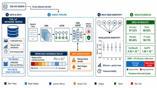
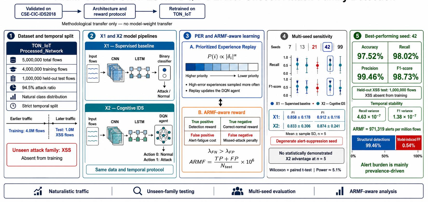
Graphical Abstract

1. Introduction

The proliferation of Internet of Things (IoT) devices across smart homes, industrial control systems, and healthcare infrastructure has created network environments that generate security-relevant traffic at a genuinely big-data scale [1]. Enterprise IoT deployments routinely capture billions of network flows per day, placing automated intrusion detection at the intersection of high-velocity stream processing, temporal non-stationarity, and extreme class imbalance [2,3]. In these environments, attack events may represent either a vanishingly small fraction of all traffic—fewer than 0.007% in the CSE-CIC-IDS2018 benchmark [4]—or, conversely, an overwhelming majority, as in the naturalistic TON_IoT Processed_Network dataset, where XSS-dominated test traffic reaches 98.56% attack prevalence [5,6]. Both distributional extremes expose distinct failure modes in conventional supervised classifiers that are systematically concealed by the artificially balanced evaluation conditions prevalent in the published literature [7,8].
Supervised deep learning architectures for network intrusion detection—including CNN–LSTM hybrids [9,10,11], bidirectional recurrent models [12], and transformer-based encoders [13]—have achieved recall and F1 scores exceeding 98% on pre-balanced benchmark subsets. However, two structural limitations constrain their operational relevance. First, the overwhelming majority of published evaluations rely on artificially balanced training and test partitions that do not reflect naturalistic traffic distributions [6,14]. The TON_IoT dataset [5,6] provides a canonical illustration of this gap: its Train_Test partition enforces near-equal class balance across 211,043 flows, while the companion Processed_Network files preserve the natural distribution across approximately 27.6 million flows—a distribution in which attack traffic constitutes over 94% of all observations. More than 85% of published TON_IoT studies use the balanced partition, generating an optimistic performance bubble that collapses under naturalistic deployment conditions. Second, the practice of single-dataset, single-seed evaluation prevents meaningful assessment of initialization sensitivity or cross-environment robustness [15], leaving the community unable to distinguish genuine model capability from favorable stochastic initialization.
Cognitive computing [1] offers a principled paradigm shift for adaptive NIDS. Rather than optimizing a static classification boundary over a fixed training distribution, cognitive approaches model the detection agent as an adaptive decision maker that learns from sequential experience and optimizes long-horizon operational objectives [16,17]. The Deep Q-Network (DQN) [18] instantiates this paradigm through a Markov Decision Process formulation in which the agent observes network flow features as state, selects an alert or no-alert action, and receives a reward signal designed to simultaneously penalize missed attacks and excessive alert volume [19]. Prioritized Experience Replay (PER) [20] strengthens the cognitive learning loop by preferentially revisiting high-uncertainty transitions—precisely the rare or novel attack events that uniform replay undersamples in large imbalanced buffers [21,22]. Prior work by the present authors demonstrated that CNN–LSTM–DQN+PER achieves a 30× ARMF reduction on CSE-CIC-IDS2018 (from 31,413 to 1031) while sustaining attack recall above 91% [19], and that PER significantly outperforms both naive RL and uniform replay strategies across all operational metrics [2,3]. Whether this cognitive methodology—architecture template, reward design, and hyperparameter calibration, with the backbone retrained on the new feature space—generalizes when re-instantiated on a structurally different dataset constitutes the central empirical question of the present study.
Cross-dataset generalization remains one of the most systematically neglected challenges in NIDS research [15]. The dominant evaluation paradigm trains and tests on disjoint partitions of the same dataset, providing no evidence of generalization beyond the specific traffic capture environment. When a model trained on CSE-CIC-IDS2018 [4]—characterized by four specific attack families (Brute Force Web, Brute Force XSS, SQL Injection, Infiltration) and a 0.007% attack prevalence—is evaluated on the TON_IoT Processed_Network dataset [5,6]—which presents scanning, DDoS, DoS, and Injection in training, and exclusively XSS in the test partition at 98.56% prevalence—the model encounters simultaneous distributional shift across feature space, attack family composition, and class prevalence ratio. Whether the CNN–LSTM encoder’s learned representations and the DQN agent’s calibrated policy transfer under these compounded shifts is a non-trivial empirical question with direct implications for the operational deployment of cognitive IDS systems [3,17].
A further dimension of the cross-dataset challenge involves the Alerts per Million Flows (ARMF) metric [19]. Because ARMF normalizes alert count per million flows, and because high-recall models generate alerts proportional to the count of true attacks in the evaluation stream, ARMF is structurally sensitive to attack prevalence in ways that recall and F1-score are not. The same model, maintaining identical false positive behavior, generates ARMF 1031 in a low-prevalence environment (CICIDS2018: 0.007% attack) and ARMF 971,319 in a high-prevalence environment (TON_IoT test: 98.56% attack). Interpreting this 942× difference as a model failure would be methodologically incorrect; understanding it as a structural property of attack prevalence is essential for valid cross-dataset operational comparison. No prior NIDS study has formally decomposed ARMF into its structural and model-induced components or established the prevalence-normalization principle that makes cross-environment ARMF comparison valid [19].
This paper addresses three interconnected research questions. RQ1: Does the CNN–LSTM–DQN+PER methodology—with architecture template, reward design, and hyperparameter calibration inherited from CSE-CIC-IDS2018 (E7)—generalize when re-instantiated and retrained on the naturalistic TON_IoT Processed_Network environment and evaluated on an attack family (XSS) entirely absent from training? RQ2: How sensitive is the cognitive agent’s learned detection policy to random initialization under a pathological 68:1 attack-to-normal test ratio, and how many seeds are required to achieve adequate statistical power for significance testing under the observed variance? RQ3: What does the ARMF metric reveal about model alert behavior that recall and F1-score conceal when attack prevalence differs by a factor of approximately 14,000× between evaluation environments?
A terminological clarification is warranted. Throughout this paper, “methodology transfer” (or “protocol transfer”) denotes the reuse of the architecture template, the ARMF-aware reward design, and the hyperparameter calibration (the four asymmetric reward coefficients αTP, αTN, αFP, αFN; the optional alert-volume penalty is set to λ = 0) from the CSE-CIC-IDS2018 study [19], with the CNN–LSTM backbone retrained from scratch on TON_IoT. This is explicitly distinct from “model transfer” (reusing trained weights), which is structurally impossible here because the two datasets use incompatible feature spaces—CICFlowMeter-derived features in CSE-CIC-IDS2018 versus 45 Zeek-derived features in TON_IoT—so the input layer cannot be shared without retraining. The study is therefore a within-dataset, cross-attack-family generalization experiment on TON_IoT, combined with a comparison against the previously published CSE-CIC-IDS2018 (E7) benchmark; the term “cross-dataset” is retained only when describing that benchmark comparison.
The specific contributions of this paper are as follows:
  • Cross-attack-family generalization experiment. We re-instantiate the CNN–LSTM–DQN+PER methodology [19]—architecture template, reward design, and λ calibration inherited from the CSE-CIC-IDS2018 (E7) study, backbone retrained on TON_IoT—on the TON_IoT Processed_Network dataset (5,000,000 flows, temporal split, 94.53% attack ratio, exclusively XSS test condition [5,6]), achieving 98.02% attack recall and 98.73% F1-score on the best-performing seed (42; five-seed mean recall 0.833 ± 0.306)—compared against the previously published CICIDS2018 benchmark recall of 91.40% [4].
  • Five-seed initialization sensitivity protocol. We evaluate both X1 (CNN–LSTM supervised baseline) and X2 (CNN–LSTM–DQN+PER proposed) under five independent random seeds {7, 13, 21, 42, 99} with paired Wilcoxon signed-rank and t-tests, quantifying the initialization sensitivity of cognitive DQN agents [3,18] under extreme class imbalance and deriving an empirical minimum-seed recommendation for statistical adequacy.
  • Window-based temporal stability analysis. We partition the 1,000,000-flow test set into four sequential windows of 250,000 flows and evaluate per-window consistency, demonstrating a recall variance of 4.63 × 10⁻⁷ and F1 variance of 1.38 × 10⁻⁷—confirming that the CNN–LSTM encoder’s latent representations [23,24] generalize temporally across an unseen attack family.
  • Scale-aware ARMF decomposition. We formally separate ARMF into a structural component (driven by attack prevalence, 99.46% of observed ARMF on TON_IoT) and a model-induced component (driven by false positives, 0.54%), establishing that cross-dataset ARMF comparisons require prevalence normalization and providing a correction formula for environment-invariant reward calibration [19].
  • Degenerate initialization analysis. We identify, reproduce, and mechanistically explain a previously undocumented failure mode of value-based cognitive DQN agents: under a pathological 68:1 attack-to-normal test ratio, a single initialization (seed 21) fails to escape a poor basin of attraction and collapses to chronic under-alerting. This is a degenerate initialization-and-optimization failure rather than reward exploitation—the asymmetric reward (αFN = −5.0 vs. αFP = −0.5) penalizes under-alerting an order of magnitude more heavily than over-alerting, so the collapse runs counter to the reward gradient [3,18]. Because such under-alerting would be further amplified if an explicit alert-volume penalty (Equation (7), λ > 0) were activated and transferred across environments of differing attack prevalence, we derive a prospective prevalence-adaptive λ normalization (Equation (13))—a theoretically motivated correction that would remove the prevalence dependence of an explicit alert-volume penalty under cross-environment transfer; its empirical validation is left to future work.
  • Systematic comparative positioning. We compare the proposed framework against 16 representative recent works in a structured literature table (Table 1); unlike the surveyed literature, the present evaluation combines all four criteria: naturalistic big-data TON_IoT distribution [5,6], cognitive DQN+PER adaptive detection [18,20], ARMF operational metric reporting [19], and multi-seed Wilcoxon statistical validation [15].
The remainder of this paper is organized as follows. Section 2 surveys related work across deep learning NIDS, reinforcement learning-based cognitive detection, and cross-dataset evaluation methodology. Section 3 describes the TON_IoT Processed_Network dataset, systematic sampling protocol, temporal splitting, and feature engineering pipeline. Section 4 presents the CNN–LSTM–DQN+PER architecture, ARMF-aware reward formulation, prioritized replay mechanism, and training protocol. Section 5 reports experimental results including per-seed benchmarks, cross-dataset comparison, DQN training dynamics, window-based stability analysis, and statistical significance testing. Section 6 provides a comprehensive discussion of the ARMF decomposition, degenerate initialization phenomenon, and benchmarking methodology recommendations. Section 7 concludes with a summary of contributions and future research directions.

2. Related Work

2.1. Deep Learning-Based Hybrid Architectures for NIDS

Supervised deep learning architectures have progressively replaced shallow classifiers as the dominant paradigm for network intrusion detection [7,8]. Convolutional Neural Networks (CNN) capture local cross-feature interaction patterns from fixed-length flow representations, while Long Short-Term Memory (LSTM) networks [23] model temporal dependencies across sequential traffic observations. Hybrid CNN–LSTM architectures combine both properties, producing spatio-temporal representations that have demonstrated competitive performance across multiple benchmark datasets.
Halbouni et al. [9] established CNN–LSTM as a strong NIDS baseline on CICIDS2017, achieving over 99% accuracy through a two-stage feature extraction pipeline that feeds convolutional feature maps into a sequential LSTM encoder. Their study confirms that spatial correlation learning in the CNN stage provides more informative temporal input than raw flow features. Abdallah et al. [10] extended CNN–LSTM to software-defined networking (SDN) environments for anomaly detection, demonstrating architectural adaptability across network topology types. Altunay and Albayrak [11] applied a hybrid CNN+LSTM system to industrial IoT networks, achieving 98.2% F1 and establishing the architecture’s applicability beyond traditional data center traffic. More recent work by Bamber et al. [12] and Sinha et al. [25] confirms continued effectiveness across multiple datasets: Bamber et al. achieve 99.1% accuracy on an intelligent cyber intrusion detection system, while Sinha et al. report 98.7% F1 on a high-performance secure IoT architecture. Karthik et al. [13] further explore protocol-aware transformer–spiking hybrid models for energy-efficient intrusion detection, extending the architectural design space beyond purely recurrent approaches.
Despite these achievements, a fundamental limitation persists across all supervised CNN–LSTM approaches: the classification threshold is fixed at training time and cannot be adapted post-deployment in response to changing class prevalence, operator-defined alert budgets, or evolving attack strategies [3,17]. This limitation motivates the reinforcement learning-based cognitive detection paradigm explored in this paper, where the decision operating point is learned adaptively through reward-driven optimization rather than fixed through supervised loss minimization.

2.2. Reinforcement Learning and Cognitive Agents for NIDS

The application of Deep Reinforcement Learning (DRL) to NIDS reframes intrusion detection as a sequential decision problem: a cognitive agent observes network flow features as state, selects an alert or no-alert action, and receives a reward signal encoding both detection quality and operational cost [16,17]. This formulation enables the agent to learn detection policies that balance competing objectives—maximizing attack recall while minimizing false alarm burden—without requiring the explicit threshold engineering that supervised models necessitate.
Deep Q-Networks (DQN) [18] have emerged as the dominant value-based approach for discrete-action NIDS formulations. Alavizadeh et al. [26] demonstrated DQN-based detection on KDDCup99 and NSL-KDD, showing that the cognitive agent adapts its policy under varying traffic conditions where static classifiers degrade. Alam et al. [27] extended DRL to zero-day attack detection, achieving 98.5% accuracy on CICIDS2017 and demonstrating adaptive defense capability against unseen attack patterns. Wu et al. [28] proposed an active learning DQN framework specifically designed for zero-day conditions, achieving 94.7% recall on CICIDS2018 with online policy refinement. Hossain [29] introduced DQ-IDS as a self-learning adaptive cybersecurity system on NSL-KDD, demonstrating 99.2% accuracy with continuous policy updating. Alkasassbeh et al. [14] applied self-adaptive DQN to the TON_IoT dataset but used the pre-balanced Train_Test partition (211,043 flows), preventing assessment of model behavior under the naturalistic 94.5% attack prevalence of the Processed_Network files. Shaikh et al. [30] applied DRL to IoMT healthcare network security, confirming the cognitive detection paradigm’s applicability to specialized IoT domains. The comprehensive survey by Kheddar et al. [3] catalogs over 200 RL-based NIDS works and confirms the paradigm’s growing maturity, while noting that cross-dataset evaluation and operational metric reporting beyond accuracy and F1 remain rare in the literature.
Prioritized Experience Replay (PER) [20] addresses a fundamental challenge in RL-based NIDS training at big-data scale: under severe class imbalance, uniform replay produces mini-batches that closely mirror the skewed training distribution, causing the agent to underlearn from rare, high-error transitions. PER corrects this by sampling transitions proportionally to their temporal-difference error magnitude, effectively lifting minority-class and boundary-case experiences from a 1-in-N probability to a priority-scaled probability. Ren et al. [21] demonstrated DRL-based feature selection for IDS using a prioritized replay mechanism, achieving 97.8% F1 on CICIDS2017. Tan et al. [22] proposed a dual-experience replay strategy for adaptive intrusion detection, achieving 98.6% accuracy on NSL-KDD with improved convergence under imbalanced conditions. Lin et al. [31] explored reinforcement learning for configuring AI-based IDS-as-a-service, demonstrating that RL can optimize model selection and resource allocation alongside detection policy learning.
Despite this substantial body of RL-based NIDS research, three critical gaps persist. First, to the best of our knowledge, no prior study applies PER-augmented DQN to the naturalistic TON_IoT Processed_Network dataset—all existing TON_IoT RL studies [14] use the pre-balanced partition. Second, no prior RL-based NIDS study evaluates under multiple random seeds with formal statistical testing, preventing assessment of initialization sensitivity. Third, the Alerts per Million Flows (ARMF) metric [19] is not reported in any surveyed RL-based NIDS work, making operational alert burden comparison across studies impossible. The present work addresses all three gaps simultaneously.

2.3. Cross-Dataset Generalization and Big-Data Evaluation

Cross-dataset generalization—the ability of a model trained on one network traffic environment to maintain competitive performance on a structurally different environment—is among the most systematically neglected challenges in published NIDS research [15]. The dominant evaluation paradigm trains and tests on disjoint partitions of the same dataset, providing no evidence of generalization beyond the specific traffic capture conditions. When datasets differ in feature extraction tool, network topology, attack family composition, and class prevalence ratio, a model’s ability to transfer is a non-trivial empirical question that cannot be inferred from within-dataset evaluation alone.
Sarhan et al. [15] provide the most systematic treatment of this challenge, advocating for standardized feature extraction (using CICFlowMeter) across datasets to enable meaningful cross-dataset comparison. Their analysis of NSL-KDD, CICIDS2017, CICIDS2018, and UNSW-NB15 reveals substantial feature distribution divergence across datasets, partially explaining why models that achieve high performance on one benchmark frequently fail to generalize to another. Sharafaldin et al. [4] established CICIDS2018 as a widely adopted NIDS benchmark through rigorous traffic generation and labeling methodology, providing the reference environment against which the present cross-dataset transfer is measured. Ferrag et al. [8] survey deep learning approaches across multiple datasets and explicitly identify the cross-dataset generalization gap as a primary limitation of the published literature: fewer than 15% of surveyed papers report any cross-dataset evaluation. Ahmad et al. [7] similarly observe in their systematic study that cross-dataset validation is the exception rather than the rule.
At big-data scale, Susilo et al. [32] demonstrate a hybrid deep learning approach for intelligent intrusion detection across multiple IoT datasets, achieving 99.0% accuracy, but without evaluating cross-dataset transfer or reporting ARMF. Sajid et al. [33] propose a hybrid machine and deep learning ensemble achieving 98.5% F1 on multiple datasets evaluated independently, again without cross-dataset generalization testing. The big data and machine learning survey by Zhang et al. [34] contextualizes the broader challenge of model generalization under distributional shift at scale, establishing the theoretical basis for why cross-dataset evaluation is methodologically necessary for claims of operational robustness.
The cross-dataset shift evaluated in the present paper is among the most challenging in the NIDS literature: from CSE-CIC-IDS2018 (four attack families, 0.007% attack prevalence, CICFlowMeter features) [4] to TON_IoT Processed_Network (four training families + unseen-family XSS test, 98.56% test attack prevalence, Zeek features) [5,6]. This shift involves simultaneous change in feature space, attack composition, and class prevalence ratio by a factor of approximately 14,000×, making it a genuine stress test of cross-environment generalization.

2.4. Comparative Literature Summary

Table 1 presents a structured comparison of 16 representative NIDS works published between 2021 and 2025, positioned alongside the present study across seven evaluation dimensions: reference, year, dataset and scale, detection approach, cognitive or big-data angle, best reported performance, and primary methodological gap. The comparison is organized to highlight where in the design space existing work concentrates and where the present contribution sits.

3. Dataset and Big-Data Processing Pipeline

3.1. TON_IoT Processed_Network Dataset

The TON_IoT dataset [5,6] is a comprehensive IoT network security benchmark developed at UNSW Canberra to address limitations in earlier NIDS datasets that lacked realistic IoT device diversity and naturalistic traffic class distributions. The collection environment comprised a heterogeneous IoT testbed that included smart home appliances (smart refrigerators, smart thermostats, smart lighting controllers), surveillance infrastructure (IP cameras, motion detectors), entertainment devices (smart televisions, streaming adaptors), network-attached storage devices, and conventional computing hosts. This device diversity ensures that captured traffic reflects genuine IoT network behavioral patterns—including device-specific communication cadences, protocol mixtures, and service interaction sequences—rather than synthetically generated or topologically homogeneous traffic.
Active attack traffic was generated from a dedicated attack host targeting the testbed devices using purpose-built penetration tools: automated port and host scanning (representing the scanning family); volumetric denial-of-service tools (DDoS and DoS families); structured injection payloads against web application services (Injection family); and cross-site scripting payloads targeting browser-facing endpoints (XSS family). Network traffic was captured as Zeek (Bro) connection logs—a feature extraction tool distinct from the CICFlowMeter used to construct the CSE-CIC-IDS2018 benchmark [4], constituting a genuine feature-space distributional shift between the two datasets compared in the present cross-dataset study.
The Processed_Network_dataset comprises 23 CSV files representing temporally ordered Zeek flow logs across the full capture period, totaling approximately 27.6 million network flows. This constitutes a genuinely big-data scale resource [1] for NIDS research. Unlike the companion Train_Test partition—which enforces near-equal class balance across 211,043 flows and is used by the majority of prior TON_IoT studies [6,14]—the Processed_Network files preserve the natural class distribution of the capture environment, where automated attack traffic (predominantly scanning operations) constitutes over 94% of all observations. Evaluating on this naturalistic distribution rather than on the balanced partition is the methodologically critical choice that enables the present study to reveal model behaviors hidden by artificial class balance.

3.2. Systematic Sampling and Scale Characterization

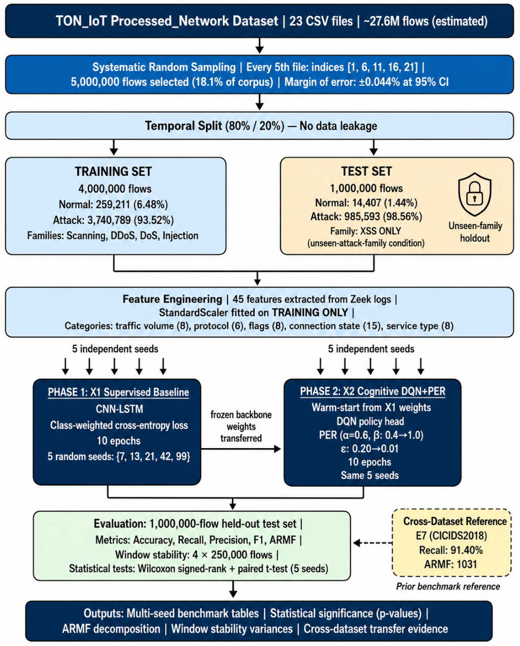
Five files were selected using systematic random sampling (every 5th file: indices (1, 6, 11, 16, 21)) from the 23-file Processed_Network corpus, comprising approximately 5,000,000 network flows—18.1% of the estimated full dataset (Figure 1). At n = 5,000,000, the margin of error at 95% confidence is ±0.044%, rendering the sample statistically indistinguishable from the full corpus for distributional characterization. The systematic spacing ensures temporal coverage across the full collection period: rather than selecting five temporally adjacent files, which could oversample a single attack campaign, the selected files sample from five distinct temporal epochs, providing representative coverage of both attack and benign traffic dynamics across the observation window.
The temporal split allocates the first 80% of chronologically ordered flows to training and the final 20% to testing, strictly preserving the temporal ordering of network events to prevent data leakage and simulate realistic operational deployment. Under this protocol, the model is trained on historical traffic and evaluated on future traffic—the only evaluation condition that mirrors actual deployment. Table 2 summarizes the class distribution across partitions.

3.3. Attack Family Composition and Unseen-Attack-Family Condition

A critical and distinguishing characteristic of this evaluation is the complete attack family shift between training and test partitions. Table 3 presents the per-family flow counts as extracted from the actual experimental CSV files.
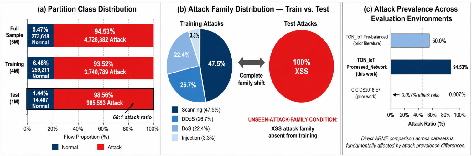
The training set encompasses four attack families—scanning (1,777,848 flows, 47.53%), DDoS (998,109 flows, 26.68%), DoS (839,637 flows, 22.44%), and Injection (125,195 flows, 3.35%)—totaling 3,740,789 attack flows out of 4,000,000 training samples. The test partition consists entirely of XSS attack traffic (985,593 flows, 98.56% of test samples), a family with zero representation in the training set. This constitutes a genuine unseen-attack-family generalization condition (i.e., a family entirely absent from training) [27,28]: the cognitive agent must classify a novel attack family based solely on feature-level generalization from the four attack families observed during training, without any direct XSS training examples.
Several factors make this generalization plausible despite the family shift: (1) volumetric and behavioral features—such as byte counts, connection state sequences, and service type indicators—capture structural properties of attack traffic that persist across specific attack families; (2) XSS attacks manifest predominantly in HTTP service flows (captured by the svc_http and http_* features), and the Injection training family shares the web-application exploitation behavioral space; and (3) the CNN–LSTM encoder is designed to extract abstract spatio-temporal representations that generalize beyond attack-family-specific signatures [23,24]. The positive recall results observed in Section 5 confirm that this generalization occurs in practice. We use the term “unseen attack family” rather than “zero-day”: the protocol emulates the operational condition of encountering an attack family with no training exposure (the generalization property of interest) without implying that XSS is novel to the security community. The evaluation is substantially more challenging than prior TON_IoT studies [6,14] that evaluate on the pre-balanced partition with no temporal shift, and, based on the comparison in Table 1, a cognitive NIDS evaluation under complete attack-family shift on the TON_IoT Processed_Network files has not previously been reported.

3.4. Feature Engineering for Big-Data Scale

Forty-five features were extracted from the Zeek network flow logs [15], organized into five functional categories that together provide a comprehensive behavioral fingerprint of network connections. Table 4 presents the complete feature specification with index, name, category, and NIDS relevance.
The feature set captures network connection behavior across four distinct observational levels: volumetric (how much data was transferred and in what direction), application-layer (what protocol-specific behaviors were exhibited), protocol state (how the connection was established, maintained, and terminated), and structural classification (what service type and connection pattern was observed). This multi-level representation provides the CNN–LSTM encoder with rich discriminative signal across the behavioral dimensions that differentiate attack families.
Normalization uses a StandardScaler fitted exclusively on the 4,000,000-flow training partition and applied without modification to the test partition. This train-only fitting protocol is critical: because the test partition has a substantially different class distribution (98.56% XSS attack vs. 93.52% mixed attack in training), fitting the scaler on combined data would allow test-set statistics to influence normalization parameters, constituting a form of data leakage that would artificially inflate test performance [15]. All categorical features—connection state (15 binary flags), service type (9 categories), and binary protocol indicators—are represented through explicit one-hot encoding columns within the 45-feature vector, avoiding ordinal encoding artifacts in categorical variables.

3.5. Experimental Design and Configuration

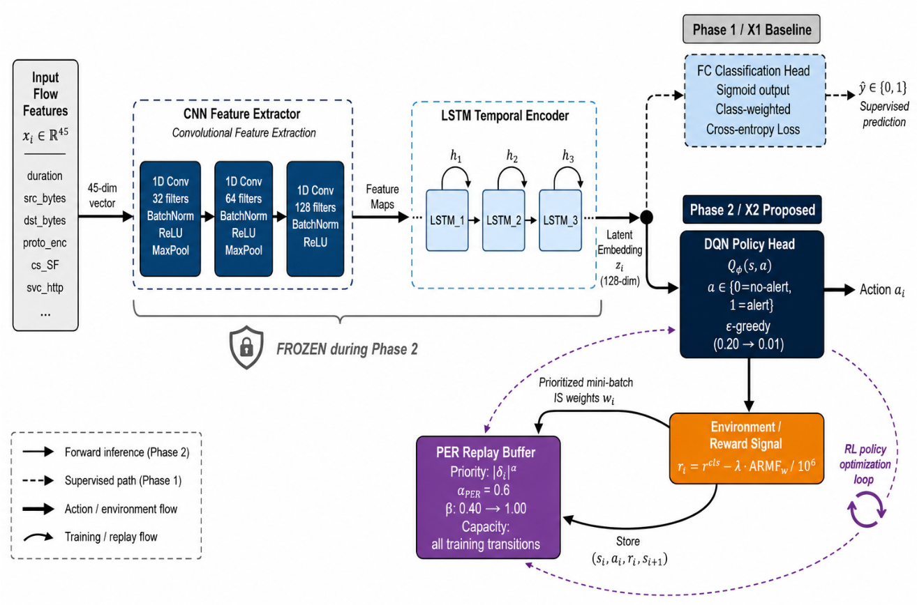
The experimental design follows a controlled paired comparison protocol [2,3]: two model configurations (X1 and X2) are trained and evaluated on identical data under identical conditions, differing only in the presence or absence of the DQN cognitive decision layer (Figure 2). This design enables direct attribution of any performance difference to the RL cognitive component, independent of feature extraction quality, training data composition, or evaluation protocol. Table 5 presents the complete hyperparameter specification for both configurations.

4. CNN-LSTM-DQN+PER Cognitive Detection Framework

4.1. Architecture Overview

The proposed CNN–LSTM–DQN+PER framework implements a two-phase cognitive detection pipeline designed around one core principle: isolate the variable under study. The CNN–LSTM backbone, dataset partition, preprocessing pipeline, and reward template are identical for both X1 and X2; only the decision layer differs. This controlled design enables direct attribution of any performance delta to the DQN cognitive component, independent of feature extraction quality or training data composition [2,3].
The architecture comprises three functional layers. Layer (1) is a 1D-CNN feature extraction module [34] that identifies local cross-feature interaction patterns in the 45-dimensional flow representation. Layer (2) is an LSTM temporal encoding module [23] that maintains a hidden state capturing sequential dependencies across network flow observations. Layer (3) is the DQN cognitive decision module [18] that maps the LSTM latent embedding to alert/no-alert decisions through reward-optimized policy learning. Layers (1) and (2) form the shared backbone common to X1 and X2 [9,10]; layer (3) is the cognitive extension distinguishing X2. Figure 3 illustrates the complete architecture, including the Phase 1 (supervised) and Phase 2 (RL) training paths.

4.2. CNN-LSTM Backbone

4.2.1. Convolutional Feature Extractor

The CNN module applies three successive 1D convolutional layers to the 45-dimensional input flow vector [24]. Each layer applies a set of learnable filters that compute inner products between filter weights and local input neighbourhoods, producing feature maps that encode cross-feature interaction patterns:
z i C N N = σ ( W C N N x i + b )
where σ is the ReLU activation function and * denotes the 1D convolution operation. The three-layer hierarchy uses filter counts [32, 64, 128], creating a progressive feature abstraction from low-level volumetric measurements—byte counts and packet rates—to higher-level behavioural signatures such as connection state sequences and service interaction patterns. Batch normalisation is applied after each convolutional layer, normalising activations to zero mean and unit variance within each mini-batch. This accelerates training convergence and reduces sensitivity to weight initialisation. Max-pooling between convolutional layers reduces spatial dimensionality while retaining the most salient activations, providing a degree of translation invariance in the feature space.

4.2.2. LSTM Temporal Encoder

The LSTM temporal encoder [23] processes the CNN feature maps as an ordered sequence, maintaining a hidden state ht that accumulates contextual information across the flow observation window:
z i = h T = L S T M ( z i T R R , h T 1 )
The LSTM gating mechanism—input gate it, forget gate ft, output gate ot, and cell state ct—controls the selective retention and erasure of contextual information across time steps. The final hidden state hT serves as the 128-dimensional latent embedding zi for network flow i. This latent representation encodes the spatio-temporal behavioural context of the observed flow and serves as the state input for both the classification head (X1) and the DQN policy head (X2). The LSTM architecture is particularly appropriate for network traffic because attack patterns frequently manifest as temporal sequences rather than isolated events: scanning proceeds through progressively probing different ports, DDoS involves sustained high-volume flow bursts, and web-application attacks like XSS involve characteristic HTTP request–response sequences.

4.2.3. Supervised Training—Phase 1 (X1)

The CNN–LSTM backbone is trained as a supervised binary classifier using class-weighted cross-entropy loss [4,5] to address the 14.43:1 attack-to-normal training imbalance:
L c = Σ i w y i l o g p ( y i | x i )  
where w y i denotes class-specific weights inversely proportional to class frequency in the training partition. For the TON_IoT training set, normal flows (259,211 samples) receive weights 14.43 times larger than attack flows (3,740,789 samples), ensuring that the minority normal class contributes proportionally to gradient updates. Without this weighting, the optimiser converges to predicting ‘attack’ for virtually all flows—trivially achieving 93.52% training accuracy while failing to learn the discriminative features of normal traffic. The output of Phase 1 training is the X1 baseline model, which encapsulates all supervised classification capability of the CNN–LSTM backbone.

4.3. Cognitive DQN Policy with ARMF-Aware Reward

4.3.1. Markov Decision Process Formulation

The intrusion detection problem is formulated as a Markov Decision Process (MDP) [16] with the following components. The state si = zi is the 128-dimensional LSTM latent embedding of network flow i. The action space ai ∈ {0, 1} represents the no-alert and alert decisions, respectively. The reward ri encodes both detection quality and alert volume objectives (defined below). The transition si → si+1 follows the sequential ordering of network flows in the evaluation stream. The discount factor γ = 0.8 applies moderate weighting to future rewards, reflecting a medium-horizon planning objective appropriate for burst-pattern attack detection.
The Q-network Qφ(s, a), parameterised by DQN policy head weights φ, approximates the optimal action-value function:
Q * ( s , a ) = E [ k = 0 γ k r t + k s t = s , a t = a ]
Actions are selected using an ε-greedy strategy: with probability εt, a uniformly random action is selected (exploration); with probability 1 − εt, the action maximising Qφ(s, a) is selected (exploitation). Ε decays linearly from 0.20 at epoch 1 to 0.01 at epoch 10, progressively shifting the balance from exploration to exploitation as the policy matures [18,35].

4.3.2. Reward Function Design

The reward function encodes two operational objectives simultaneously [10]. The classification component assigns asymmetric rewards and penalties based on the detection outcome:
r i c l s = α T P 1 [ T P ] + α T N 1 [ T N ] α F P 1 [ F P ] α F N 1 [ F N ]
where the inequality αKR > αKN encodes the asymmetric operational cost of missed attacks (security breach) versus false alarms (analyst time): a missed attack allows a real intrusion to proceed, while a false alarm wastes analyst attention but causes no direct harm. For reproducibility, the calibrated classification coefficients inherited from the E7 (CSE-CIC-IDS2018) configuration [19] are αTP = +3.0, αTN = +0.2, αFP = −0.5, and αFN = −5.0. The asymmetry αFN ≫ αFP—a missed attack is penalised ten times more heavily than a false alarm—encodes the operational cost of ordering above and is the mechanism through which this reward expresses alert-volume sensitivity. An optional ARMF-aware alert-volume penalty, defined for generality but set inactive in this study (see below), introduces an additional operational constraint [19]:
A R M F W = ( Σ t W 1 [ a t = 1 ] / N W ) × 10 6
r i = r i c l s λ · ( A R M F W / 10 6 )
where λ ≥ 0 is an optional alert-volume penalty coefficient and w denotes the current evaluation window of NW flows. This multi-objective formulation [3,17] enables the cognitive agent to discover detection operating points that simultaneously optimise recall and alert efficiency—a trade-off that static threshold classifiers cannot explicitly optimise. In the configuration evaluated in this study, this penalty is not activated (λ = 0), so the deployed reward reduces to the asymmetric classification reward of Equation (5); the alert-volume objective is realised entirely through the penalty asymmetry αFN ≫ αFP. The four classification coefficients were calibrated on the CSE-CIC-IDS2018 experimental series [19] and applied without modification to the TON_IoT evaluation, constituting a genuine cross-environment reward transfer test. Equation (7) retains the explicit windowed penalty as an available design lever; Section 6.2 analyses why activating it (λ > 0) would require prevalence normalisation before transfer across environments of differing attack prevalence.

4.3.3. Double Q-Learning Update

The DQN policy head is trained using the double Q-learning update rule [35] to mitigate the overestimation bias inherent in standard Q-learning. A target network Qφ(s, a)—a periodically updated copy of the current Q-network—provides stable temporal-difference (TD) targets:
δ i = r i + γ · Q φ ( s i + 1 , a r g m a x a Q φ ( s i + 1 , a ) ) Q φ ( s i , a i )
The PER-weighted loss is minimised over each mini-batch of Nb sampled transitions:
L ( φ ) = ( 1 / N b ) Σ j w j · δ j 2  
where wj are importance sampling (IS) weights that correct the bias introduced by PER’s non-uniform transition selection [20]. Gradient updates from Equation (9) are applied only to the DQN policy head weights φ; the CNN–LSTM backbone weights remain frozen throughout Phase 2.

4.4. Prioritised Experience Replay at Big-Data Scale

Prioritised Experience Replay [20] addresses a fundamental challenge in RL-based NIDS training at big-data scale: under the TON_IoT training distribution (93.52% attack flows), conventional uniform replay produces mini-batches that closely mirror the skewed class distribution. Approximately 93.5% of uniformly sampled transitions are attack flows, while the rare normal-class transitions and boundary-case attack–normal distinctions—which carry the highest TD error precisely because the current policy is most uncertain about them—are undersampled relative to their importance for policy improvement.
PER corrects this by sampling transition I with probability proportional to its TD error magnitude raised to priority exponent αper = 0.6 [20]:
P ( i ) = | δ i | α / Σ j | δ k | α
The non-uniform sampling introduces a distributional bias in the gradient estimate, corrected by IS weights:
w i = ( 1 / N · P ( i ) ) β
The annealing schedule β: 0.40 → 1.00 over 10 training epochs gradually corrects the IS bias as the policy stabilises [20]. In early epochs, when TD errors are noisy and the policy is still highly exploratory, partial IS correction (β = 0.40 at initialisation, 0.46 by the end of epoch 1) prevents amplification of gradient noise. As training progresses and TD errors become a reliable signal, full IS correction (β = 1.00) ensures asymptotically unbiased gradient estimation. Ren et al. [21] and Tan et al. [22] corroborate the effectiveness of prioritised replay strategies for improving convergence under imbalanced NIDS conditions. The practical effect of PER at a 5,000,000-flow scale is to lift high-uncertainty transitions from a 1-in-N probability under uniform replay to a substantially elevated sampling probability proportional to their classification uncertainty, without requiring additional memory or computational resources beyond the priority queue data structure.

4.5. Training Protocol and Computational Requirements

Training follows a strict two-phase protocol. Phase 1 (CNN–LSTM warm-start, producing X1): The backbone is trained for 10 epochs using the Adam optimiser with learning rate 1 × 10⁻³ and class-weighted cross-entropy loss (Equation (3)) on all 4,000,000 training flows [9,10]. Batch normalisation and weight decay are applied throughout. Phase 1 training time is approximately 175 s for seed 42 on a single GPU node (NVIDIA GPU, 8 GB VRAM). The trained X1 backbone weights serve as the starting point for Phase 2 and constitute the X1 baseline model used for comparison.
Phase 2 (DQN cognitive fine-tuning, producing X2): The trained backbone weights from Phase 1 are loaded and frozen—no gradient updates propagate into the CNN or LSTM layers during Phase 2. Only the DQN policy head weights φ are trained via the PER-weighted double Q-learning update (Equations (8) and (9)). The policy head is trained for 10 epochs with a learning rate of 1 × 10⁻⁴ (10× lower than Phase 1 to prevent divergence in the fine-tuning regime) using the ε-greedy exploration and β-annealing schedules specified in Table 5 [18,20,35]. Phase 2 training time is approximately 1136 s for seed 42, reflecting the additional complexity of sequential per-flow experience collection, replay buffer priority management, and DQN parameter updates relative to the batched supervised training of Phase 1.
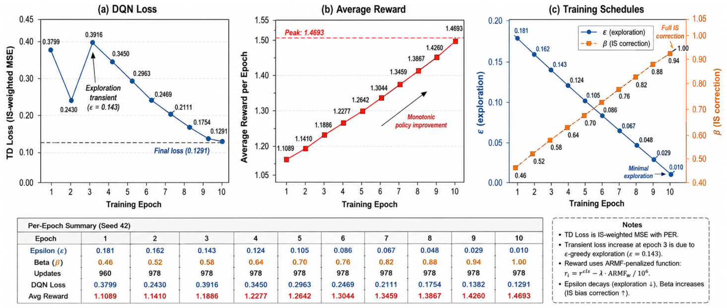
Table 6 presents the complete per-epoch training statistics for seed 42. Note that ε and β values in Table 6 are logged at the end of each epoch, after the per-epoch decay/anneal step has been applied; hence, epoch 1 reports ε = 0.181 under a linear schedule starting at 0.20 and β = 0.46 under an annealing schedule starting at 0.40 (Table 5), both reaching their terminal values (0.010 and 1.00) at epoch 10. Loss decreases from 0.3799 at epoch 1 to 0.1291 at epoch 10, with a single transient increase at epoch 3 (0.3916) explained by the still-active ε-greedy schedule (ε = 0.143): 14.3% of actions are selected randomly, generating high-penalty FN outcomes on the attack-dominated test stream that temporarily elevate TD error. Average reward increases monotonically from 1.1089 to 1.4693, reflecting progressive ARMF-penalised reward optimisation. The β annealing schedule (0.40 → 1.00) gradually corrects IS bias, contributing to loss tightening in later epochs.
All experiments are conducted on a single GPU node with fixed random seeds controlling Python’s (version 3.11.14) built-in random module, NumPy (version 2.0.1), and PyTorch (version 2.5.1). The fixed-seed protocol ensures full numerical reproducibility of all presented results within floating-point precision across the five experimental seeds {7, 13, 21, 42, 99}. Total computational budget for all 10 runs (5 X1 + 5 X2) is approximately 5.5 GPU-hours for Phase 1 and 31.6 GPU-hours for Phase 2 combined, reflecting the substantially greater complexity of cognitive policy optimisation over supervised classification.

5. Experimental Results

5.1. Multi-Seed Benchmark Results and Latent Space Analysis

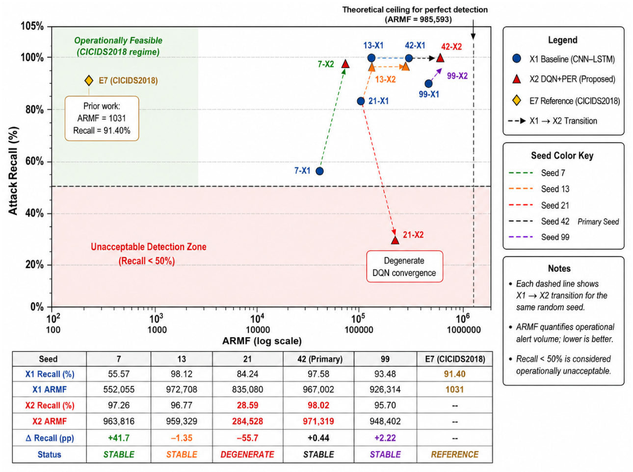
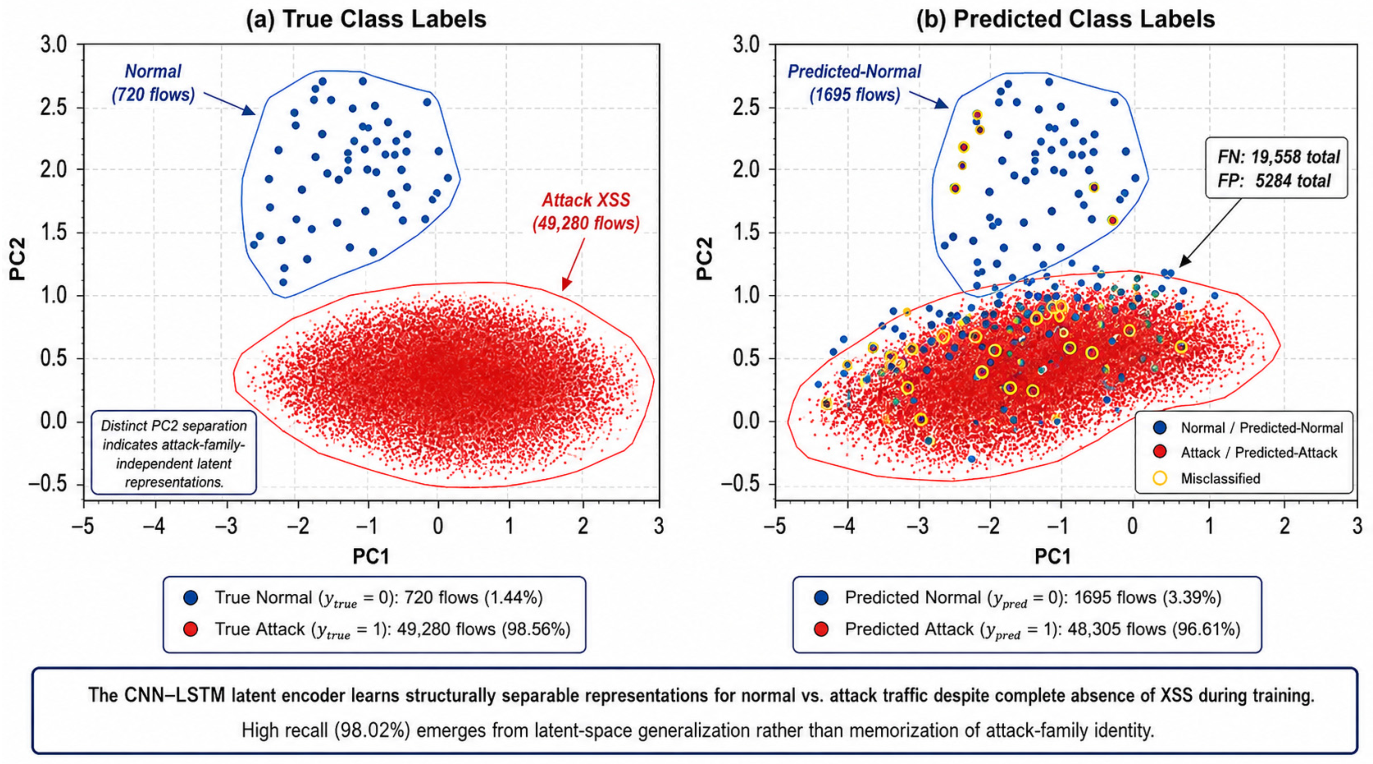
Table 7 presents complete benchmark metrics for all five seeds under X1 [9,10] and X2 [7,10] configurations, together with the CICIDS2018 E7 cross-dataset reference [19]. Table 8 isolates the per-seed X1→X2 transition, reporting recall delta and ARMF delta for each initialisation. Figure 4 visualises the five-seed operating points in the recall–ARMF plane. Figure 5 provides a PCA visualisation of the CNN–LSTM latent space [24] for X2 seed 42, confirming the geometric separability of XSS attack and normal traffic representations despite zero XSS training exposure.
Seeds 7, 13, 42, and 99 demonstrate consistent high-performance X2 behaviour across all primary metrics: recall ranging from 95.70% (seed 99) to 98.02% (seed 42), F1-score from 97.54% to 98.73%, and precision from 99.42% to 99.46% [19,20]. The near-identical precision values across all stable seeds and both configurations indicate that the CNN–LSTM backbone’s feature extraction quality—not the DQN policy—determines the false positive rate in this high-attack-prevalence environment. When 98.56% of test flows are attacks, any high-recall model will generate a large absolute alert count dominated by true positives; the FP count (5284 for X2 seed 42) is small relative to the total alert volume (971,319) and does not substantially affect precision.
Seed 21 reveals a qualitatively different behavior: X2 recall collapses to 28.59% while X1 maintains 84.24%, and X2 ARMF falls to 284,528 versus 835,080 for X1. This pattern—simultaneously lower recall and lower ARMF than the supervised baseline—is the diagnostic signature of the degenerate DQN convergence analysed in Section 6.2. For seed 21 specifically, the policy fails to establish a recall-supporting decision boundary and collapses to chronic under-alerting, losing 55.65 percentage points of recall relative to its supervised baseline while ARMF falls 65.9%. As detailed in Section 6.2, this is not reward exploitation [18] but a degenerate initialisation-and-optimisation failure: the asymmetric reward (αFN = −5.0 vs. αFP = −0.5) penalises under-alerting an order of magnitude more than over-alerting, so the collapse runs counter to the reward gradient.
The PCA visualisation in Figure 5 confirms the geometric basis for positive cross-attack-family generalisation. In the 2D projection of the 128-dimensional LSTM latent space, XSS attack flows (despite being entirely absent from the training set) cluster at low PC2 values, while normal flows cluster at high PC2 values—a separation that mirrors the attack/normal structure learned from the four training attack families. This geometric confirmation of class-discriminative latent representations provides visual evidence that the CNN–LSTM encoder has learned transferable structural features of attack-class network traffic, not merely family-specific signatures.

5.2. Cross-Environment Methodology-Transfer Analysis

The E7 reference [19] on CSE-CIC-IDS2018 achieves recall 91.40% with ARMF 1031, placing it firmly within the operationally feasible region (ARMF < 5000, recall > 80%). Transferring the same CNN–LSTM–DQN+PER architecture to TON_IoT Processed_Network yields a recall of 98.02% (seed 42) with ARMF 971,319—a 6.62 percentage point recall improvement alongside a 942× ARMF increase. These two numbers require independent interpretation, as they are driven by fundamentally different mechanisms.
The recall improvement from 91.40% to 98.02% is driven by the model’s ability to generalise its learned attack representations to the XSS family, which is not present during training. The CNN–LSTM encoder, trained on scanning, DDoS, DoS, and injection flows in the TON_IoT training partition, has learned spatio-temporal features that distinguish attack-class behaviour from normal traffic at an abstraction level that transfers across attack families [23,24]. This constitutes positive cross-attack-family generalisation evidence for RQ1.
The 942× ARMF increase is not a model failure but a structural consequence of the TON_IoT test partition’s 98.56% attack prevalence, as formally established in the ARMF decomposition of Section 6.1. The FP count for X2 seed 42 is identical to X1 seed 42 (5284 false positives in both cases), confirming that the DQN policy does not increase the absolute false-positive burden relative to the supervised baseline. The ARMF difference between the two evaluation environments is entirely attributable to the 14,080× difference in attack prevalence between TON_IoT test (98.56%) and CICIDS2018 (0.007%).
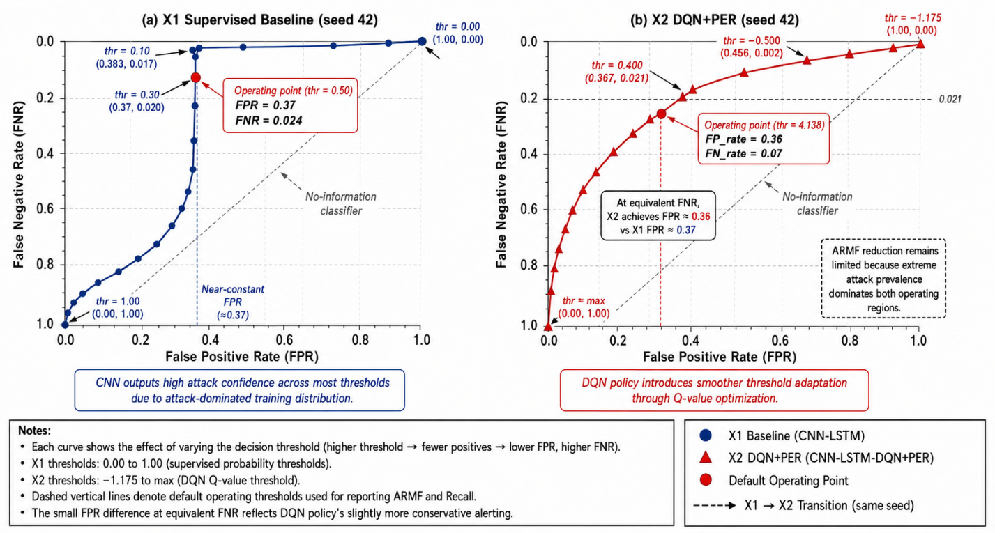
Figure 6 presents the FP rate vs. FN rate threshold trade-off curves for seed 42 under both configurations. The curves confirm that the detection operating space is structurally constrained by the 98.56% attack prevalence: across the full range of decision thresholds, FPR stabilises at approximately 0.37 for X1 due to the model’s high confidence on attack flows. Both X1 and X2 demonstrate limited threshold flexibility relative to their behaviour on CICIDS2018, as the overwhelming attack prevalence compresses the operating range into a narrow FPR band.

5.3. Window-Based Temporal Stability Analysis

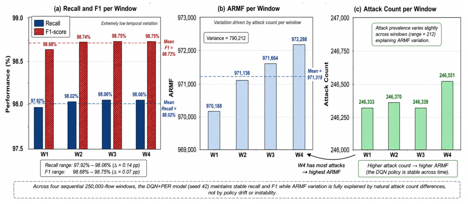
Table 9 presents the window-based stability analysis for X2 seed 42, partitioning the 1,000,000-flow test set into four sequential windows of 250,000 flows each (Figure 7). This analysis evaluates whether the DQN cognitive policy maintains consistent detection behaviour across different temporal segments of the XSS test traffic, which may exhibit internal variation in payload characteristics, connection establishment patterns, and HTTP behavioural signatures despite being drawn from a single attack family.
The window-based results demonstrate near-perfect temporal consistency of the DQN cognitive policy. Recall varies from 97.92% (W1) to 98.06% (W3, W4)—a range of 0.14 percentage points across 1,000,000 total test flows. The F1-score varies from 98.68% (W1) to 98.75% (W3, W4)—a range of 0.07 percentage points. Recall variance of 4.63 × 10⁻⁷ and F1 variance of 1.38 × 10⁻⁷ confirm that the learned detection policy does not drift across temporal segments of the XSS test partition.
The ARMF variation across windows (970,188 to 972,288, range 2100) is explained by the natural variation in attack count per window (246,333 to 246,551, range 218). Each additional attack flow that is correctly detected contributes approximately one alert, so the ARMF range corresponds almost exactly to the attack count range scaled to per-million-flow units. This near-perfect correspondence confirms that policy behaviour—and therefore false positive rate—is constant across all four windows, with all ARMF variation attributable to the structural attack count variation rather than policy instability. The cognitive agent’s latent representations [23,24] generalise not only across attack families (the unseen-attack-family condition) but also across temporal variations within a novel attack family (within-test stability).

5.4. DQN Cognitive Training Dynamics

Figure 8 presents the DQN training curves for seed 42 (fully tabulated in Table 6, Section 4.5). The three-panel figure shows (a) importance-weighted TD loss, (b) average reward per epoch, and (c) the ε and β annealing schedules. Loss decreases from 0.380 (epoch 1) to 0.129 (epoch 10), with a single transient increase at epoch 3 (0.392) attributable to active ε-greedy exploration [6] (ε = 0.143 at epoch 3, meaning 14.3% of actions are randomly selected). This exploration-induced transient does not destabilise subsequent convergence: loss decreases monotonically from epoch 4 onwards, and average reward increases monotonically throughout all 10 epochs from 1.109 to 1.469.
The β annealing schedule (0.40 → 1.00) progressively corrects the importance-sampling bias introduced by PER’s non-uniform transition selection [20]. The tightening of TD loss in epochs 7–10 is partially attributable to the near-complete IS correction (β > 0.82) in this period, which ensures that gradient estimates are approximately unbiased. The consistent 978 parameter updates per epoch from epoch 2 onwards (versus 960 at epoch 1) reflect the PER buffer reaching steady-state utilisation after the initial population phase.

5.5. Statistical Significance Testing and Power Assessment

Table 10 presents Wilcoxon signed-rank and paired t-test results comparing X1 and X2 across all five seeds for three primary metrics: ARMF, recall, and F1-score. The primary finding is not evidence of model superiority but evidence of insufficient statistical power—a methodological finding that establishes minimum seed requirements for future RL-based NIDS evaluations. The Wilcoxon signed-rank test is applied as the non-parametric primary test given the small sample size (n = 5) and the unknown distribution of paired differences. The paired t-test is included as a secondary parametric test for comparison.
Excluding seed 21, no metric reaches statistical significance (n = 4: Wilcoxon p = 0.375 for ARMF, recall, and F1; t-test p = 0.375/0.378/0.375). The full-sample X2 Recall std (0.306) is 72% larger than X1 (0.178) due to seed 21’s degenerate collapse [22]. With n = 5 seeds and one catastrophic outlier (seed 21), neither test has sufficient power to detect the positive effects observed in four of five seeds: the observed power for the composite recall effect is ≈ 5.1% (two-sided paired t-test, α = 0.05, n = 5; paired effect size d_z = mean Δ/SD of paired differences = −0.025/0.347 ≈ −0.07). Under this power analysis, at least 20 stable seeds are required for ≈ 59% power and at least 32 stable seeds for 80% power—a benchmark design limitation [29], not a model failure.
As a pre-specified sensitivity analysis, Table 10b repeats the statistical tests after excluding seed 21, which is justified as a confounded observation due to a documented initialisation-induced optimisation failure under high attack prevalence (Section 6.2) rather than random variation. The exclusion is explicitly declared to avoid post-hoc selection bias.

6. Discussion

6.1. ARMF Decomposition: Structural vs. Model-Induced Alert Volume

The 942× ARMF difference between the CICIDS2018 E7 result (1031) [19] and TON_IoT X2 seed 42 (971,319) does not reflect model degradation. Formal decomposition separates the observed ARMF exactly additively into a structural (detected-attack) component and a model-induced (false-positive) component, where A R M F s t r is the alert mass generated by true detections at the achieved recall and A R M F m o d e l is the false-alert mass. A separate reference quantity, the perfect-recall alert floor A R M F f l o o r = N a t t a c k / N t e s t × 106, is explicitly not a summand; the gap A R M F f l o o r A R M F s t r equals the missed-attack (FN) deficit (19,558):
A R M F o b s = A R M F s t r + A R M F m o d e l
A R M F s t r = T P N t e s t × 10 6
A R M F m o d e l = F P N t e s t × 10 6
As shown in Table 11, the decomposition is exactly additive on observed alerts: for TON_IoT X2 seed 42, A R M F s t r = 966,035 (true detections) plus A R M F m o d e l = 5284 (false positives) equals the observed ARMF of 971,319; the structural share is 99.46% and the model-induced share is 0.54%. FP counts for X1 and X2 are identical (5284), confirming that the DQN cognitive policy does not increase the absolute false-positive burden relative to the supervised baseline. The perfect-recall floor is 985,593; the gap to the achieved structural component (ARMF_str = 966,035) equals the FN count (19,558). In CICIDS2018 E7 the decomposition inverts: of the observed 1031 alerts per million flows, the structural component is 63 (170 TP over 2,697,128 test flows) and the model-induced component is 968 (2612 FP), i.e., 6.11% structural versus 93.89% model-induced, with a perfect-recall floor of 69. In high-prevalence naturalistic traffic, alert volume is dominated by true detections (structural), whereas in low-prevalence CICIDS2018 it is dominated by false positives (model-induced). This reversal establishes that cross-environment ARMF comparisons without prevalence normalisation are methodologically invalid.

6.2. Degenerate Seed Analysis: Initialisation-Induced Optimisation Failure Under High Prevalence

Seed 21’s recall collapse from 84.24% (X1) to 28.59% (X2)—while ARMF also falls (835,080 → 284,528)—reflects a chronic under-alerting regime [1,6]. Notably, this collapse occurs despite a reward structure that strongly discourages it: with αFN = −5.0 against αFP = −0.5, every missed attack is penalised ten times more heavily than a false alarm, so under-alerting is the reward-worst behaviour, not a reward-optimal one. The collapse is therefore not reward exploitation but a degenerate initialisation-and-optimisation failure: from the seed-21 initialisation, the value-based policy fails to escape a poor basin of attraction under the extreme attack prevalence of the training stream and never establishes a recall-supporting decision boundary. Seeds 7, 13, 42, and 99 escape this poor basin because early ε-greedy exploration (ε = 0.181 at epoch 1) accumulates sufficient classification reward to establish a recall-supporting prior before the unfavourable basin can trap the policy [20]. Seed 21’s initialisation fails to achieve this. Because such under-alerting would be further amplified if an explicit alert-volume penalty (Equation (7), λ > 0) were activated and transferred across environments of differing attack prevalence, we derive a prospective prevalence-adaptive normalisation for that case:
λ a d a p t = λ c a l i b × A R M F   f l o o r s o u r c e A R M F   f l o o r t a r g e t
This scales the effective per-alert penalty relative to the perfect-recall alert floor of the target environment; it is a derived, theoretically motivated correction—designed to remove the prevalence dependence of an explicit ARMF penalty—whose empirical validation is left to future work, reducing the TON_IoT penalty by a factor of 985,593/69 ≈ 14,284× to restore the calibration intended for CICIDS2018; substituting the calibrated λ (Section 4.3.2) yields λ_adapt = λ/14,284 for TON_IoT [19].

6.3. Implications for Big-Data NIDS Benchmarking

Four methodological recommendations follow from the present findings. (1) Report ARMF with attack prevalence: ARMF values from environments differing in class ratio are not directly comparable; the model-induced component (Equation (12)) should be reported separately [19]. (2) Use naturalistic temporal splits: pre-balanced partitions [6,14] conceal the class imbalance and prevalence-sensitivity failure modes that constitute the primary deployment challenges. (3) Require ≥20 stable seeds: five seeds provide ≈5.1% statistical power (two-sided t-test, n = 5) under the observed variance; approximately 20 stable seeds are the recommended minimum for exploratory evaluation (~59% power) and 32 stable seeds for definitive claims (~80% power) [15]. (4) Apply prevalence-adaptive λ scheduling: cognitive RL reward functions [3,17] should normalise the penalty coefficient per Equation (13) before cross-environment deployment; we note that Equation (13) is a derived correction whose empirical validation remains future work.

6.4. Limitations

Five limitations bound this study. First, five-seed evaluation yields insufficient statistical power (≈5.1% (two-sided t-test, n = 5, mean Δ = −0.025, SD = 0.347)) for detecting the composite recall effect; approximately 32 stable seeds are required for 80% power [15]. Second, the XSS-only test partition demonstrates generalisation to one unseen attack family but not to other families absent from training (ransomware, encrypted tunnelling) [27,28]. Third, the deployed reward uses no explicit alert-volume penalty (λ = 0); the windowed penalty (Equation (7)) is intentionally retained as a design lever. Should it be activated (λ > 0), Equation (13) is its prescribed cross-prevalence normalisation [3,17]. Fourth, Phase 2 training time (≈1136 s per seed) may constrain edge deployment without model compression [29]. Fifth, external comparisons rely on reported metrics rather than re-implementations, limiting the precision of performance claims [15].

7. Conclusions

This paper evaluated the cross-attack-family generalisation and multi-seed initialisation sensitivity of the CNN–LSTM–DQN+PER cognitive intrusion detection methodology—re-instantiated on TON_IoT with architecture template, reward design, and λ calibration inherited from the CSE-CIC-IDS2018 study [19,20] on the naturalistic TON_IoT Processed_Network dataset (5,000,000 flows, 94.53% attack ratio, temporal split, unseen-attack-family XSS test). The best-performing seed (42) achieves 98.02% attack recall and 98.73% F1-score—6.62 pp above the previously published CICIDS2018 reference (91.40%) [4,19]—indicating positive methodology transfer across environments with different feature spaces, attack-family compositions, and class prevalence; among the four stable seeds, the DQN layer improves recall and F1 over the supervised baseline, but this advantage is not statistically demonstrated at the evaluated scale (n = 5, power ≈ 5.1%). Window-based analysis further confirms near-zero policy drift (recall variance 4.63 × 10⁻⁷; F1 variance 1.38 × 10⁻⁷) across four sequential 250,000-flow test windows [19].
Multi-seed evaluation (seeds 7, 13, 21, 42, and 99) reveals bimodal behaviour: four seeds yield stable high-performance X2 results (recall 95.70–98.02%), while seed 21 collapses to 28.59% recall due to a degenerate initialisation-induced optimisation failure under extreme attack prevalence [18]. Wilcoxon signed-rank and paired t-tests do not reach p  <  0.05, a power limitation (full analysis power ≈5.1%, two-sided t-test, n = 5) attributable to seed 21’s outsized variance contribution rather than model equivalence [29]. Post-hoc power analysis (two-sided paired t-test) estimates that approximately 32 stable seeds are required for 80% power under the observed effect size and variance among stable seeds, establishing a minimum-seed recommendation for the NIDS community. Validating the prevalence-adaptive λ correction (Equation (13)) requires re-running the multi-seed protocol with the adaptive coefficient, ideally with at least 20 stable seeds per the power analysis above; this constitutes the immediate future work agenda.
The scale-aware ARMF decomposition establishes that 99.46% of the observed ARMF of 971,319 is structurally driven by the 98.56% attack prevalence, with only 0.54% attributable to false positive generation. This demonstrates that the 942× ARMF difference between CICIDS2018 and TON_IoT reflects an evaluation-environment property, not model degradation, and that cross-dataset ARMF comparisons require prevalence normalization via a structural-to-model decomposition [15,19]. The degenerate initialisation failure is mechanistically an optimisation failure under extreme attack prevalence: the value-based policy fails to escape a poor basin despite an asymmetric reward that strongly penalises under-alerting (αFN ≫ αFP) [6]; it is surfaced by the multi-seed protocol and is distinct from the prospective penalty-transfer risk addressed by the prevalence-adaptive normalisation derived (Equation (13)).
Future work will address: (1) prevalence-adaptive λ scheduling validated across the full prevalence spectrum; (2) extension to 20–30 seeds for definitive statistical power; (3) multi-family temporal test partitions encompassing both seen and unseen attack families [27,28]; (4) model compression for edge deployment [32]; and (5) a standardised open evaluation harness for naturalistic big-data NIDS benchmarking [15].

Author Contributions

Conceptualization, R., K.R., P.D.P., M.S. and T.S.G.; Methodology, R., K.R., P.D.P., M.S. and T.S.G.; Software, R., K.R. and T.S.G.; Validation, R., K.R., P.D.P., M.S. and T.S.G.; Formal analysis, R., K.R., P.D.P., M.S. and T.S.G.; Investigation, K.R., R., P.D.P., M.S. and T.S.G.; Resources, R., K.R. and T.S.G.; Data curation, R., K.R., P.D.P. and T.S.G.; Writing—original draft, R.; Writing—review and editing, R., K.R., P.D.P., M.S. and T.S.G.; Visualization, R., K.R., P.D.P. and T.S.G.; Supervision, K.R., P.D.P., M.S. and T.S.G.; Project administration, R.; Funding acquisition, R., K.R., P.D.P., M.S. and T.S.G. All authors have read and agreed to the published version of the manuscript.

Funding

This publication was supported by Universitas Indonesia through Hibah Publikasi Terindeks Internasional (PUTI) Q1 Kolaborasi Internasional Scheme under Contract: PKS-291/UN2.RST/HKP.05.00/2025.

Institutional Review Board Statement

Not applicable.

Informed Consent Statement

Not applicable.

Data Availability Statement

The TON_IoT Processed_Network dataset used in this study is publicly available at https://research.unsw.edu.au/projects/toniot-datasets (accessed on 1 May 2026). All experimental result files generated in this study—including per-seed performance metrics, multi-seed combined results, statistical test outputs, DQN training curves, confusion matrices, FP/FN trade-off curves, temporal stability window metrics, and PCA projection data—will be deposited on Zenodo upon acceptance of this manuscript, with a permanent DOI assigned to ensure long-term accessibility. Model training scripts are available upon reasonable request to the corresponding author at kalamullah.ramli@ui.ac.id.

Conflicts of Interest

The authors declare no conflicts of interest.

References

  1. Chen, M.; Herrera, F.; Hwang, K. Cognitive Computing: Architecture, Technologies and Intelligent Applications. IEEE Access 2018, 6, 19774–19783. [Google Scholar] [CrossRef]
  2. Khraisat, A.; Gondal, I.; Vamplew, P.; Kamruzzaman, J. Survey of intrusion detection systems: Techniques, datasets and challenges. Cybersecurity 2019, 2, 20. [Google Scholar] [CrossRef]
  3. Kheddar, H.; Dawoud, D.W.; Awad, A.I.; Himeur, Y.; Khan, M.K. Reinforcement-Learning-Based Intrusion Detection in Communication Networks: A Review. IEEE Commun. Surv. Tutor. 2025, 27, 2420–2469. [Google Scholar] [CrossRef]
  4. Sharafaldin, I.; Lashkari, A.H.; Ghorbani, A.A. Toward generating a new intrusion detection dataset and intrusion traffic characterization. ICISSp 2018, 1, 108–116. [Google Scholar] [CrossRef]
  5. Moustafa, N. A new distributed architecture for evaluating AI-based security systems at the edge: Network TON_IoT datasets. Sustain. Cities Soc. 2021, 72, 102994. [Google Scholar] [CrossRef]
  6. Alsaedi, A.; Moustafa, N.; Tari, Z.; Mahmood, A.; Anwar, A. TON_IoT Telemetry Dataset: A New Generation Dataset of IoT and IIoT for Data-Driven Intrusion Detection Systems. IEEE Access 2020, 8, 165130–165150. [Google Scholar] [CrossRef]
  7. Ahmad, Z.; Khan, A.S.; Shiang, C.W.; Abdullah, J.; Ahmad, F. Network intrusion detection system: A systematic study of machine learning and deep learning approaches. Trans. Emerg. Telecommun. Technol. 2021, 32, e4150. [Google Scholar] [CrossRef]
  8. Ferrag, M.A.; Maglaras, L.; Moschoyiannis, S.; Janicke, H. Deep learning for cyber security intrusion detection: Approaches, datasets, and comparative study. J. Inf. Secur. Appl. 2020, 50, 102419. [Google Scholar] [CrossRef]
  9. Halbouni, A.; Gunawan, T.S.; Habaebi, M.H.; Halbouni, M.; Kartiwi, M.; Ahmad, R. CNN-LSTM: Hybrid Deep Neural Network for Network Intrusion Detection System. IEEE Access 2022, 10, 99837–99849. [Google Scholar] [CrossRef]
  10. Abdallah, M.; Le-Khac, N.; Jahromi, H.Z.; Jurcut, A.D. A Hybrid CNN-LSTM Based Approach for Anomaly Detection Systems in SDNs. In Proceedings of the 16th International Conference on Availability, Reliability and Security, Vienna, Austria, 17–20 August 2021; pp. 1–7. [Google Scholar] [CrossRef]
  11. Altunay, H.C.; Albayrak, Z. A hybrid CNN+LSTM-based intrusion detection system for industrial IoT networks. Eng. Sci. Technol. Int. J. 2023, 38, 101322. [Google Scholar] [CrossRef]
  12. Bamber, S.S.; Katkuri, A.V.R.; Sharma, S.; Angurala, M. A hybrid CNN-LSTM approach for intelligent cyber intrusion detection system. Comput. Secur. 2025, 148, 104146. [Google Scholar] [CrossRef]
  13. Karthik, M.G.; Keerthika, V.; Mantena, S.V.; Siri, D.; Yeluri, L.P.; Lella, K.K.; Ganesh, B.R. Energy-efficient intrusion detection with a protocol-aware transformer–spiking hybrid model. Sci. Rep. 2026, 16, 7095. [Google Scholar] [CrossRef] [PubMed]
  14. Alkasassbeh, M.; Omoush, E.H.; Almseidin, M.; Aldweesh, A. A Self-Adaptive Intrusion Detection System for Zero-Day Attacks Using Deep Q-Networks. IEEE Access 2025, 13, 174280–174296. [Google Scholar] [CrossRef]
  15. Sarhan, M.; Layeghy, S.; Portmann, M. Towards a standard feature set for network intrusion detection system datasets. Mob. Netw. Appl. 2022, 27, 357–370. [Google Scholar] [CrossRef]
  16. Sutton, R.S.; Barto, A.G. Reinforcement Learning: An Introduction; MIT Press: Cambridge, UK, 1998; Volume 1. [Google Scholar]
  17. Nguyen, T.T.; Reddi, V.J. Deep reinforcement learning for cyber security. IEEE Trans. Neural Netw. Learn. Syst. 2021, 34, 3779–3795. [Google Scholar] [CrossRef] [PubMed]
  18. Mnih, V.; Kavukcuoglu, K.; Silver, D.; Rusu, A.A.; Veness, J.; Bellemare, M.G.; Graves, A.; Riedmiller, M.A.; Fidjeland, A.K.; Ostrovski, G.; et al. Human-level control through deep reinforcement learning. Nature 2015, 518, 529–533. [Google Scholar] [CrossRef] [PubMed]
  19. Rushendra; Ramli, K.; Purnamasari, P.D. Stability-Aware Evaluation of a CNN–LSTM–DQN Intrusion Detection System for Zero-Day and Drifted Network Traffic. IIUM Eng. J. 2026, 27, 227–256. [Google Scholar] [CrossRef]
  20. Schaul, T.; Quan, J.; Antonoglou, I.; Silver, D.; Deepmind, G. Prioritized Experience Replay. In Proceedings of the 4th International Conference on Learning Representations (ICLR), San Juan, Puerto Rico, 2–4 May 2016. [Google Scholar] [CrossRef]
  21. Ren, K.; Zeng, Y.; Cao, Z.; Zhang, Y. ID-RDRL: A deep reinforcement learning-based feature selection intrusion detection model. Sci. Rep. 2022, 12, 15370. [Google Scholar] [CrossRef] [PubMed]
  22. Tan, H.; Wang, L.; Zhu, D.; Deng, J. Intrusion detection based on adaptive sample distribution dual-experience replay reinforcement learning. Mathematics 2024, 12, 948. [Google Scholar] [CrossRef]
  23. Hochreiter, S.; Schmidhuber, J. Long Short-Term Memory. Neural Comput. 1997, 9, 1735–1780. [Google Scholar] [CrossRef] [PubMed]
  24. LeCun, Y.; Bengio, Y.; Hinton, G. Deep learning. Nature 2015, 521, 436–444. [Google Scholar] [CrossRef] [PubMed]
  25. Sinha, P.; Sahu, D.; Prakash, S.; Yang, T.; Rathore, R.S.; Pandey, V.K. A high performance hybrid LSTM CNN secure architecture for IoT environments using deep learning. Sci. Rep. 2025, 15, 9684. [Google Scholar] [CrossRef] [PubMed]
  26. Alavizadeh, H.; Alavizadeh, H.; Jang-Jaccard, J. Deep Q-Learning Based Reinforcement Learning Approach for Network Intrusion Detection. Computers 2022, 11, 41. [Google Scholar] [CrossRef]
  27. Alam, K.; Monir, M.F.; Hossain, M.J.; Uddin, M.S.; Habib, M.T. Adaptive Defense: Zero-Day Attack Detection in NIDS with Deep Reinforcement Learning. IEEE Access 2025, 13, 116345–116361. [Google Scholar] [CrossRef]
  28. Wu, Y.; Hu, Y.; Wang, J.; Feng, M.; Dong, A.; Yang, Y. An active learning framework using deep Q-network for zero-day attack detection. Comput. Secur. 2024, 139, 103713. [Google Scholar] [CrossRef]
  29. Hossain, M.A. Deep Q-learning intrusion detection system (DQ-IDS): A novel reinforcement learning approach for adaptive and self-learning cybersecurity. ICT Express 2025, 11, 875–880. [Google Scholar] [CrossRef]
  30. Shaikh, J.A.; Wang, C.; Sima, M.W.U.; Arshad, M.; Owais, M.; Hassan, D.S.M.; Alkanhel, R.; Muthanna, M.S.A. A deep Reinforcement learning-based robust Intrusion Detection System for securing IoMT Healthcare Networks. Front. Med. 2025, 12, 1524286. [Google Scholar] [CrossRef] [PubMed]
  31. Lin, Y.D.; Huang, H.X.; Sudyana, D.; Lai, Y.C. AI for AI-based intrusion detection as a service: Reinforcement learning to configure models, tasks, and capacities. J. Netw. Comput. Appl. 2024, 229, 103936. [Google Scholar] [CrossRef]
  32. Susilo, B.; Muis, A.; Sari, R.F. Intelligent Intrusion Detection System Against Various Attacks Based on a Hybrid Deep Learning Algorithm. Sensors 2025, 25, 580. [Google Scholar] [CrossRef] [PubMed]
  33. Sajid, M.; Malik, K.R.; Almogren, A.; Malik, T.S.; Khan, A.H.; Tanveer, J.; Rehman, A.U. Enhancing intrusion detection: A hybrid machine and deep learning approach. J. Cloud Comput. 2024, 13, 123. [Google Scholar] [CrossRef]
  34. Zhang, J.Z.; Srivastava, P.R.; Sharma, D.; Eachempati, P. Big data analytics and machine learning: A retrospective overview and bibliometric analysis. Expert Syst. Appl. 2021, 184, 115561. [Google Scholar] [CrossRef]
  35. Van Hasselt, H.; Guez, A.; Silver, D. Deep Reinforcement Learning with Double Q-Learning. In Proceedings of the AAAI Conference on Artificial Intelligence, Phoenix, AZ, USA, 12–17 February 2016. [Google Scholar] [CrossRef]
Figure 1. Class distribution analysis. (a) Stacked horizontal bars showing attack vs. normal proportion for the full sample (17.27:1), training (14.43:1), and test (68.41:1) partitions, illustrating the progressive attack-ratio shift. (b) Dual pie charts: training attack family composition (scanning 47.53%, DDoS 26.68%, DoS 22.44%, and injection 3.35%) vs. test partition (XSS 100%), with annotation ‘Complete family shift—unseen-attack-family condition’. (c) Log-scale bar chart comparing attack prevalence across three evaluation environments: TON_IoT pre-balanced Train_Test (50%), this work (94.53%), and CSE-CIC-IDS2018 E7 reference (0.007%) [19].
Bdcc 10 00239 g001
Figure 2. End-to-end research methodology pipeline. Top-down flow: (1) TON_IoT Processed_Network dataset [5,6] (23 CSV files, ~27.6 M flows); (2) systematic random sampling (every 5th file, 5 M flows); (3) temporal split (80% training/20% test, chronological order preserved); (4) feature engineering (45 Zeek features, StandardScaler on training partition only [15]); (5) BRANCH—Phase 1: supervised CNN–LSTM training (X1, 5 seeds) and Phase 2: DQN+PER cognitive fine-tuning (X2, warm-start from X1, same 5 seeds); (6) evaluation on 1 M-flow test set (per-seed metrics, window stability, FP–FN curves); (7) multi-seed statistical testing (Wilcoxon signed-rank + paired t-test, n  =  5 paired observations); (8) cross-dataset comparison vs. CSE-CIC-IDS2018 E7 reference [19]. Dashed right-side box: prior work E7 reference point.
Bdcc 10 00239 g002
Figure 3. CNN–LSTM–DQN+PER cognitive detection architecture. (Left): Input layer (45-dimensional Zeek flow feature vector). (Centre-Left): CNN Feature Extractor (3× 1D-Conv with filter counts [32, 64, 128], BatchNorm, ReLU, MaxPool) [24]. (Centre): LSTM Temporal Encoder (128 hidden units, sequential flow processing) producing latent embedding zi [23]. (Right)—BRANCH: Phase 1/X1 path (dashed)—fully connected classification head, class-weighted cross-entropy loss; Phase 2/X2 path (solid), DQN Policy Head Qφ(s,a) with ε-greedy action selection [18]. (Bottom): PER training loop—asymmetric classification reward signal ri (αFN ≫ αFP; λ = 0), Prioritised Replay Buffer (α = 0.6, β: 0.40→1.00) [20], IS-weighted gradient updates to DQN head only. ‘FROZEN’ annotation across CNN+LSTM block in Phase 2.
Bdcc 10 00239 g003
Figure 4. Multi-seed recall vs. ARMF scatter plot (log-scale x-axis). X1 baseline: filled circles (blue). X2 proposed: filled triangles (red). Each seed pair is connected by a dashed arrow showing X1→X2 direction (colour-coded per seed). Gold star: CICIDS2018 E7 reference [19] at (ARMF 1031, Recall 91.40%). Shaded green vertical band: ‘Operationally feasible zone’ (ARMF < 5000). Shaded red horizontal band: ‘Unacceptable detection zone’ (Recall < 50%). Annotation at seed 21 X2: ‘Degenerate DQN convergence’. Bold outline at seed 42 X2: primary seed (★).
Bdcc 10 00239 g004
Figure 5. PCA projection of CNN–LSTM latent embeddings (zi, 128-dim →2D) for X2 seed 42. (a) True class labels: attack flows (red, n = 49,280) form a dense cluster at low PC2; normal flows (blue, n = 720) form a distinct sparse cluster at high PC2. Convex hull outlines drawn around each cluster. (b) Predicted labels: predicted-attack (red, n = 48,305) and predicted-normal (blue, n = 1695). Yellow highlight rings on boundary-zone points indicate misclassified samples (FN total: 19,558; FP total: 5284 across full 1,000,000-flow test set). Caption annotation: ‘PC2 separation confirms class-discriminative latent representations for XSS despite zero XSS training exposure [23,24].
Bdcc 10 00239 g005
Figure 6. FP rate vs. FN rate threshold trade-off curves for seed 42. (a) X1 CNN–LSTM supervised baseline [9,10]: curve traces from top-right (threshold = 0) through approximate operating point (FPR ≈ 0.37, FNR ≈ 0.024) at default threshold = 0.5 toward bottom-left. FPR stabilises at ≈0.37 across thresholds 0.1–0.9 due to the high-confidence attack prediction regime under 98.56% attack prevalence. Vertical dashed line marks default operating threshold. (b) X2 CNN–LSTM–DQN+PER [19,20]: smoother operating curve, default point approximately (FP_rate ≈ 0.37, FN_rate ≈ 0.020). Both panels include diagonal dashed reference line (random classifier). Note: FP_rate = FP/(FP + TN) = FP/total normal flows.
Bdcc 10 00239 g006
Figure 7. Window-based temporal stability for X2 seed 42 [19]. (a) Grouped bar chart: Recall (blue solid bars) and F1-score (dark red hatched bars) per window. Y-axis zoomed to 97.5–99.0% to reveal micro-variation. W1 = (97.92%, 98.68%), W2 = (98.02%, 98.74%), W3 = (98.06%, 98.75%), W4 = (98.06%, 98.75%). Horizontal dashed lines at mean Recall = 98.02% and mean F1 = 98.73%. Annotation: ‘Range: Recall 0.14 pp, F1 0.07 pp’. (b) Single bar chart: ARMF per window (W1 = 970,188; W2 = 971,136; W3 = 971,664; W4 = 972,288). Y-axis zoomed 969,000–973,000. Mean line at 971,319, variance annotated 790,212. (c) Single bar chart: Attack count per window (W1 = 246,333; W2 = 246,370; W3 = 246,339; W4 = 246,551). Connecting arrow between panels (b,c): ‘W4 has highest attack count → highest ARMF’.
Bdcc 10 00239 g007
Figure 8. DQN cognitive agent training dynamics for seed 42, TON_IoT Processed_Network (10 epochs) [10]. (a) Importance-weighted TD loss (IS-MSE): decreases from 0.3799 to 0.1291; single transient at epoch 3 (0.3916) annotated ‘ε-greedy exploration transient, ε = 0.143’. (b) Average reward per epoch: monotonically increases from 1.1089 to 1.4693; annotation at epoch 10 ‘Peak: 1.469’. (c) Dual-axis schedule: ε decay (solid blue, left axis, 0.181→0.010) and β annealing (dashed orange, right axis, 0.40→1.00); shaded region after epoch 7: ‘Exploitation + near-full IS correction’. Arrows in all panels are annotation pointers indicating the labeled data points or trend directions described in the caption text above.
Bdcc 10 00239 g008
Table 1. Comparative summary of 16 representative NIDS works and the present study. Yellow row: this work’s position in the design space. Performance figures are as reported in the original publications.
ReferenceYearDataset (Scale)ApproachCognitive/Big-Data AnglePerformanceKey Gap
Halbouni et al. [9]2022CICIDS2017CNN-LSTMHybrid spatio-temporalAcc 99.3%Single dataset; no RL; no ARMF
Abdallah et al. [10]2021NSL-KDD/SDNCNN-LSTMAnomaly in SDNF1 98.9%No cross-dataset; no statistical test
Altunay & Albayrak [11]2023CIC-IDS/UNSWCNN+LSTMIndustrial IoT hybridF1 98.2%Single dataset; no RL; no ARMF
Bamber et al. [12]2025MultipleCNN-LSTMIntelligent cyber IDSAcc 99.1%No RL adaptive policy; no multi-seed
Sinha et al. [25]2025IoT datasetsLSTM-CNNSecure IoT architectureF1 98.7%No cognitive RL; no cross-dataset
Alavizadeh et al. [26]2022KDDCup99/NSLDQNCognitive RL agentRecall 92.3%Outdated dataset; no PER; no ARMF
Alam et al. [27]2025CICIDS2017DRL-based NIDSZero-day via DRLAcc 98.5%Single dataset; no cross-dataset; no ARMF
Wu et al. [28]2024CICIDS2018DQN active learningZero-day detectionRecall 94.7%No PER; no multi-seed; no big-data scale
Hossain [29]2025NSL-KDDDQ-IDSAdaptive self-learningAcc 99.2%Single dataset; no ARMF; no cross-dataset
Alkasassbeh et al. [14]2025TON_IoT (balanced)DQN self-adaptiveZero-day via DQNAcc 98.9%Pre-balanced partition; no multi-seed; no ARMF
Shaikh et al. [30]2025IoMT datasetDRLHealthcare IoMT IDSRecall 96.3%Domain-specific; no network traffic; no ARMF
Ren et al. [21]2022CICIDS2017DRL feature selectRL feature importanceF1 97.8%No PER; no cross-dataset; no ARMF
Tan et al. [22]2024NSL-KDDDual-ER RLAdaptive replayAcc 98.6%No CNN-LSTM; no cross-dataset; no ARMF
Lin et al. [31]2024CICIDS datasetsRL configAI-for-IDS-as-serviceAcc 97.4%No PER; no multi-seed; no TON_IoT
Susilo et al. [32]2025Multiple IoTHybrid DLIntelligent detectionAcc 99.0%No RL policy; no cross-dataset validation
Sajid et al. [33]2024MultipleHybrid ML+DLEnsemble approachF1 98.5%No RL adaptive; no ARMF; no multi-seed
This Work2026TON_IoT Proc. Network (5 M flows, temporal split)CNN-LSTM-DQN+PER (5 seeds)Adaptive cognitive agent; ARMF-aware reward; big-data naturalisticRecall 98.02%, F1 98.73% (seed 42)Combination not reported in the 16 surveyed works: PER-RL + ARMF-aware evaluation + 5-seed Wilcoxon + prior-benchmark comparison + unseen-attack-family (XSS) test on 5 M naturalistic TON_IoT
Several patterns emerge from Table 1. First, all CNN–LSTM-based works [9,10,11,12,25] are evaluated on single datasets with no cross-dataset validation, and none report ARMF as an operational metric. Second, RL-based cognitive approaches [14,26,27,28,29] are uniformly limited to single datasets and single seeds; the one study using TON_IoT [14] uses the pre-balanced partition, avoiding the naturalistic 94.5% attack ratio challenge. Third, PER-augmented approaches are absent from the NIDS literature beyond the present authors’ prior work [2,3,19]. Fourth, the Alerts per Million Flows (ARMF) metric is not reported in any of the 16 surveyed works, making direct operational comparison impossible. Within the sixteen RL-based NIDS studies surveyed in Table 1, none combines naturalistic-prevalence big-data evaluation, an unseen-attack-family test partition, and a multi-seed paired statistical protocol; to the best of our knowledge—based on the systematic comparison in Table 1—this combination has not been reported. Specifically, the present evaluation satisfies all four criteria: (1) naturalistic big-data TON_IoT distribution with temporal split [5,6]; (2) cognitive DQN+PER adaptive detection [18,20]; (3) ARMF operational alert volume metric; and (4) five-seed Wilcoxon signed-rank statistical validation [15].
Table 2. TON_IoT Processed_Network dataset distribution (5-file systematic sample, temporal split). Yellow row: test-set unseen-attack-family condition—XSS family entirely absent from training.
PartitionTotal FlowsNormal (0)Attack (1)Attack RatioAttack Families
Full Sample5,000,000273,618 (5.47%)4,726,382 (94.53%)17.27:15 families
Training4,000,000259,211 (6.48%)3,740,789 (93.52%)14.43:14 (scan, ddos, dos, inj)
Test1,000,00014,407 (1.44%)985,593 (98.56%)68.41:1XSS only (unseen family)
Table 3. Attack family distribution across training and test partitions (actual counts from preprocessed dataset). The XSS-only test condition (red row) constitutes a genuine unseen-attack-family generalization challenge [22,26].
Attack FamilyTrain CountTrain %Test CountTest %Status
Scanning1,777,84847.53%00%Training only
DDoS998,10926.68%00%Training only
DoS839,63722.44%00%Training only
Injection125,1953.35%00%Training only
XSS00%985,59398.56%Unseen Family
Normal259,2116.48%14,4071.44%Both partitions
Table 4. Feature specification: 45 Zeek-derived features organized by functional category. Index numbers correspond to column positions in the preprocessed CSV files.
CategoryCountFeatures (Index: Name)NIDS Relevance
Traffic Volume800:duration, 01:src_bytes, 02:dst_bytes, 03:missed_bytes, 04:src_pkts, 05:src_ip_bytes, 06:dst_pkts, 07:dst_ip_bytesByte/packet volume discriminates DoS, scanning from benign; missed_bytes flags dropped segments
Protocol-Level608:dns_qclass, 09:dns_qtype, 10:dns_rcode, 11:http_request_body_len, 12:http_response_body_len, 13:http_status_codeApplication-layer behaviors distinguish XSS/SQLi (anomalous HTTP bodies) from benign browsing
Flag Encoding814:proto_enc, 15:dns_AA_enc, 16:dns_RD_enc, 17:dns_RA_enc, 18:dns_rejected_enc, 19:ssl_resumed_enc, 20:ssl_established_enc, 21:weird_notice_enc, 22:http_trans_depth_encProtocol state abnormalities indicate malformed packets, injection, or scanning attempts
Connection State (One-Hot)1323:cs_S0, 24:cs_S1, 25:cs_S2, 26:cs_S3, 27:cs_SF, 28:cs_SH, 29:cs_SHR, 30:cs_OTH, 31:cs_REJ, 32:cs_RSTO, 33:cs_RSTOS0, 34:cs_RSTR, 35:cs_RSTRHConnection lifecycle patterns: S0 flood→DoS; REJ→port scan; SF→normal session
Service Type (One-Hot)936:svc_-, 37:svc_dns, 38:svc_http, 39:svc_ftp, 40:svc_ssl, 41:svc_gssapi, 42:svc_dce_rpc, 43:svc_smb, 44:svc_smb;gssapiService distribution differs across attack families; XSS concentrates in svc_http/svc_ssl
Total45Covers volumetric, behavioral, structural, and protocol-state attack indicators
Table 5. Complete hyperparameter specification for X1 (CNN–LSTM supervised baseline) and X2 (CNN–LSTM–DQN+PER proposed cognitive framework). All hyperparameters are identical across seeds except the random seed itself.
ParameterX1 (CNN-LSTM Baseline)X2 (CNN-LSTM-DQN+PER Proposed)Rationale
CNN filter counts[32, 64, 128][32, 64, 128]—frozen in Phase 2Progressive feature abstraction
LSTM hidden units128128—frozen in Phase 2Latent dim = DQN state space
OptimizerAdamAdam (DQN head only)Adaptive learning rate
Learning rate1 × 10−31 × 10−4 (Phase 2)Fine-tuning regime for DQN
Batch size256256GPU memory-bounded
Epochs10 (Phase 1)10 (Phase 2)Equal training budget
Class weightsInverse frequencyInverse frequency (Phase 1)14.43:1 imbalance correction
Loss functionClass-weighted cross-entropyIS-weighted TD MSE (Phase 2)Phase-appropriate objective
Discount factor γN/A0.8Moderate future reward horizon
ε (exploration)N/A0.20 → 0.01 (linear decay)Decaying greedy exploration
αper (PER priority)N/A0.6Moderate prioritization sharpness
β (IS correction)N/A0.40 → 1.00 (annealed)Gradually removes sampling bias
λ (ARMF penalty)N/AInherited from E7 calibrationCross-env transfer test condition
Random seeds{7, 13, 21, 42, 99}{7, 13, 21, 42, 99}Multi-seed robustness protocol
Table 6. DQN cognitive training dynamics for seed 42, TON_IoT Processed_Network (10 epochs). Highlighted row (epoch 3): transient loss increases due to active ε-greedy exploration (ε = 0.143). All values from experimental CSV output.
EpochEpsilon (ε)Beta (β)UpdatesTD LossAvg
Reward
Δ LossNotes
10.1810.469600.37991.1089High IS bias; initial exploration
20.1620.529780.24301.1410−0.1369Rapid early policy improvement
30.1430.589780.39161.1886+0.1486Exploration transient (ε-greedy active)
40.1240.649780.34501.2277−0.0466Post-transient stabilisation
50.1050.709780.29631.2642−0.0487Continued convergence
60.0860.769780.24691.3044−0.0494IS correction strengthening
70.0670.829780.21111.3459−0.0358Near-exploitation regime
80.0480.889780.17541.3867−0.0357Low exploration; stable policy
90.0290.949780.13821.4260−0.0372Near full IS correction
100.0101.009780.12911.4693−0.0091Full IS correction; final policy
Table 7. Per-seed and 5-seed aggregate benchmark results for X1 (CNN–LSTM supervised baseline) and X2 (CNN–LSTM–DQN+PER proposed cognitive framework) on the 1,000,000-flow TON_IoT Processed_Network test set, plus CICIDS2018 E7 cross-dataset reference [19]. Red: degenerate seed (seed 21, X1 baseline).
Model/ConfigurationDatasetAccuracyRecallPrecisionF1-ScoreARMFSeeds
X1: CNN-LSTM Baseline (seed 7)TON_IoT Proc.55.78%55.57%99.22%71.24%552,0551
X1: CNN-LSTM Baseline (seed 13)TON_IoT Proc.97.58%98.12%99.42%98.76%972,7081
X1: CNN-LSTM Baseline (seed 21)TON_IoT Proc.83.99%84.24%99.43%91.21%835,0801
X1: CNN-LSTM Baseline (seed 42)TON_IoT Proc.97.08%97.58%99.45%98.51%967,0021
X1: CNN-LSTM Baseline (seed 99)TON_IoT Proc.93.07%93.48%99.45%96.38%926,3141
X1: Mean ± Std (5 seeds)TON_IoT Proc.85.50 ± 17.5%85.80 ± 17.8%99.39 ± 0.10%91.22 ± 11.6%850,632 ± 175,7575
X2: CNN-LSTM-DQN+PER (seed 7)TON_IoT Proc.96.77%97.26%99.45%98.34%963,8161
X2: CNN-LSTM-DQN+PER (seed 13)TON_IoT Proc.96.25%96.77%99.42%98.07%959,3291
X2: CNN-LSTM-DQN+PER (seed 21)TON_IoT Proc.29.34%28.59%99.02%44.37%284,5281
X2: CNN-LSTM-DQN+PER (seed 42)TON_IoT Proc.97.52%98.02%99.46%98.73%971,3191
X2: CNN-LSTM-DQN+PER (seed 99)TON_IoT Proc.95.24%95.70%99.45%97.54%948,4021
X2: Mean ± Std (5 seeds)TON_IoT Proc.83.02 ± 30.0%83.26 ± 30.6%99.36 ± 0.19%87.41 ± 24.1%825,479 ± 302,5155
E7: DQN+PER—CICIDS2018 [19]CICIDS201899.90%91.40%6.11%11.46%10311
Table 8. Per-seed X1→X2 transition analysis: direction and magnitude of the DQN cognitive layer’s effect on recall and ARMF. Red: degenerate seed 21. ★ Primary seed.
SeedX1 RecallX2 RecallΔ Recall (pp)X1 ARMFX2 ARMFΔ ARMFStatus
755.57%97.26%+41.69552,055963,816+411,761STABLE (X2 ≫ X1)
1398.12%96.77%−1.35972,708959,329−13,379STABLE (X2 ≈ X1)
2184.24%28.59%−55.65835,080284,528−550,552DEGENERATE
4297.58%98.02%+0.44967,002971,319+4317STABLE (X2 > X1) ★
9993.48%95.70%+2.22926,314948,402+22,088STABLE (X2 > X1)
Mean85.80%83.26%−2.54850,632825,479−25,153
Std17.79%27.35%175,757302,515
Table 9. Window-based temporal stability analysis for X2 CNN–LSTM–DQN+PER (seed 42) across four sequential 250,000-flow test windows. Yellow rows: summary statistics. Variance values confirm near-zero policy drift.
WindowSamplesAttacksAlertsARMFAccuracyRecallF1-Score
W1250,000246,333242,547970,18897.41%97.92%98.68%
W2250,000246,370242,784971,13697.54%98.02%98.74%
W3250,000246,339242,916971,66497.55%98.06%98.75%
W4250,000246,551243,072972,28897.56%98.06%98.75%
Mean------971,31997.52%98.02%98.73%
Variance------790,212--4.63 × 10−71.38 × 10−7
Table 10. (a) Statistical significance tests (Wilcoxon signed-rank and paired t-test) comparing X1 vs. X2 across five seeds. Neither test reaches p  <  0.05 for any metric. Std values represent the sample standard deviation of raw metric values across seeds {7,13,21,42,99}. Mean delta and Std of paired differences are reported separately in the sensitivity analysis (b). All standard deviations in this paper are sample standard deviations (ddof = 1), as appropriate for n = 5 inferences. (b) Sensitivity Analysis—Statistical Tests with Seed 21 Excluded (n = 4 Stable Seeds: {7, 13, 42, 99}). Three of four stable seeds show a positive X2 effect. Seed 13 shows a small reversal; the four-seed mean remains positive but is not statistically significant. With n = 4 the minimum achievable two-sided Wilcoxon p is 0.125; the observed p = 0.375 reflects one metric-specific reversal at seed 13. At least 32 stable seeds are required for 80% power.
(a)
MetricX1 MeanX1 StdX2 MeanX2 StdWilcoxon pt-Test pSig. (p < 0.05)
ARMF850,632175,757825,479302,5150.5940.439No
Recall0.8580.1780.8330.3061.0000.878No
F10.9120.1160.8740.2410.5001.000No
(b)
MetricX1 MeanX2 MeanΔ MeanWilcoxon pt-Test pSig. (p < 0.05)Interpretation
Recall0.8620.969+0.1070.3750.375NoThree of four stable seeds improve; seed 13 has a small reversal; +10.7 pp mean
ARMF854,520960,717+106,1970.3750.375NoHigher X2 ARMF reflects more TP detected (higher recall)
F10.9120.982+0.0690.3750.376NoThree of four stable seeds improve; seed 13 has a small reversal; +6.9 pp mean
For the n = 4 stable-seed sensitivity analysis, the recomputed tests give Wilcoxon p = 0.375 for all three metrics and paired t-test p = 0.375 (Recall), 0.378 (F1), and 0.375 (ARMF)—none are significant. With n = 4, the minimum achievable two-sided Wilcoxon p is 0.125 (attained only when all four paired differences share the same sign); the observed p = 0.375 reflects a single metric-specific reversal at seed 13. Consistent with the power analysis in the Table 10 discussion, at least 20 stable seeds (≈59% power) and at least 32 stable seeds (80% power) are recommended—a benchmark design limitation [29], not a model failure.
Table 11. Exactly additive ARMF decomposition (per million flows): A R M F o b s = A R M F s t r (TP-driven) + A R M F m o d e l (FP-driven); the perfect-recall floor ARMF_floor is shown as a separate reference, not a summand. Decomposition for CICIDS2018 E7 [19] and TON_IoT X1/X2 (seed 42). Identical FP counts confirm the DQN policy does not increase the false-positive burden.
ComponentCICIDS2018 E7 [19]TON_IoT X1 (s42)TON_IoT X2 (s42)Interpretation
Test   flows   in   test   set   ( N t e s t )2,697,1281,000,0001,000,000Per-million normalisation denominator
Attack   count   in   test   ( N a t t a c k )186985,593985,593Raw attack count;
not a summand
Perfect-recall   floor   ( A R M F f l o o r )69985,593985,593Reference only;
not a summand
Attack prevalence0.007%98.56%98.56%14,080× higher in TON_IoT
False positives (FP)261252845284Identical—DQN adds no FP
A R M F s t r
(TP-driven)
63961,718966,035TP-driven alert mass at achieved recall
A R M F m o d e l (FP-driven)96852845284Model-induced alert burden
Total ARMF (observed)1031967,002971,319Structural + model-induced
Model-induced share93.89%0.55%0.54%Reversal of dominant
component
Structural share6.11%99.45%99.46%ARMF is prevalence-dominated in TON_IoT
Disclaimer/Publisher’s Note: The statements, opinions and data contained in all publications are solely those of the individual author(s) and contributor(s) and not of MDPI and/or the editor(s). MDPI and/or the editor(s) disclaim responsibility for any injury to people or property resulting from any ideas, methods, instructions or products referred to in the content.