
Safety of Tap Water in Terms of Changes in Physical, Chemical, and Biological Stability


1
Department of Water Purification and Protection, Faculty of Civil, Environmental Engineering and Architecture, Rzeszow University of Technology, 35-959 Rzeszow, Poland
2
Faculty of Environmental Engineering, Lublin University of Technology, ul. Nadbystrzycka 40B, 20-618 Lublin, Poland
*
Author to whom correspondence should be addressed.
Water 2024, 16(9), 1221; https://doi.org/10.3390/w16091221
Submission received: 15 March 2024
/
Revised: 9 April 2024
/
Accepted: 22 April 2024
/
Published: 25 April 2024
(This article belongs to the Special Issue Monitoring and Assessment of Water Quality in Drinking Water Distribution Systems)
Abstract
:Monitoring the quality of tap water in the distribution system and the ability to estimate the risk of losing its sanitary safety is an important aspect of managing the collective water supply system. During monitoring, the physical, chemical, and biological stability of water was assessed, which is the main determinant ensuring the appropriate quality of water for consumers. The physicochemical and microbiological quality of water was analyzed for two distribution systems (DSs), including the analysis of heavy metals (Zn, Fe, Mn, Cr, Ni, Cu, Cd, Pb). The tests carried out showed that in both distribution systems, the water supplied to consumers met the guidelines for water intended for human consumption. It can be considered that the risk of uncontrolled changes in water quality in DSs with an average water production of <10,000 m3/d and the length of water pipelines < 150 km is very low. The water introduced into the system differed in the place of water intake and water purification technology, which influenced the final water quality. In DS(II), higher values were recorded for hardness, conductivity, calcium, alkalinity, nitrates, and DOC. It was found that the content of heavy metals during water transport to the consumer increased in the case of DS(I) for Zn, Ni, Cu, Cd, and Pb, and in the case of DS(II) for Fe, Mn, Ni, Cu, Cd, and Pb. The observed differences resulted from the different quality of the intake water as well as from different materials used to build internal installations and their age and technical condition. The analyzed tap water was characterized by physical and chemical stability. However, the water did not meet the guidelines for water biostability due to the increased content of biogenic substances.
1. Introduction
The security and efficiency of domestic water supplies have become a serious problem as a result of rapid urbanization and climate change [1,2]. The quality of drinking water delivered to the point of consumption by the consumer depends on many factors, i.e., the quality of the raw water taken in, the water treatment processes used, and the monitoring of water in the network [3,4,5]. Typically, tap water leaving a water treatment plant meets the requirements for the quality of water intended for human consumption, which are specified in relevant legal acts [6,7]. Safe water supplied by waterworks must meet certain criteria, which are usually divided into three main categories: physical, chemical, and microbiological. Physically, water must be odorless, tasteless, and colorless. From a chemical point of view, it is required that the water is free from toxic substances, heavy metals, excess minerals, and organic substances and that its pH ranges from 6.5 to 9.5. Additionally, it should be free of any pathogens and radioactive substances.
However, it should be remembered that during the transport of water through the distribution system, many complex physical, chemical, or biological reactions occur, which may result in the deterioration of water quality (e.g., increased turbidity, iron level, or re-growth of bacteria). The following factors may influence secondary water contamination, such as decomposition of the disinfectant, temperature, hydraulic regime, residence time in the installation, and poor condition of the internal installation [8,9,10,11,12]. It should be noted that the water supply company is only responsible for the quality of water supplied to the main water meter (not directly to the consumer’s tap) [13]. A robust drinking water framework therefore becomes essential to meaningfully address all challenges encountered at every stage of the drinking water supply chain, from the catchment area (water intake) to the consumer.
A typical water distribution system is a complex infrastructure that includes pipes made of various installation materials, storage facilities, valves, fire hydrants, service connections, and pumping stations. It is no wonder that monitoring and assessing water quality can be a difficult task. The materials used in water supply pipes influence, among others, the rate of biofilm formation on the internal surfaces of pipelines and cause various chemical compounds (e.g., corrosion products) to be released into the water [14,15,16]. To avoid corrosion problems, water supply systems are currently made of thermoplastics such as polyethylene (PE) and polyvinyl chloride (PVC). Plastic pipes are characterized by a higher failure rate [12] and at the same time are very susceptible to biofilm formation [17]. Leaky pipe joints or pipe cracks are another serious problem because in such situations, pathogens dangerous to consumers’ health may enter the water. Personnel managing the distribution system must then proceed carefully and thoroughly to perform the rinsing and disinfection procedure after repairs [18].
The final quality of water at the consumer’s point of consumption is also determined by the stability of the water introduced into the distribution system. The WHO recommends that water should be stable in physical, chemical, and microbiological terms. The most frequently used methods for assessing the chemical stability of water include the Langelier saturation index (LSI) and the Ryznar stability index (RSI), which allow for predicting the behavior of calcium carbonate in water [18,19,20]. Physical stability is determined based on turbidity values [9,21], while biological stability is determined based on biogenic substances (carbon, nitrogen, and phosphorus), which are an essential factor for the growth of micro-organisms [22]. Water instability can affect water quality by leaching certain metals such as chromium, arsenic, and lead into the water, causing corrosion or leading to bacterial growth [23]. However, it should be remembered that producing fully stable water is a very difficult task because it often requires taking opposite actions. The availability of appropriate management strategies to maintain good water quality has always been a challenge for water utilities.
This study aimed to determine changes in tap water quality at selected points of the distribution system. During the monitoring, a comprehensive physicochemical analysis of water and the content of heavy metals in the tested water samples was carried out. The work assessed the physical, chemical, and biological stability of water, which is the main determinant ensuring appropriate water quality for the consumer.
2. Materials and Methods
2.1. Subject of Study
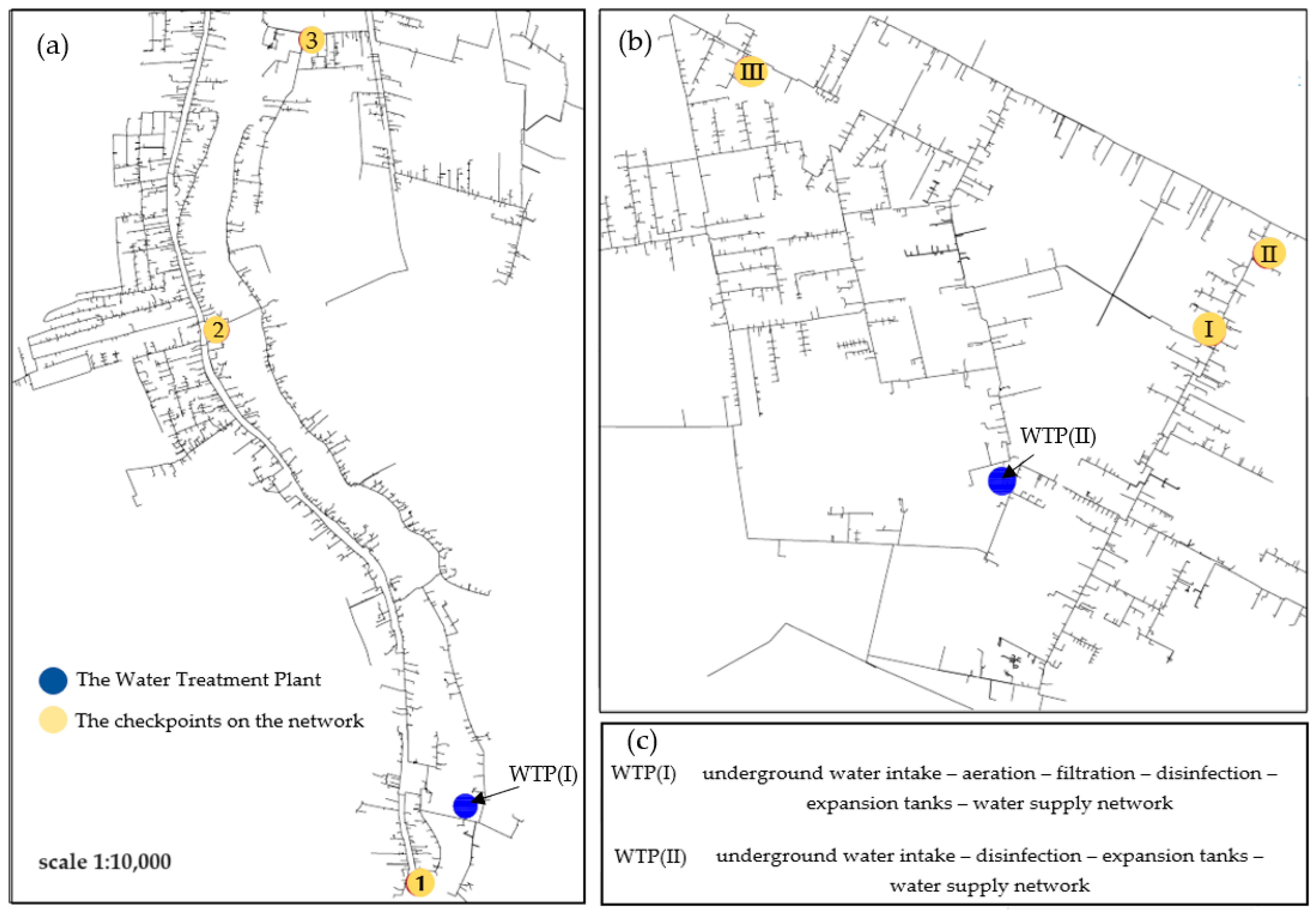
The research was carried out in two distribution systems that differed in the size of the supply area and the number of inhabitants supplied with tap water (detailed information about collective water supply systems is presented in Table 1). The research was carried out on water supply networks located in the south-eastern part of Poland (Lublin Voivodeship). For each distribution system (DS(I) and DS(II)), four control points were selected to assess the quality variation depending on the distance between the points and the water treatment plant (WTP). To have a clear picture of the water quality before it enters the distribution system, the outlet from the water treatment plant was selected as one of the sampling points. The water collected at WTP(I) is underground water rich in iron and manganese compounds, which is subjected to the following treatment processes, i.e., aeration, filtration, and disinfection. In turn, groundwater captured at WTP(II) is water that meets the guidelines for drinking water, which is directed directly to the network after the disinfection process. The detailed research area and sampling points are shown in Figure 1. The distances of the selected control points from the WTP (taking into account the shortest water transport route) were, respectively, for DS(I): P-1: 1 km, P-2: 4.1 km, and P-3: 6.2 km and for DS(II): P-I: 3.2 km, P-II: 3.7 km and P-III: 3.6 km. The selection of control points was mainly guided by the possibility of frequent collection of water samples for analysis, which is why public places, such as schools and administrative buildings, were selected.
2.2. Taking Samples for Analysis
Water samples were collected 2 days a week from eight control points for a period of 1 month (from 20 September to 20 October). Samples were taken from water intakes (WTP(I) and WTP(II)) and six consumer taps. Taking into account variable water consumption due to daily use, water was always collected on the same day at the same time. Water samples were collected in 1 L polyethylene terephthalate bottles (PET) and 0.5 L sterile glass bottles, which were then transported in an ice chest to the laboratory within 1 h.
2.3. Analysis of Physicochemical Water Quality
The quality of tap water was assessed using the methods presented in Table 2. The tests were carried out by applicable research procedures.
2.4. Water Stability Index
2.4.1. Biological Stability of Water
Biological stability was assessed based on the content of biogenic compounds: carbon, nitrogen, and phosphorus. The following threshold values determining the biological stability of water were adopted [22]: BDOC ≤ 0.25 mg C/L, ∑Ninorg. ≤ 0.2 mg N/L, P-PO43− ≤ 0.01 g PO43−/L.
Water can be considered biologically stable if at least two of the three given criteria are met. Based on the obtained test results, the percentage of samples that met the biological stability criteria was determined. Additionally, the bacteriological quality of water was assessed based on the content of Escherichia coli bacteria using membrane filtration on Endo WG ISO 9308-1 agar (BTL, Warszawa, Poland).
2.4.2. Physical Stability of Water
2.4.3. Chemical Stability of Water
Chemical stability was determined based on an indirect method for assessing the aggressiveness and corrosivity of water. The following indices were used in the research: Langelier (IL), Ryznar (IR), and Larson–Skold (ILS), the detailed method of determination of which is presented in Table 3.
3. Results and Discussion
The minimum, average, maximum, and standard deviation of the physicochemical parameters obtained for tap water collected at WTP(I) and WTP(II) and at various points of the distribution system are presented in Table 4 and Table 5.
The obtained test results conclude that the tested tap water samples met the requirements for water intended for human consumption. Only one sample taken from the P-1 control point for DS(I) exceeded the turbidity value (1.37 NTU). The recommended value of this parameter according to the guidelines should be acceptable to consumers and should not exceed 1.0 NTU. In the tested tap water collected from WTP(I) and WTP(II), the average turbidity was 0.68 NTU and 0.65 NTU, respectively. However, the average values obtained at the sampling points were, for DS(I), 0.82 NTU (P-1), 0.79 NTU (P-2), and 0.69 NTU (P-3), and for DS(II), 0.73 NTU (P-I), 0.74 NTU (P-II), and 0.68 NTU (P-III). Based on the obtained tests, it can be concluded that the water supplied to consumers was characterized by physical stability (for DS(I), 97% of water samples obtained values below 0.8 NTU, and for DS(II) 87.5% (Table 4)). Another important parameter that may affect the taste, smell, and color of drinking water is temperature. Table 4 shows that the temperature at WTP(I) and WTP(II) ranged from 10.10 to 11.80 °C, and at the intake points between 14.80 and 19.00 °C. The color of water in all analyzed samples was visually acceptable. The organoleptic parameters of water generally did not deteriorate during water transport from the treatment plant to other selected points. However, it should be assumed that this is not a complete picture of the water quality in these distribution systems, because the points in the internal installations concerned public buildings that are under constant supervision of the sanitary inspection; hence, the administrators of these facilities take care of their technical condition.
The average concentration of residual chlorine at the sampling points ranged from 0.06 to 0.09 mg/L (maximum normative value 0.3 mg/L). The low concentration of chlorine recorded did not affect the deterioration of the bacteriological quality of water—no Escherichia coli bacteria were detected in water samples [Table 4]. The decrease in the concentration of residual chlorine in the system may be related to organic sediments entering the water from pipes and as a result of contact with the biofilm formed on the internal surfaces of water pipes [25].
The captured groundwater obtained hardness values of 294 mg CaCO3/L (WTP(I)) and 360 mg CaCO3/L (WTP(II)), which indicates that they are extremely hard water. The presence of alkaline earth elements such as Ca (97.16–141.20 mg/L) and Mg (12.42–20.51 mg/L) contributes to the high hardness value in the examined area [Table 4 and Table 5]. The hardness of a groundwater sample is a practical value for determining the quality of water for domestic, agricultural, and industrial purposes. Soft water contains 0–60 mg CaCO3/L, medium-hard water contains 61–120 mg CaCO3/L, hard water contains 121–180 mg CaCO3/L, and extremely hard water contains > 181 mg CaCO3/L [26]. Although high levels of hardness are not harmful to health, both extremely soft (less than 60 mg CaCO3/L) and excessively hard water (more than 180 mg CaCO3/L) are considered undesirable [27]. A hardness of 200 mg CaCO3/L may cause minerals to accumulate on the fittings (especially during heating), and scale deposition may restrict water flow. In addition, this type of water is also characterized by poor foaming efficiency of soap and other detergents. Soft waters (<100 mg CaCO3/L), on the other hand, have a low buffering capacity and may be more corrosive to water pipes, causing the presence of heavy metals such as cadmium, copper, lead, and zinc in drinking water [28]. However, it should be remembered that hardness concentrations in the range of 60–500 mg CaCO3/L are within the limits of aesthetic acceptability for drinking water [6]. Calcium and alkalinity are known as pH stabilizers in water, but they must be maintained at a certain level to properly perform their roles [25].
Due to the influence of heavy metal ions on human metabolism, the analysis of their content is an important part of public health research [29,30]. International water quality regulations lower the maximum allowable levels of metals that are potentially toxic to humans. The average concentrations of all tested metals in the analyzed water samples did not exceed the normative values [6] and therefore did not pose any health risks to consumers. The range of chromium in water at WTP(I) was 0.17–0.92 µg/L, and in WTP(II) 0.27–1.22 µg/L [Table 5]. However, at the controlled points in the network, the average for DS(I) was 0.48 µg/L, and for DS(II) the value was 30% higher—0.68 µg/L (the permissible chromium concentration is 50 µg/L [6]). Significant differences were also observed in nickel concentrations in the analyzed groundwater. In WTP(I) water samples, Ni values ranged from 0.07 to 0.63 µg/L, and for WTP(II) from 1.52 to 6.31 µg/L (permissible value 20 µg/L [6]) [Table 5]. Ni occurs naturally in rocks and soil, from where it can be released into groundwater. Moreover, nickel may also be present in tap water as a result of corrosion or the abrasion of elements of pipeline systems made of materials containing this element, such as stainless steel or chrome–nickel. In the case of DS(I), at control points P-1 and P-2, a 63% and 39% increase in the content of this metal in tap water was recorded, which is due to the materials used to construct the internal installation. The average copper content also increased during water transport. In water samples taken from WTP(I) and WTP(II), Cu reached an average value of 4.59 µg/L and 6.85 µg/L, while higher values were recorded in the consumer’s tap (6.36 µg/L and 21.67 µg/L for DS(I) and DS(II)). However, Cu values were still well below the permitted limit of 2.0 mg/L [6]. Small amounts of copper are essential for good health, but too much of it can be very harmful. Consumption of large amounts of copper compounds may cause death due to failure of the nervous system, liver, and kidneys [31]. The next metal analyzed was lead—the average concentration of Pb in drinking water samples ranges from 0.19 to 2.44 µg/L (permissible value 10 µg/L). Lead is a poisonous metal that can damage nerve connections (especially in young children) and cause blood and brain disorders (damages the hematopoietic system) [32]. The content of cadmium, iron, and manganese also did not exceed the normative values and their values in tap water samples were 0–4.91 µg Cd/L, 0.01–0.09 mg Fe/L, and 1.35–11.82 µg Mn/L. The ranking order of average heavy metal concentrations in tap water detected in this study was, for WTP(I), Zn > Fe > Mn > Cu > Pb > Cr > Ni > Cd, and for WTP(II), Zn > Fe > Cu > Mn > Ni > Pb > Cr > Cd [Table 5]. It was found that the content of heavy metals during the transport of water from WTP(I) to other intake points increased in the case of Zn (from 0.05 to 0.12 mg/L), Ni (from 0.25 to 0.43 µm/L), Cu (from 4.59 to 6.36 µm/L), Cd (from 0.02 to 0.07 µm/L), and Pb (from 0.44 to 0.55 µm/L). In the case of WTP(II), the increase occurred for Fe (from 0.03 to 0.04 mg/L), Mn (from 1.74 to 1.82 µm/L), Ni (from 2.80 to 2.87 µm/L), Cu (from 6.86 to 21.67 µm/L), Cd (from 0.31 to 0.62 µm/L), and Pb (from 0.77 to 0.99 µm/L) [Table 5]. The observed differences in the content of heavy metals in tap water resulted from both the different quality of the intake water as well as the different materials used to build internal installations and the age and condition of the pipes. Monitoring water quality in distribution systems is important for proper management, but the low concentrations measured highlight the need for sensitive meters. The concentrations of Na, Mg, K, and Ca cations were also determined in the analyzed water samples. The concentrations of these elements ranged from 12.53 to 22.11 mg Na/L, 11.80 to 21.35 mg Mg/L, 3.87 to 4.40 mg K/L, and 97.16 to 141.20 mg Ca/L [Table 5].
Some metals are necessary in trace amounts for proper metabolism and good health. Heavy metals, although naturally occurring, can pose a threat to the environment when levels exceed recommended standards. There is growing concern about increasing trace metal concentrations in drinking water [33]. The main sources of heavy metals are food and water, as well as industrial activities and traffic. Although water sources may be contaminated, water purification technological processes should remove most of the heavy metals before introducing water into the system (these pollutants are relatively easy to adsorb or precipitate [34]). However, it should be emphasized that the type of material used in distribution systems and home installations influences the content of heavy metals in consumers’ tap water [35]. Pipelines used in the past were usually made of galvanized pipes, which, in addition to Fe, contained high contents of heavy metals such as Mn, Ni, and Cr. As a result of pipeline corrosion, large amounts of metallic elements were released, which changed the chemical composition of water during its transport [36,37]. Previous studies often reported deterioration in the quality of water transported through extensive distribution systems [38]. In the analyzed case, the distribution system is made mainly of thermoplastic materials, i.e., PE and PVC, which are characterized by high corrosion resistance and low surface porosity. Plastics can also contribute to the leaching of heavy metals, including lead, which may be present in PVC pipes as a stabilizer [39].
A water quality assessment showed that the analyzed tap water was characterized by a lack of biological stability due to the increased content of biogenic substances (mainly inorganic nitrogen, which in all samples obtained values above 0.2 mg Ninorg/L (Table 4 and Table 6)). The dominant form of nitrogen was nitrate nitrogen, which constituted on average 93% and 98% of total nitrogen in DS(I) and DS(II). The content of Ninorg in DS(II) ranged from 1.85 to 5.81 mg Ninorg/L and was on average 67% higher than for DS(I). A higher phosphate content was also found for DS(II) (by 68% on average), which resulted from the proximity of arable fields around the intake. Nitrates and phosphates are some of the widespread substances polluting groundwater, mainly from agricultural activities and improper waste disposal. In agricultural areas, the main sources are fertilizers and manure, while in built-up areas it is open sewers and septic tank leaks [40]. In the case of BDOC, higher values were recorded at WTPs than at the point of consumption by consumers [Table 6]. This phenomenon could be caused by the partial consumption of nutrients by microbiocenosis located on the internal surfaces of water pipes. For micro-organisms, a biofilm is a much better form of existence than the planktonic form, because the biofilm structure provides a safe environment for bacteria in which access to nutrients is much easier [41]. Biofilms are more likely to form in nutrient-poor systems because starving cells located on the surface can obtain a continuous supply of nutrients [42]. More than 95% of the biomass in DWDS is in the form of biofilm, and only 5% can be detected in the planktonic form [43]. Based on the obtained test results, it was also found that the percentage of samples meeting two of the three analyzed water biostability criteria established for N, C, and P was in the case of DS(I), 62.5% (P-1), 37.5% (P-2), and 25% (P-3), and for DS(II), 12.5% (P-I), 25% (P-II), and 0% (P-III). Groundwater collected at WTP(II) had a higher content of biogenic components, which was determined by the proximity of agricultural fields not far from the water intake zone. In turn, the presence of C, N, and P in the water distributed through the distribution system will promote the growth of micro-organisms and thus increase the risk of secondary water contamination.
Using the results of physicochemical measurements of the analyzed waters, basic water corrosivity indicators were calculated, which are presented in Table 7. The table shows that the indicator values are similar for all analyzed waters. The average values obtained for the Langelier Saturation Index range from −0.03 to 0.13, which suggests a slight tendency to precipitate calcium. The parameter that changes during water transport is primarily water temperature. In the WTP, the average temperature value is 10.7 °C, while in consumers, the temperature was over 1.5 times higher. Tap water transported with DS(II) was characterized by higher values of conductivity (by 26%), calcium (12%), and alkalinity (by 17%), which had a direct impact on higher values of the Langelier Index. Therefore, this water has a greater predisposition to the formation of deposits inside the installation. The average values obtained using RSI were 7.07–7.37 (WTP(I)) and 6.91–7.23 (WTP(II)), which allows the water to be classified as slightly corrosive. It should be noted that the values are close to the 6.2 < IR < 6.8 range, which corresponds to the chemical stability of water (neutral nature of water). Based on the LSI index, it can be concluded that water is slightly corrosive, and the chlorides and sulfates present in the water will probably not hinder the formation of a natural protective layer against corrosion (LSI < 0.2). It should be noted, however, that tap water transported with DS(II) had a higher content of chlorides (by 40%) and sulfates (by 45%). The LSI index differs from IR and IL because it is based on the corrosive effects of chloride, sulfate, and bicarbonate ions, without taking into account other physicochemical factors such as pH, temperature, total dissolved solids, alkalinity, and calcium. When assessing the corrosiveness of water, several indicators should always be analyzed, as a single indicator may lead to false conclusions. The need to use different indexes results from the fact that groundwater usually has a very diverse composition, and the indexes differ in the parameters used: pH, hardness, alkalinity, CO2, temperature, calcium, chloride, and sulfate concentration. Research by Maeng et al. [44] shows that the greatest influence on corrosion rates is pH > alkalinity > Ca > hardness > temperature > TDS. The average values for pH, alkalinity, and calcium hardness in the analyzed waters were 7.32, 272.38 mg CaCO3/L, and 277.057 mg CaCO3/L for DS(I). In the case of DS(II), these values were 7.26, 318.37 mg CaCO3/L, and 309.69 mg CaCO3/L. Heavy metals are also an important water parameter based on which the corrosive properties of water can be assessed. Metals such as copper, iron, or manganese may intensify the corrosion rate in aqueous environments [45,46,47]. High levels of nitrates in water can also increase the acidity of the water and therefore the degree of corrosion of distribution materials [45]. In the discussed case, the content of heavy metals in tap water met the guidelines for the quality of water intended for human consumption, and their content was at a low level in both analyzed distribution systems [Table 5].
4. Conclusions
Monitoring the quality of tap water in the distribution system and the ability to estimate the risk of losing its sanitary safety is an important aspect of managing the collective water supply system. Based on the obtained test results, it was found that in both analyzed distribution systems, the water supplied to consumers met the guidelines for water intended for human consumption. It can be considered that the risk of uncontrolled changes in water quality in DSs with an average water production of <10,000 m3/d and water pipeline length < 150 km is very low. The water introduced into the system differed in the place of water intake and water purification technology, which influenced the final water quality. DS(II) showed higher values of hardness (by 22%), conductivity (by 26%), calcium (by 12%), alkalinity (by 17%), nitrates (by 200%), and DOC (by 36%). Differences were also noted in the content of heavy metals for DS(I). The order was as follows: Zn > Fe > Mn > Cu > Pb > Cr > Ni > Cd, and for DS(II): Zn > Fe > Cu > Mn > Ni > Pb > Cr > Cd. It was found that the content of heavy metals during water transport from WTP(I) to other intake points increased in the case of Zn, Ni, Cu, Cd, and Pb. However, for WTP(II), an increase occurred for Fe, Mn, Ni, Cu, Cd, and Pb. The observed differences in the content of heavy metals in tap water resulted both from the different quality of the intake water as well as from different materials used to build internal installations and their age and technical condition. The analyzed tap waters were characterized by physical stability (for DS(I), 97% of samples obtained values below 0.8 NTU, and for DS(II), 87.5%) and chemical stability (the determined Langelier, Ryznar, and Larson–Skold Indexes indicate the slightly corrosive nature of water with a tendency to precipitate sediments). However, in both cases, the water did not meet the water biostability guidelines due to the increased content of biogenic substances. The presence of nutrients may pose a risk of secondary development of micro-organisms in the distribution system; however, no presence of Escherichia coli bacteria was detected at the controlled intake points. Ensuring and maintaining good water quality in the distribution system is a priority task for managers of water supply companies; hence, monitoring the quality of tap water is necessary for the proper management of these systems. The analyzed case concerned a small water supply network, while in the case of extensive networks, the possibility of uncontrolled changes in water quality is much greater.
Author Contributions
Conceptualization, A.D. and B.K.; methodology, A.D., B.K. and D.P.; formal analysis, A.D.; investigation, A.D., E.W. and I.K.; data curation, A.D., B.K. and D.P.; writing—original draft preparation, A.D.; writing—review and editing, B.K. and D.P.; visualization, A.D.; supervision, A.D., B.K. and D.P.; funding acquisition, A.D and B.K. All authors have read and agreed to the published version of the manuscript.
Funding
The research leading to these results has received funding from the commissioned task entitled “VIA CARPATIA Universities of Technology Network named after the President of the Republic of Poland Lech Kaczyński” under the special purpose grant from the Minister of Education and Science, contract no. MEiN/2022/DPI/2578, as part of the action “In the neighborhood—inter-university research internships and study visits”.
Data Availability Statement
Data is contained within the article.
Acknowledgments
We would like to thank the water supply company for their co-operation and for allowing us to collect samples for analysis.
Conflicts of Interest
The authors declare no conflicts of interest.
References
- Bichai, F.; Smeets, P.W.M.H. Using QMRA-Based Regulation as a Water Quality Management Tool in the Water Security Challenge: Experience from the Netherlands and Australia. Water Res. 2013, 47, 7315–7326. [Google Scholar] [CrossRef] [PubMed]
- Liu, Z.; Tao, S.; Sun, Z.; Chen, Y.; Xu, J. Determination of Heavy Metals and Health Risk Assessment in Tap Water from Wuhan, China, a City with Multiple Drinking Water Sources. Water 2023, 15, 3709. [Google Scholar] [CrossRef]
- Olatunde, K.; Kane Patton, S.; Cameron, L.; Stankus, T.; James Milaham, P. Factors Affecting the Quality of Drinking Water in the United States of America: A Ten-Year Systematic Review. AJWR 2022, 10, 24–34. [Google Scholar] [CrossRef]
- Perveen, S. Amar-Ul-Haque Drinking Water Quality Monitoring, Assessment and Management in Pakistan: A Review. Heliyon 2023, 9, e13872. [Google Scholar] [CrossRef] [PubMed]
- Price, J.I.; Heberling, M.T. The Effects of Source Water Quality on Drinking Water Treatment Costs: A Review and Synthesis of Empirical Literature. Ecol. Econ. 2018, 151, 195–209. [Google Scholar] [CrossRef] [PubMed]
- Council Directive 98/83/EC of 3 November 1998 on the Quality of Water Intended for Human Consumption. Available online: https://eur-lex.europa.eu/legal-content/EN/TXT/?uri=celex%3A31998L0083 (accessed on 15 February 2024).
- World Health Organization. A Global Overview of National Regulations and Standards for Drinking-Water Quality; World Health Organization: Geneva, Switzerland, 2021. [Google Scholar]
- Zhang, J.; Li, W.; Chen, J.; Wang, F.; Qi, W.; Li, Y. Impact of Disinfectant on Bacterial Antibiotic Resistance Transfer between Biofilm and Tap Water in a Simulated Distribution Network. Environ. Pollut. 2019, 246, 131–140. [Google Scholar] [CrossRef] [PubMed]
- Liu, G.; Zhang, Y.; Knibbe, W.-J.; Feng, C.; Liu, W.; Medema, G.; van der Meer, W. Potential Impacts of Changing Supply-Water Quality on Drinking Water Distribution: A Review. Water Res. 2017, 116, 135–148. [Google Scholar] [CrossRef] [PubMed]
- Chen, L.; Ling, F.; Bakker, G.; Liu, W.-T.; Medema, G.; Van Der Meer, W.; Liu, G. Assessing the Transition Effects in a Drinking Water Distribution System Caused by Changing Supply Water Quality: An Indirect Approach by Characterizing Suspended Solids. Water Res. 2020, 168, 115159. [Google Scholar] [CrossRef] [PubMed]
- Jachimowski, A. Factors affecting water quality in a water supply network. J. Ecol. Eng. 2017, 18, 110–117. [Google Scholar] [CrossRef] [PubMed]
- Świetlik, J.; Magnucka, M. Chemical and Microbiological Safety of Drinking Water in Distribution Networks Made of Plastic Pipes. WIREs Water 2023, 11, e1704. [Google Scholar] [CrossRef]
- Act of 7 June 2001 on collective water supply and collective sewage disposal. J. Laws 2001, 72, 747. (In Polish)
- Lee, D.; Calendo, G.; Kopec, K.; Henry, R.; Coutts, S.; McCarthy, D.; Murphy, H.M. The Impact of Pipe Material on the Diversity of Microbial Communities in Drinking Water Distribution Systems. Front. Microbiol. 2021, 12, 779016. [Google Scholar] [CrossRef]
- Learbuch, K.L.G.; Smidt, H.; van der Wielen, P.W.J.J. Influence of Pipe Materials on the Microbial Community in Unchlorinated Drinking Water and Biofilm. Water Res. 2021, 194, 116922. [Google Scholar] [CrossRef] [PubMed]
- Gonzalez, S.; Lopez-Roldan, R.; Cortina, J.-L. Presence of Metals in Drinking Water Distribution Networks Due to Pipe Material Leaching: A Review. Toxicol. Environ. Chem. 2013, 95, 870–889. [Google Scholar] [CrossRef]
- Rożej, A.; Cydzik-Kwiatkowska, A.; Kowalska, B.; Kowalski, D. Structure and Microbial Diversity of Biofilms on Different Pipe Materials of a Model Drinking Water Distribution Systems. World J. Microbiol. Biotechnol. 2015, 31, 37–47. [Google Scholar] [CrossRef]
- Besner, M.; Lavoie, J.; Morissette, C.; Payment, P.; Prévost, M. Effect of Water Main Repairs on Water Quality. J. AWWA 2008, 100, 95–109. [Google Scholar] [CrossRef]
- Gholizadeh, A.; Mokhtari, M.; Naimi, N.; Shiravand, B.; Ehrampoush, M.H.; Miri, M.; Ebrahimi, A. Assessment of Corrosion and Scaling Potential in Groundwater Resources; a Case Study of Yazd-Ardakan Plain, Iran. Groundw. Sustain. Dev. 2017, 5, 59–65. [Google Scholar] [CrossRef]
- García-Ávila, F.; Ramos-Fernández, L.; Zhindón-Arévalo, C. Estimation of Corrosive and Scaling Trend in Drinking Water Systems in the City of Azogues, Ecuador. Rev. Ambient. Agua 2018, 13, e2237. [Google Scholar] [CrossRef]
- Vreeburg, J.H.G.; Schippers, D.; Verberk, J.Q.J.C.; van Dijk, J.C. Impact of Particles on Sediment Accumulation in a Drinking Water Distribution System. Water Res. 2008, 42, 4233–4242. [Google Scholar] [CrossRef]
- Wolska, M. Removal of Nutrients in Water Purification Technology Intended for Human Consumption; Oficyna Wydawnicza Politechniki Wrocławskiej: Wroclaw, Poland, 2015. (In Polish) [Google Scholar]
- Pietrucha-Urbanik, K.; Tchórzewska-Cieślak, B.; Papciak, D.; Skrzypczak, I. Analysis of Chemical Stability of Tap Water in Terms of Required Level of Technological Safety. Arch. Environ. Prot. 2017, 43, 3–12. [Google Scholar] [CrossRef]
- Atekwana, E.; Atekwana, E.; Rowe, R.; Werkemajr, D.; Legall, F. The Relationship of Total Dissolved Solids Measurements to Bulk Electrical Conductivity in an Aquifer Contaminated with Hydrocarbon. J. Appl. Geophys. 2004, 56, 281–294. [Google Scholar] [CrossRef]
- Baloïtcha, G.M.P.; Mayabi, A.O.; Home, P.G. Evaluation of Water Quality and Potential Scaling of Corrosion in the Water Supply Using Water Quality and Stability Indices: A Case Study of Juja Water Distribution Network, Kenya. Heliyon 2022, 8, e09141. [Google Scholar] [CrossRef]
- Sengupta, P. Potential Health Impacts of Hard Water. Int. J. Prev. Med. 2013, 4, 866–875. [Google Scholar]
- Sappa, G.; Ergul, S.; Ferranti, F. Water Quality Assessment of Carbonate Aquifers in Southern Latium Region, Central Italy: A Case Study for Irrigation and Drinking Purposes. Appl. Water Sci. 2014, 4, 115–128. [Google Scholar] [CrossRef]
- Rubenowitz-Lundin, E.; Hiscock, K.M. Water Hardness and Health Effects. In Essentials of Medical Geology; Springer: Berlin/Heidelberg, Germany, 2012; pp. 337–350. [Google Scholar]
- Mitra, S.; Chakraborty, A.J.; Tareq, A.M.; Emran, T.B.; Nainu, F.; Khusro, A.; Idris, A.M.; Khandaker, M.U.; Osman, H.; Alhumaydhi, F.A. Impact of Heavy Metals on the Environment and Human Health: Novel Therapeutic Insights to Counter the Toxicity. J. King Saud Univ. Sci. 2022, 34, 101865. [Google Scholar] [CrossRef]
- Bafe Dilebo, W.; Desta Anchiso, M.; Tereke Kidane, T.; Eskezia Ayalew, M. Assessment of Selected Heavy Metals Concentration Level of Drinking Water in Gazer Town and Selected Kebele, South Ari District, Southern Ethiopia. Int. J. Anal. Chem. 2023, 2023, 1524850. [Google Scholar] [CrossRef]
- Mohod, C.V.; Dhote, J. Review of Heavy Metals in Drinking Water and Their Effect on Human Health. Int. J. Innov. Res. Sci. Eng. Technol. 2013, 2, 2992–2996. [Google Scholar]
- Ehi-Eromosele, C.O.; Okiei, W.O. Heavy Metal Assessment of Ground, Surface and Tap Water Samples in Lagos Metropolis Using Anodic Stripping Voltammetry. Resour. Environ. 2012, 2, 82–86. [Google Scholar]
- Zhang, P.; Yang, M.; Lan, J.; Huang, Y.; Zhang, J.; Huang, S.; Yang, Y.; Ru, J. Water Quality Degradation Due to Heavy Metal Contamination: Health Impacts and Eco-Friendly Approaches for Heavy Metal Remediation. Toxics 2023, 11, 828. [Google Scholar] [CrossRef]
- Chowdhury, S.; Mazumder, M.A.J.; Al-Attas, O.; Husain, T. Heavy Metals in Drinking Water: Occurrences, Implications, and Future Needs in Developing Countries. Sci. Total Environ. 2016, 569–570, 476–488. [Google Scholar] [CrossRef]
- Górski, J.; Siepak, M. Assessment of Metal Concentrations in Tap-Water–from Source to the Tap: A Case Study from Szczecin, Poland. Geologos 2014, 20, 25–33. [Google Scholar] [CrossRef]
- Chen, W.; Chen, J. Formation and Prevention of Pipe Scale in Water Supply Pipelines with Anti-Corrosion Lining. Water Supply 2022, 22, 4006–4014. [Google Scholar] [CrossRef]
- Sun, H.; Shi, B.; Yang, F.; Wang, D. Effects of Sulfate on Heavy Metal Release from Iron Corrosion Scales in Drinking Water Distribution System. Water Res. 2017, 114, 69–77. [Google Scholar] [CrossRef]
- Dinelli, E.; Lima, A.; Albanese, S.; Birke, M.; Cicchella, D.; Giaccio, L.; Valera, P.; De Vivo, B. Major and Trace Elements in Tap Water from Italy. J. Geochem. Explor. 2012, 112, 54–75. [Google Scholar] [CrossRef]
- Kowalska, B.; Kowalski, D.; Rożej, A. Organic Compounds Migrating from Plastic Pipes into Water. J. Water Supply Res. Technol. Aqua. 2011, 60, 137–146. [Google Scholar] [CrossRef]
- Verma, A.; Sharma, A.; Kumar, R.; Sharma, P. Nitrate Contamination in Groundwater and Associated Health Risk Assessment for Indo-Gangetic Plain, India. Groundw. Sustain. Dev. 2023, 23, 100978. [Google Scholar] [CrossRef]
- Erdei-Tombor, P.; Kiskó, G.; Taczman-Brückner, A. Biofilm Formation in Water Distribution Systems. Processes 2024, 12, 280. [Google Scholar] [CrossRef]
- Hammes, F.; Berney, M.; Wang, Y.; Vital, M.; Köster, O.; Egli, T. Flow-Cytometric Total Bacterial Cell Counts as a Descriptive Microbiological Parameter for Drinking Water Treatment Processes. Water Res. 2008, 42, 269–277. [Google Scholar] [CrossRef]
- Flemming, H.-C.; Percival, S.L.; Walker, J.T. Contamination Potential of Biofilms in Water Distribution Systems. Water Supply 2002, 2, 271–280. [Google Scholar] [CrossRef]
- Maeng, M.; Hyun, I.; Choi, S.; Dockko, S. Effects of Rainfall Characteristics on Corrosion Indices in Korean River Basins. Desalin. Water Treat. 2015, 54, 1233–1241. [Google Scholar] [CrossRef]
- Alvarez-Bastida, C.; Martínez-Miranda, V.; Vázquez-Mejía, G.; Solache-Ríos, M.; Fonseca-Montes De Oca, G.; Trujillo-Flores, E. The Corrosive Nature of Manganese in Drinking Water. Sci. Total Environ. 2013, 447, 10–16. [Google Scholar] [CrossRef]
- Bastidas, D.M.; Criado, M.; Fajardo, S.; La Iglesia, V.M.; Cano, E.; Bastidas, J.M. Copper Deterioration: Causes, Diagnosis and Risk Minimisation. Int. Mater. Rev. 2010, 55, 99–127. [Google Scholar] [CrossRef]
- Sarin, P.; Snoeyink, V.L.; Bebee, J.; Jim, K.K.; Beckett, M.A.; Kriven, W.M.; Clement, J.A. Iron Release from Corroded Iron Pipes in Drinking Water Distribution Systems: Effect of Dissolved Oxygen. Water Res. 2004, 38, 1259–1269. [Google Scholar] [CrossRef] [PubMed]
Figure 1.
Research area—location of checkpoints: (a) first distribution system—DS(I) with checkpoints 1, 2, 3; (b) second distribution system—DS(II) with checkpoints I, II, IIII, (c) description of water treatment technology for WTP(I) and WTP(II).
Figure 1.
Research area—location of checkpoints: (a) first distribution system—DS(I) with checkpoints 1, 2, 3; (b) second distribution system—DS(II) with checkpoints I, II, IIII, (c) description of water treatment technology for WTP(I) and WTP(II).


Table 1.
Information about collective water supply (data for 2023).
| Parameter | DS(I) | DS(II) |
|---|---|---|
| Average annual water production in m3/d | 819 | 695 |
| Estimated number of people supplied with water from the water supply system | 5642 | 3065 |
| Current status of the water supply network in km: | ||
| • With household connections | 143.50 | 75.28 |
| • Without connections | 82.64 | 38.94 |
| Type of construction material | PVC, PE | PVC, PE |
Table 2.
Method for assessing the physicochemical quality of tap water.
| Parameter | Unit | Method/Device |
|---|---|---|
| Temperature | °C | Digital HACCP thermometer (Hendi, Robakowo, Poland) |
| pH | - | Petameter Hach-Lange HQ 40d Multi (Hach-Lange, Düsseldorf, Germany) |
| Conductivity | µS/cm | |
| Turbidity | NTU | EUTECHTM TN-100 Turbidimeter (Thermo Scientific™, Gdańsk, Poland) |
| Color | mg Pt/L | Colorimetric method |
| Ammonium nitrogen | mg N-NH4+/L | Spectrophotometric method Hach-Lange DR 6000 spectrophotometer (Hach-Lange, Düsseldorf, Germany); (Spectrophotometric method: 8038; LCK341; 8039; LCK 348, 8051) |
| Nitrite nitrogen | mg N-NO2−/L | |
| Nitrate nitrogen | mg N-NO3−/L | |
| Phosphorus | mg P-PO43−/L | |
| Sulfates | mg SO4−/L | |
| Alkalinity | mg CaCO3/L | Titration method |
| Hardness | mg CaCO3/L | |
| Chlorides | mg Cl−/L | |
| Free/Total chlorine | mg Cl/L | Photometer PC MULTIDirect (Lovibond® Water Testing, Dortmund, Germany) |
| Dissolved organic carbon (DOC), Biodegradable dissolved organic carbon (BDOC) * | mg C/L | Total organic carbon analyzer TOC-L, (Shimadzu, Markham, ON, Canada) |
| Mn, Fe, Cu, Cd, Cr, Zn, Pb, Ca, Na, K, Mg | ppm/L; ppb/L | Agilent 8900 ICP-MS Triple Quad (Agilent, Santa Clara, CA, USA) |
Note: * It was assumed that the following relation describes the content of BDOC in groundwater: BDOC = 9% DOC [22].
| Equation | Water Feature |
|---|---|
| Langelier Saturation Index (IL) | |
| IL = pH-pHs pHs = (9.3 + A + B) − (C + D) Where: pH = pH measured in situ. pHs = pH at saturation pHs A = (log10 [TDS*] − 1)/10, B = –13.12 × log10 (°C + 273) + 34.55, C = log10 [Ca+2 mg/L as CaCo3] − 0.4, D = log10 [Alkalinity as CaCo3], TDS = Total Dissolved Solids, TDS = E × ke, E − conductivity [µS/cm], ke = 0.55–0.8, assumed: 0.64 | IL > 0; Water can dissolve calcium compounds and its corrosion properties are enhanced. −0.5 < IL < +0.5; Water is stable: it does not tend to precipitate or dissolve calcium carbonate, and the corrosion properties are weakened. IL < 0; Water can precipitate lime and its corrosion properties are weakened. |
| Ryznar Stability Index (IR) | |
| IR = 2 pHs-pH Where: pHs = pH at saturation pH = pH measured in situ. | IR < 5.5 Heavy scales likely to form 5.5 < IR < 6.2 Moderate scale-forming 6.2 < IR < 6.8 is considered neutral 6.8 < IR < 8.5 Low corrosion IR > 8.5 High corrosion |
| Larson Skold Index (ILS) | |
Cl−, SO42−, HCO3−—concentrations of chlorides, sulfates, and bicarbonates (total alkalinity of water) expressed in mval/L. | <0.8; chlorides and sulfates do not participate in the formation of natural layers protecting steel surfaces (they are not part of them and do not cause corrosion) 0.8 ÷ 1.2; chlorides and sulfates may participate in the formation of natural layers on steel surfaces and the corrosion rate may be increased >1.2; a significant rate of local corrosion is expected |
Table 4.
Summary of the results of the quality of tap water collected at the WTP and selected points of the distribution system.
Table 4.
Summary of the results of the quality of tap water collected at the WTP and selected points of the distribution system.
| DS(I) | |||||||||||||||||
| Parameter | Unit | WTP(I) | P-1 | P-2 | P-3 | ||||||||||||
| MIN | MAX | Mean | SD | MIN | MAX | Mean | SD | MIN | MAX | Mean | SD | MIN | MAX | Mean | SD | ||
| Temperature | °C | 10.10 | 11.80 | 10.72 | 0.63 | 17.00 | 18.90 | 17.68 | 0.70 | 16.80 | 18.50 | 17.60 | 0.60 | 15.90 | 18.00 | 17.08 | 0.69 |
| Ph | - | 7.29 | 7.35 | 7.31 | 0.02 | 7.30 | 7.40 | 7.33 | 0.04 | 7.30 | 7.40 | 7.33 | 0.03 | 7.29 | 7.33 | 7.31 | 0.01 |
| Conductivity | µS/cm | 481 | 525 | 481 | 12.93 | 491 | 522 | 506 | 11.61 | 481 | 533 | 508 | 17.55 | 475 | 535 | 502 | 19.15 |
| Turbidity | NTU | 0.52 | 0.82 | 0.68 | 0.10 | 0.57 | 1.37 | 0.82 | 0.24 | 0.60 | 0.97 | 0.79 | 0.14 | 0.64 | 0.82 | 0.69 | 0.06 |
| Ammonium nitrogen | mg N-NH4+/L | 0.02 | 0.22 | 0.10 | 0.06 | 0.00 | 0.16 | 0.03 | 0.05 | 0.00 | 0.13 | 0.03 | 0.04 | 0.00 | 0.09 | 0.03 | 0.03 |
| Nitrite nitrogen | mg N-NO2−/L | 0.01 | 0.02 | 0.01 | 0.00 | 0.01 | 0.02 | 0.01 | 0.00 | 0.00 | 0.09 | 0.02 | 0.03 | 0.01 | 0.02 | 0.01 | 0.00 |
| Nitrate nitrogen | mg N-NO3−/L | 0.40 | 2.40 | 0.84 | 0.66 | 0.60 | 2.40 | 1.13 | 0.75 | 0.70 | 2.20 | 1.31 | 0.71 | 0.70 | 2.70 | 1.35 | 0.79 |
| Phosphorus | mg P-PO43−/L | 0.00 | 0.05 | 0.02 | 0.02 | 0.00 | 0.04 | 0.01 | 0.01 | 0.00 | 0.04 | 0.01 | 0.01 | 0.00 | 0.06 | 0.03 | 0.02 |
| Alkalinity | mg CaCO3/L | 255 | 280 | 272 | 8.43 | 250 | 285 | 271 | 10.61 | 248 | 285 | 272 | 10.81 | 255 | 280 | 274 | 8.35 |
| Hardness | mg CaCO3/L | 275 | 303 | 294 | 9.82 | 280 | 298 | 293 | 5.94 | 280 | 308 | 297 | 8.43 | 278 | 313 | 299 | 11.18 |
| Chlorides | mg Cl−/L | 10.65 | 17.75 | 13.98 | 2.41 | 10.65 | 17.75 | 14.20 | 2.68 | 10.65 | 24.85 | 14.64 | 4.42 | 10.65 | 21.30 | 13.76 | 3.52 |
| Sulfates | mg SO42−/L | 34.00 | 39.00 | 37.17 | 1.72 | 34.00 | 39.00 | 36.50 | 1.76 | 36.00 | 38.00 | 37.00 | 0.89 | 35.00 | 37.00 | 36.17 | 0.75 |
| Free chlorine | mg Cl/L | 0.00 | 0.35 | 0.12 | 0.12 | 0.03 | 0.16 | 0.09 | 0.04 | 0.03 | 0.09 | 0.06 | 0.02 | 0.04 | 0.09 | 0.07 | 0.02 |
| Total chlorine | mg Cl/L | 0.05 | 0.31 | 0.17 | 0.10 | 0.15 | 0.26 | 0.19 | 0.04 | 0.17 | 0.22 | 0.20 | 0.02 | 0.13 | 0.27 | 0.18 | 0.06 |
| DOC | mg C/L | 0.56 | 23.85 | 12.53 | 9.38 | 0.13 | 3.30 | 0.93 | 1.05 | 0.04 | 4.29 | 1.58 | 1.58 | 0.48 | 5.97 | 1.87 | 1.99 |
| BDOC | mg C/L | 0.06 | 2.53 | 1.33 | 0.99 | 0.01 | 0.35 | 0.10 | 0.11 | 0.00 | 0.45 | 0.17 | 0.17 | 0.05 | 0.63 | 0.20 | 0.21 |
| Escherichia coli | CFU/100 mL | 0.00 | 0.00 | 0.00 | 0.00 | 0.00 | 0.00 | 0.00 | 0.00 | 0.00 | 0.00 | 0.00 | 0.00 | 0.00 | 0.00 | 0.00 | 0.00 |
| DS(II) | |||||||||||||||||
| Parameter | Unit | WTP(II) | P-I | P-II | P-III | ||||||||||||
| Temperature | °C | 10.10 | 11.80 | 10.78 | 0.73 | 14.80 | 17.70 | 15.88 | 0.99 | 15.60 | 19.00 | 17.97 | 1.23 | 16.40 | 18.90 | 17.42 | 1.11 |
| Ph | - | 7.19 | 7.30 | 7.23 | 0.03 | 7.21 | 7.29 | 7.24 | 0.03 | 7.23 | 7.35 | 7.27 | 0.05 | 7.27 | 7.33 | 7.29 | 0.02 |
| Conductivity | µS/cm | 609 | 653 | 609 | 18.23 | 618 | 669 | 639.5 | 21.33 | 606 | 669 | 637.3 | 24.63 | 621 | 675 | 644.9 | 23.28 |
| Turbidity | NTU | 0.58 | 0.75 | 0.65 | 0.07 | 0.55 | 0.96 | 0.73 | 0.14 | 0.62 | 0.94 | 0.74 | 0.11 | 0.55 | 0.82 | 0.68 | 0.10 |
| Ammonium nitrogen | mg N-NH4+/L | 0.00 | 0.08 | 0.04 | 0.03 | 0.00 | 0.15 | 0.07 | 0.05 | 0.00 | 0.05 | 0.02 | 0.02 | 0.00 | 0.08 | 0.03 | 0.03 |
| Nitrite nitrogen | mg N-NO2−/L | 0.00 | 0.01 | 0.01 | 0.00 | 0.01 | 0.03 | 0.02 | 0.01 | 0.00 | 0.04 | 0.01 | 0.01 | 0.01 | 0.02 | 0.01 | 0.00 |
| Nitrate nitrogen | mg N-NO3−/L | 2.30 | 4.70 | 3.53 | 0.89 | 2.10 | 4.64 | 3.41 | 0.98 | 2.20 | 5.80 | 3.48 | 1.37 | 1.80 | 4.86 | 3.55 | 1.20 |
| Phosphorus | mg P-PO43−/L | 0.00 | 0.07 | 0.03 | 0.03 | 0.00 | 0.17 | 0.07 | 0.05 | 0.00 | 0.11 | 0.05 | 0.04 | 0.00 | 0.10 | 0.07 | 0.03 |
| Alkalinity | mg CaCO3/L | 315 | 325 | 319 | 4.43 | 315 | 325 | 319 | 4.17 | 310 | 330 | 318 | 7.43 | 300 | 325 | 316 | 8.02 |
| Hardness | mg CaCO3/L | 343 | 373 | 360 | 10.04 | 238 | 375 | 348 | 45.27 | 353 | 380 | 367 | 8.96 | 365 | 375 | 369 | 3.45 |
| Chlorides | mg Cl−/L | 19.53 | 28.40 | 23.52 | 3.11 | 17.75 | 28.40 | 23.74 | 3.14 | 19.53 | 28.40 | 24.41 | 2.46 | 19.53 | 28.40 | 24.09 | 2.87 |
| Sulfates | mg SO42−/L | 50.00 | 54.00 | 51.67 | 1.37 | 48.00 | 55.00 | 52.00 | 2.45 | 50.00 | 53.00 | 51.50 | 1.05 | 51.00 | 54.00 | 52.40 | 1.14 |
| Free chlorine | mg Cl/L | 0.04 | 0.09 | 0.07 | 0.02 | 0.00 | 0.23 | 0.07 | 0.08 | 0.03 | 0.11 | 0.06 | 0.03 | 0.00 | 0.09 | 0.04 | 0.03 |
| Total chlorine | mg Cl/L | 0.17 | 0.29 | 0.22 | 0.04 | 0.09 | 0.24 | 0.18 | 0.04 | 0.14 | 0.20 | 0.17 | 0.02 | 0.00 | 0.21 | 0.11 | 0.08 |
| DOC | mg C/L | 0.37 | 21.89 | 15.71 | 8.74 | 0.35 | 6.64 | 2.17 | 2.01 | 0.11 | 9.20 | 3.18 | 2.89 | 0.01 | 12.61 | 3.01 | 4.53 |
| BDOC | mg C/L | 0.04 | 2.32 | 1.66 | 0.93 | 0.04 | 0.70 | 0.23 | 0.21 | 0.01 | 0.97 | 0.23 | 0.31 | 0.00 | 1.35 | 0.31 | 0.48 |
| Escherichia coli | CFU/100 mL | 0.00 | 0.00 | 0.00 | 0.00 | 0.00 | 0.00 | 0.00 | 0.00 | 0.00 | 0.00 | 0.00 | 0.00 | 0.00 | 0.00 | 0.00 | 0.00 |
Table 5.
The concentration of metals in water directed to the network and in selected points of the distribution system.
Table 5.
The concentration of metals in water directed to the network and in selected points of the distribution system.
| Metal | Unit | DS(I) | |||||||||||||||
| WTP(I) | P-1 | P-2 | P-3 | ||||||||||||||
| Min | Max | Mean | SD | Min | Max | Mean | SD | Min | Min | Mean | SD | Min | Max | Mean | SD | ||
| Na | ppm/L | 12.95 | 17.34 | 16.19 | 1.23 | 12.53 | 17.34 | 16.19 | 1.54 | 13.24 | 17.14 | 16.08 | 1.23 | 13.74 | 18.80 | 16.43 | 1.38 |
| Mg | ppm/L | 12.42 | 16.50 | 14.69 | 1.28 | 11.80 | 15.87 | 14.83 | 1.31 | 12.31 | 16.06 | 14.83 | 1.16 | 12.79 | 15.98 | 14.95 | 0.97 |
| K | ppm/L | 3.62 | 4.21 | 3.89 | 0.20 | 3.56 | 4.08 | 3.92 | 0.17 | 3.63 | 4.07 | 3.87 | 0.16 | 3.75 | 4.11 | 3.92 | 0.10 |
| Ca | ppm/L | 97.16 | 141.20 | 111.83 | 13.59 | 104.00 | 133.38 | 112.20 | 9.17 | 99.02 | 112.55 | 107.69 | 4.51 | 106.96 | 131.43 | 112.05 | 7.99 |
| Zn | ppm/L | 0.02 | 0.10 | 0.05 | 0.03 | 0.04 | 0.12 | 0.06 | 0.03 | 0.04 | 0.09 | 0.05 | 0.02 | 0.05 | 0.52 | 0.26 | 0.18 |
| Fe | ppm/L | 0.03 | 0.07 | 0.05 | 0.02 | 0.03 | 0.08 | 0.05 | 0.02 | 0.01 | 0.13 | 0.05 | 0.03 | 0.02 | 0.08 | 0.04 | 0.02 |
| Mn | ppb/L | 7.17 | 11.82 | 8.78 | 1.56 | 4.85 | 11.24 | 6.02 | 2.13 | 5.85 | 9.80 | 7.29 | 1.33 | 5.23 | 11.08 | 6.55 | 1.93 |
| Cr | ppb/L | 0.17 | 0.92 | 0.48 | 0.23 | 0.12 | 1.02 | 0.51 | 0.30 | 0.26 | 1.25 | 0.55 | 0.34 | 0.11 | 0.66 | 0.39 | 0.19 |
| Ni | ppb/L | 0.07 | 0.63 | 0.25 | 0.20 | 0.30 | 1.75 | 0.68 | 0.50 | 0.07 | 1.81 | 0.41 | 0.58 | 0.10 | 0.33 | 0.22 | 0.09 |
| Cu | ppb/L | 2.98 | 14.62 | 4.59 | 3.84 | 3.88 | 6.81 | 5.42 | 1.04 | 1.64 | 19.10 | 4.76 | 5.82 | 4.51 | 18.24 | 8.91 | 5.88 |
| Cd | ppb/L | 0.00 | 0.11 | 0.02 | 0.04 | 0.00 | 0.02 | 0.01 | 0.01 | 0.00 | 1.12 | 0.16 | 0.39 | 0.00 | 0.30 | 0.05 | 0.10 |
| Pb | ppb/L | 0.25 | 0.70 | 0.44 | 0.10 | 0.36 | 0.65 | 0.48 | 0.10 | 0.19 | 0.89 | 0.40 | 0.24 | 0.35 | 1.80 | 0.77 | 0.52 |
| Metal | Unit | DS(II) | |||||||||||||||
| WTP(II) | P-I | P-II | P-III | ||||||||||||||
| 17.91 | 21.44 | 20.33 | 1.17 | 21.13 | 22.11 | 21.61 | 0.37 | 19.19 | 21.55 | 20.55 | 0.90 | 19.44 | 21.55 | 20.32 | 0.85 | ||
| Mg | ppm/L | 18.44 | 20.51 | 19.90 | 0.68 | 19.96 | 21.35 | 20.60 | 0.48 | 18.47 | 20.74 | 19.68 | 0.79 | 18.60 | 20.98 | 19.66 | 0.83 |
| K | ppm/L | 3.97 | 4.30 | 4.22 | 0.12 | 4.14 | 4.44 | 4.31 | 0.10 | 3.87 | 4.40 | 4.20 | 0.16 | 3.88 | 4.31 | 4.18 | 0.16 |
| Ca | ppm/L | 119.50 | 128.37 | 124.52 | 2.71 | 119.77 | 134.01 | 125.78 | 4.67 | 111.98 | 128.53 | 122.84 | 5.27 | 114.46 | 127.36 | 122.90 | 4.55 |
| Zn | ppm/L | 0.01 | 0.33 | 0.09 | 0.11 | 0.02 | 0.12 | 0.06 | 0.04 | 0.01 | 0.08 | 0.04 | 0.02 | 0.03 | 0.23 | 0.10 | 0.07 |
| Fe | ppm/L | 0.02 | 0.09 | 0.03 | 0.03 | 0.03 | 0.09 | 0.04 | 0.03 | 0.01 | 0.09 | 0.04 | 0.03 | 0.01 | 0.08 | 0.04 | 0.02 |
| Mn | ppb/L | 1.43 | 2.43 | 1.74 | 0.34 | 1.71 | 2.16 | 1.84 | 0.17 | 1.35 | 2.25 | 1.76 | 0.30 | 1.55 | 2.49 | 1.85 | 0.33 |
| Cr | ppb/L | 0.27 | 1.22 | 0.69 | 0.32 | 0.24 | 0.81 | 0.60 | 0.21 | 0.54 | 1.26 | 0.77 | 0.25 | 0.25 | 1.08 | 0.67 | 0.29 |
| Ni | ppb/L | 1.52 | 6.31 | 2.80 | 1.64 | 2.19 | 4.02 | 2.85 | 0.70 | 1.63 | 4.80 | 2.92 | 1.11 | 1.61 | 5.43 | 2.85 | 1.60 |
| Cu | ppb/L | 1.56 | 17.55 | 6.86 | 6.60 | 3.09 | 12.00 | 5.21 | 3.40 | 3.28 | 86.18 | 22.68 | 29.55 | 20.11 | 92.68 | 37.11 | 27.96 |
| Cd | ppb/L | 0.02 | 1.87 | 0.31 | 0.69 | 0.01 | 4.91 | 0.86 | 1.98 | 0.02 | 0.29 | 0.10 | 0.12 | 0.01 | 0.30 | 0.09 | 0.11 |
| Pb | ppb/L | 0.19 | 2.44 | 0.77 | 0.76 | 0.34 | 1.45 | 0.77 | 0.41 | 0.27 | 1.57 | 0.84 | 0.47 | 0.83 | 1.77 | 1.38 | 0.32 |
Table 6.
Content of nutrients in the analyzed waters.
| N | BDOC | P | ||||||||||
|---|---|---|---|---|---|---|---|---|---|---|---|---|
| Min | Max | Mean | Number of Samples < 0.2 mg Ninorg/L [%] | Min | Max | Mean | Number of Samples < 0.25 mg C/L [%] | Min | Max | Mean | Number of Samples < 0.01 mg P-PO43−/L [%] | |
| DS(I) | ||||||||||||
| WTP(I) | 0.56 | 2.53 | 0.96 | 0 | 0.06 | 2.53 | 1.33 | 25 | 0.00 | 0.05 | 0.02 | 50 |
| P-1 | 0.61 | 2.42 | 1.18 | 0 | 0.01 | 0.35 | 0.10 | 87.5 | 0.00 | 0.04 | 0.01 | 62.5 |
| P-2 | 0.74 | 2.25 | 1.18 | 0 | 0.00 | 0.45 | 0.17 | 75 | 0.00 | 0.04 | 0.01 | 62.5 |
| P-3 | 0.76 | 2.73 | 1.39 | 0 | 0.05 | 0.63 | 0.20 | 75 | 0.00 | 0.06 | 0.03 | 37.5 |
| DS(II) | ||||||||||||
| WTP(II) | 2.3 | 4.73 | 3.58 | 0 | 0.36 | 2.28 | 1.66 | 0 | 0.00 | 0.07 | 0.03 | 37.5 |
| P-I | 2.27 | 4.52 | 3.50 | 0 | 0.05 | 0.70 | 0.23 | 62.5 | 0.00 | 0.17 | 0.07 | 12.5 |
| P-II | 2.26 | 5.81 | 3.50 | 0 | 0.01 | 0.97 | 0.23 | 87.5 | 0.00 | 0.11 | 0.05 | 12.5 |
| P-III | 1.85 | 4.88 | 3.59 | 0 | 0.00 | 1.35 | 0.32 | 71.4 | 0.00 | 0.10 | 0.07 | 14.3 |
Table 7.
Summary of calculated water corrosion indices.
| Langelier Index | Ryznar Index | Larson–Skold Index | |||||||
|---|---|---|---|---|---|---|---|---|---|
| Min | Max | Mean | Min | Max | Mean | Min | Max | Mean | |
| DS(I) | |||||||||
| WTP(I) | −0.09 | 0.09 | −0.03 | 7.12 | 7.50 | 7.37 | 0.12 | 0.16 | 0.14 |
| P-1 | 0.07 | 0.18 | 0.13 | 6.93 | 7.18 | 7.07 | 0.13 | 0.16 | 0.14 |
| P-2 | 0.04 | 0.20 | 0.11 | 7.00 | 7.22 | 7.11 | 0.12 | 0.20 | 0.15 |
| P-3 | 0.07 | 0.16 | 0.10 | 6.97 | 7.18 | 7.18 | 0.12 | 0.18 | 0.14 |
| DS(II) | |||||||||
| WTP(II) | −0.04 | 0.04 | 0.00 | 7.18 | 7.27 | 7.23 | 0.16 | 0.20 | 0.18 |
| P-I | 0.07 | 0.14 | 0.10 | 6.99 | 7.07 | 7.03 | 0.17 | 0.21 | 0.19 |
| P-II | 0.12 | 0.26 | 0.18 | 6.83 | 6.99 | 6.92 | 0.17 | 0.21 | 0.19 |
| P-III | 0.17 | 0.24 | 0.19 | 6.84 | 6.94 | 6.91 | 0.18 | 0.21 | 0.19 |
Disclaimer/Publisher’s Note: The statements, opinions and data contained in all publications are solely those of the individual author(s) and contributor(s) and not of MDPI and/or the editor(s). MDPI and/or the editor(s) disclaim responsibility for any injury to people or property resulting from any ideas, methods, instructions or products referred to in the content. |
© 2024 by the authors. Licensee MDPI, Basel, Switzerland. This article is an open access article distributed under the terms and conditions of the Creative Commons Attribution (CC BY) license (https://creativecommons.org/licenses/by/4.0/).
Share and Cite
MDPI and ACS Style
Domoń, A.; Kowalska, B.; Papciak, D.; Wojtaś, E.; Kamińska, I. Safety of Tap Water in Terms of Changes in Physical, Chemical, and Biological Stability. Water 2024, 16, 1221. https://doi.org/10.3390/w16091221
AMA Style
Domoń A, Kowalska B, Papciak D, Wojtaś E, Kamińska I. Safety of Tap Water in Terms of Changes in Physical, Chemical, and Biological Stability. Water. 2024; 16(9):1221. https://doi.org/10.3390/w16091221
Chicago/Turabian StyleDomoń, Andżelika, Beata Kowalska, Dorota Papciak, Edyta Wojtaś, and Iwona Kamińska. 2024. "Safety of Tap Water in Terms of Changes in Physical, Chemical, and Biological Stability" Water 16, no. 9: 1221. https://doi.org/10.3390/w16091221
Note that from the first issue of 2016, this journal uses article numbers instead of page numbers. See further details here.