
Inspection Method of Rope Arrangement in the Ultra-Deep Mine Hoist Based on Optical Projection and Machine Vision


Abstract
:1. Introduction
- The target is extremely similar to the background;
- The wider the scroll, the larger the scroll deformation in the projection image;
- The detection speed and robustness should meet the requirements of high speed.
2. How to Get the Required Projection
2.1. Projection Model of the Drum’s Rope Arrangement
2.1.1. Projection of the Single Coil Wire Rope
2.1.2. Projection of Multi Coil Wire Ropes
2.2. Determine the Installation Position of Point Light Source
3. Boundary Extraction and Feature Extraction of Rope Arrangement Projection
- There is a big difference between the shadow area and the illumination area;
- The gray value of shadow area in the image is stable and average, and there is no light noise;
- The upper limit of the gray value of the illumination area of the light source in the image is affected by the change of the light intensity of the external environment, and the lower limit is affected by the light intensity of the point light source here;
- Due to the influence of dust and oil on the wire rope, the project of the wire rope may be irregular and the gap between each other becomes unclear;
- Due to the influence of dust and oil on the background plate, there may be discrete dark spots in the light source area of the image (as shown in Figure 6c).
3.1. Boundary Extraction
3.2. Feature Extraction
4. Unsupervised Clustering
4.1. DBSCAN
- Until all points in Z have been visited; do
- (1)
- Pick a point that has not been visited;
- (2)
- Mark as a visited point;
- (3)
- If is a core point; then:
- (1)
- Find the set C of all points that are density reachable from .
- (2)
- C now forms a cluster. Mark all points within that cluster as being visited.
- Return the cluster assignments , …, with k the number of clusters. Points that have not been assigned to a cluster are considered noise or outliers.
4.2. Automatic Optimization of DBSCAN Distance Setting
5. Application Effect
5.1. Application Effect in the Laboratory
5.2. Application Effect in the Ultra-Deep Well Simulation Test Bench
6. Discussion and Conclusions
- For the different widths of the drum, this method can always detect the rope arrangement state stably and at high speed;
- If the ROI area width of the projection image exceeds 50 pixels, the subsequent correct detection can be ensured;
- The detection speed is related to the image size. When the image width is set to 70 pixels, the detection speed of the reel with 14 turns exceeds 300 fps. However, when the image width is set to 50 pixels, the detection speed of the reel with 95 turns exceeds 200 fps;
- The detection sensitivity of this method is higher than that of human eye observation, and it can detect the rope arranging fault earlier.
- This study reduces the dimension of the difficulties of the detection of rope arrangement by projection;
- This study replaces the problem of inevitable image distortion and overlap distortion in wide-roll shooting with the installation space requirement of the light source, which can be easily solved;
- This study can judge the rope arrangement fault using a single frame instead of the comparison of at least two frames, which has lower robustness during high-speed detection;
- The proposed adaptive Gaussian filtering method ensures the correct extraction of eigenvalues, and the designed distance thresholds of the DBSCAN method enables it to classify eigenvalues earlier and more accurately;
- It can be adapted to the detection of wide reels in ultra-deep mines; the detection speed of the reel with 95 turns can exceed 200 fps.
7. Patents
Author Contributions
Funding
Institutional Review Board Statement
Informed Consent Statement
Data Availability Statement
Conflicts of Interest
References
- Peng, X. Mechanism of the Multi-Layer Winding Drum and the Theory on Crossover Design in Deep Mine Hoisting. Ph.D. Thesis, College of Mechanical Engineering of Chongqing University, Chongqing, China, 2018. [Google Scholar]
- Peng, X.; Gong, X.S.; Liu, J.J. The study on crossover layouts of multi-layer winding grooves in deep mine hoists based on transverse vibration characteristics of catenary rope. Proc. Inst. Mech. Eng. 2019, 233, 118–132. [Google Scholar] [CrossRef]
- Santos, C.A.; Costa, C.O.; Batista, J. A vision-based system for measuring the displacements of large structures: Simultaneous adaptive calibration and full motion estimation. Mech. Syst. Signal Pr. 2016, 72–73, 678–694. [Google Scholar] [CrossRef]
- Xu, Y.; Brownjohn, J.M.W. Review of machine-vision based methodologies for displacement measurement in civil structures. J. Civ. Struct. Health Monit. 2017, 8, 91–110. [Google Scholar] [CrossRef] [Green Version]
- Zhao, J.; Bao, Y.; Guan, Z.; Zuo, W.; Li, J.; Li, H. Video-based multiscale identification approach for tower vibration of a cable-stayed bridge model under earthquake ground motions. Struct. Control Health Monit. 2019, 26, e2314. [Google Scholar] [CrossRef]
- Brownjohn, J.M.W.; Xu, Y.; Hester, D. Vision-Based Bridge Deformation Monitoring. Front. Built Environ. 2017, 3, 23. [Google Scholar] [CrossRef] [Green Version]
- Abolhasannejad, V.; Huang, X.; Namazi, N. Developing an Optical Image-Based Method for Bridge Deformation Measurement Considering Camera Motion. Sensors 2018, 18, 2754. [Google Scholar] [CrossRef] [PubMed] [Green Version]
- Shao, S.; Zhou, Z.; Deng, G.; Du, P.; Jian, C.; Yu, Z. Experiment of Structural Geometric Morphology Monitoring for Bridges Using Holographic Visual Sensor. Sensors 2020, 20, 1187. [Google Scholar] [CrossRef] [Green Version]
- Chen, C.; Chen, C.; Wu, W.; Tseng, H. Modal Frequency Identification of Stay Cables with Ambient Vibration Measurements Based on Nontarget Image Processing Techniques. Adv. Struct. Eng. 2012, 15, 929–942. [Google Scholar] [CrossRef]
- Winkler, J.; Fischer, G.; Christos, C.T. Measurement of Local Deformations in Steel Monostrands Using Digital Image Correlation. J. Bridge Eng. 2014, 19, 04014042. [Google Scholar] [CrossRef]
- Yao, J.; Xiao, X.; Chang, H. Video-based measurement for transverse vibrations of moving catenaries in mine hoist using mean shift tracking. Adv. Mech. Eng. 2015, 7, 168781401560807. [Google Scholar] [CrossRef] [Green Version]
- Yao, J.; Xiao, X.; Peng, A.; Jiang, Y.; Ma, C. Assessment of safety for axial fluctuations of head sheaves in mine hoist based on coupled dynamic model. Eng. Fail Anal. 2015, 51, 98–107. [Google Scholar] [CrossRef]
- Yao, J.; Xiao, X.; Liu, Y. Camera-based measurement for transverse vibrations of moving catenaries in mine hoists using digital image processing techniques. Meas. Sci. Technol. 2016, 27, 35003. [Google Scholar] [CrossRef]
- Wu, G.; Xiao, X.; Yao, J.; Song, C. Machine vision-based measurement approach for transverse vibrations of moving hoisting vertical ropes in mine hoists using edge location. Meas. Control 2019, 52, 554–566. [Google Scholar] [CrossRef]
- Wu, Z.; Tan, J.; Wang, Q.; Hu, Y. Research of Image Recognition Method for Visual Monitoring of Rope-arranging Fault of Hoist. Instrum. Technol. Sens. 2016, 10, 73–75. [Google Scholar]
- Xue, S.; Tan, J.; Wu, Z.; Wang, Q. In Vision-based Rope-arranging Fault Detection Method for Hoisting systems. In Proceedings of the 2018 IEEE International Conference on Information and Automation (ICIA), Wuyishan, China, 11–13 August 2018. [Google Scholar]
- Henriques, J.F.; Caseiro, R.; Martins, P.; Batista, J. High-Speed Tracking with Kernelized Correlation Filters. IEEE T Pattern Anal. 2015, 37, 583–596. [Google Scholar] [CrossRef] [Green Version]
- Bertinetto, L.; Valmadre, J.; Golodetz, S.; Miksik, O.; Torr, P.H. Staple: Complementary Learners for Real-Time Tracking. In Proceedings of the IEEE Conference on Computer Vision and Pattern Recognition (CVPR), Las Vegas, NV, USA, 26 June–1 July 2016. [Google Scholar]
- Schowengerdt, R.A. Remote Sensing. Models and Methods for Image Processing; Academic Press: Chestnut Hill, MA, USA, 1997; p. 521. [Google Scholar]
- Amoako-Yirenkyi, P.; Appati, J.K.; Dontwi, I.K. Performance Analysis of Image Smoothing Techniques on a New Fractional Convolution Mask for Image Edge Detection. Open J. Appl. Sci. 2016, 6, 478–488. [Google Scholar] [CrossRef] [Green Version]
- Duda, R.O.; Hart, P.E. Pattern Classification and Scene Analysis; Wiley: New York, NY, USA, 1973. [Google Scholar]
- Lipkin, B.S.; Rosenfeld, A. Picture Processing and Psychopictorics. Trans. Am. Microsc. Soc. 1972, 91, 2. [Google Scholar]
- Ding, L.; Goshtasby, A. On the Canny edge detector. Pattern Recogn. 2001, 34, 721–725. [Google Scholar] [CrossRef]
- Canny, J. A Computational Approach to Edge Detection. IEEE Trans. Pattern Anal. Mach. 1986, 8, 679–698. [Google Scholar] [CrossRef]
- Qiao, W.; Yang, Z.; Kang, Z.; Pan, Z. Short-term natural gas consumption prediction based on Volterra adaptive filter and improved whale optimization algorithm. Eng. Appl. Artif. Intel. 2020, 87, 103323. [Google Scholar] [CrossRef]
- Pedregosa, F. Scikit-learn: Machine Learning in Python. J. Mach. Learn. Res. 2011, 12, 2825–2830. [Google Scholar]
- Luxburg, U. A tutorial on spectral clustering. Stat. Comput. 2007, 17, 395–416. [Google Scholar] [CrossRef]
- Ester, M.; Kriegel, H.-P.; Sander, J.; Xu, X. A Density-Based Algorithm for Discovering Clusters in Large Spatial Databases with Noise. In Proceedings of the 2nd International Conference on Knowledge Discovery and Data Mining (KDD-96), Portland, OR, USA, 2–4 August 1996; pp. 226–231. [Google Scholar]
- Ankerst, M.; Breunig, M.M.; Kriegel, H.P.; Sander, J. OPTICS: Ordering Points to Identify the Clustering Structure. In Proceedings of the ACM SIGMOD International Conference on Management of Data, Philadelphia, PA, USA, 1–3 June 1999. [Google Scholar]
- Chen, J.; Salim, M.B.; Matsumoto, M. A Gaussian Mixture Model-Based Continuous Boundary Detection for 3D Sensor Networks. Sensors 2010, 10, 7632–7650. [Google Scholar] [CrossRef]
- Rodriguez, A.; Laio, A. Clustering by fast search and find of density peaks. Science 2014, 344, 1492–1496. [Google Scholar] [CrossRef] [Green Version]
- Mehta, P.; Bukov, M.; Wang, C.; Day, A.G.R.; Richardson, C.; Fisher, C.K.; Schwab, D.J. A high-bias, low-variance introduction to Machine Learning for physicists. Phys. Rep. 2019, 810, 1–124. [Google Scholar] [CrossRef]


| Methods | Timeliness | Implementation Difficulty and Cost | Accuracy of Detection | Efficiency of Detection | Robustness |
|---|---|---|---|---|---|
| Manual inspections or manual guards | Low (the fault has occurred) | High | Moderate | Very slow | High |
| Image segmentation [15] | Low (the fault has occurred) | Low | 80–90% | 100 fps | Low |
| Template matching [16] | High (happening, at least two frames) | Low | 85–90% | 30–50 fps | Low |
| Video tracking (KCF [17]) | High (happening, at least two frames) | Low | 85–90% | 150–200 fps | Low |
| Video tracking (Staple [18]) | High (happening, at least two frames) | Low | 90–95% | 40–60 fps | Moderate |
| ours | High (happening, just one frame) | Low | >95% | 150–300 fps | High |
| Symbols and Abbreviations | Meaning | Symbols and Abbreviations | Meaning | Symbols and Abbreviations | Meaning |
|---|---|---|---|---|---|
| DBSCAN | Density-based spatial clustering of applications with noise | sum() | A function to calculate the sum | dy | The height difference of the projection intersection point and the highest projection point |
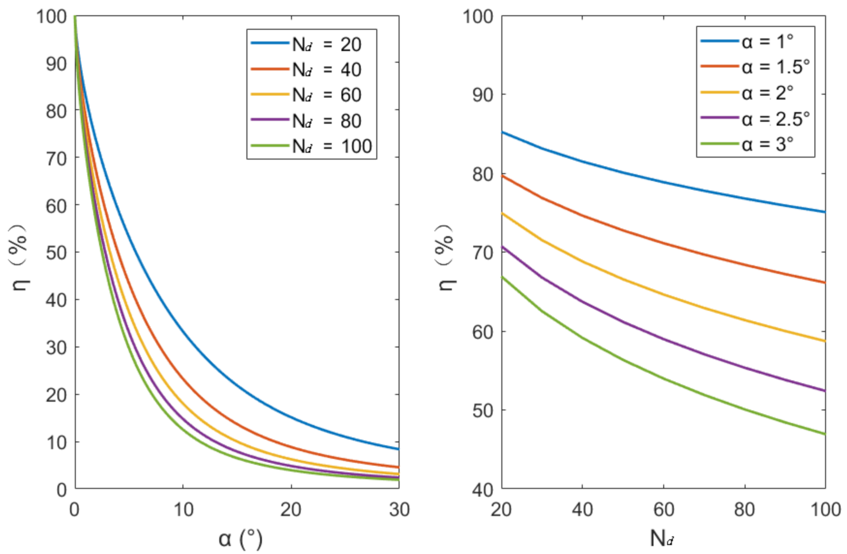
| KCFs | Kernelized correlation filters | min() | Calculate minimum | η | The ratio between dy and r |
| ROI | The area of interest | find(equation) | A function to find elements match the requirement | Nd | The ratio between R and r |
| OPTICS | Ordering points to identify the clustering structure | (x,y), (x1,y1) (x2,y2), (xt,yt) | Coordinate points | Lg | The width of the drum |
| G(x) | Gaussian filtering function | R | The radius of the central circle of the torus or the drum | Ng | The ratio between and 2r |
| dist() | A function to calculate the distance | r | The radius of the section circle of torus or the radius of the rope | The installation height of the point light source | |
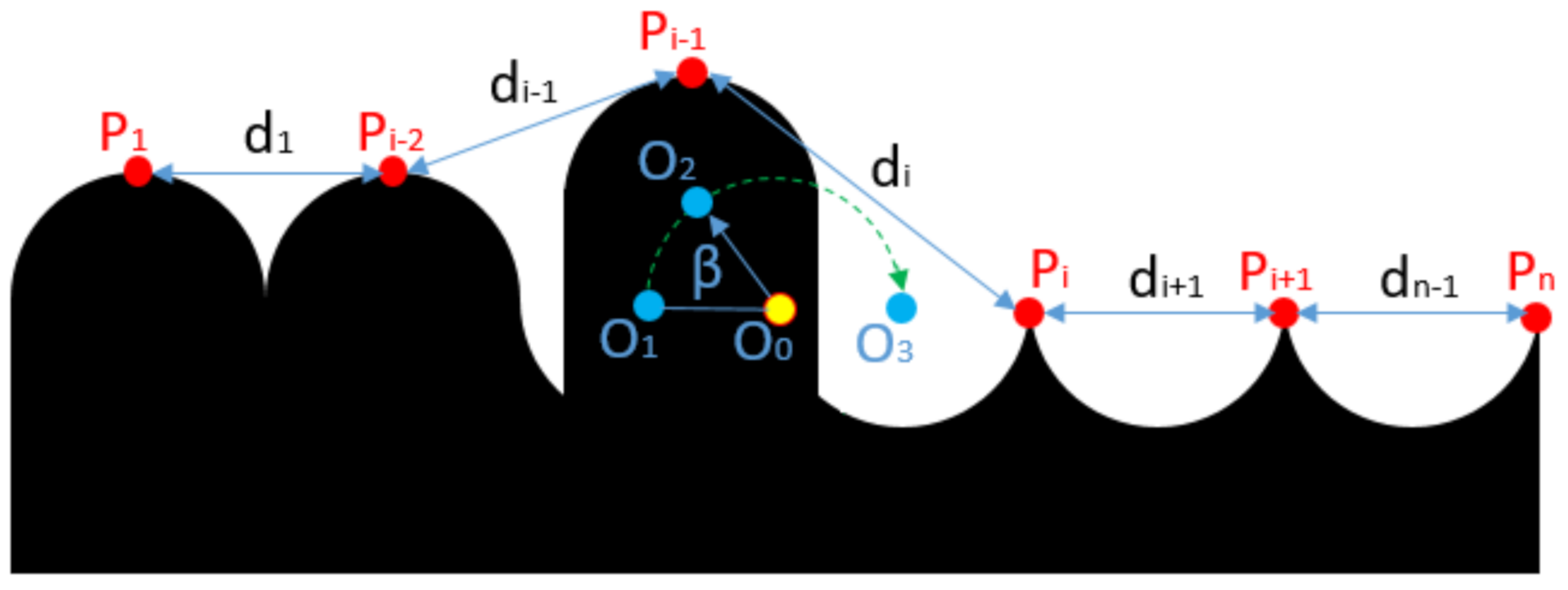
| diff() | A function of differential algorithm | The central circle projection of the torus | P | Points of eigenvalues | |
| sign() | A function to extract symbols | The external projection of the ring | d | Distance between points of eigenvalues | |
| abs() | A function to calculate the absolute value | The angle between the projection light and the plane of the central circle of the torus | The skip angle |
| η (%) | |||
|---|---|---|---|
| 50 | 7.20 | 8.81 | 10.19 |
| 60 | 10.68 | 12.96 | 15.00 |
| 70 | 16.95 | 20.91 | 24.07 |
| 80 | 31.83 | 39.24 | 45.47 |
| Drum’s Width | Drum’s Diameter | Light Source’s Distance | Rope’s Diameter | Number of Rope Winding | η | Camera Resolution | Camera Frame Rate | |
|---|---|---|---|---|---|---|---|---|
| 0.5 m | 0.3 m | 10 m | 0.005 m | 95 | 60 | 70% | 1920 × 1680 | 60 fps |
| Videos | Total Frames | Image Size (Pixel × Pixel) | Row Rope Wrong? | Error Sequences | Error Sequence Prediction | Detection Time (s) | Detection Speed (fps) |
|---|---|---|---|---|---|---|---|
| Video 1 | 2700 | 730 × 50 | No | \ | None | 11.8 | 228 |
| Video 2 | 2399 | 1700 × 211 | No | \ | None | 25.5 | 94 |
| Video 3 | 1199 | 1347 × 110 | Yes | 1–857 | 1–857 | 7.8 | 153 |
| Video 4 | 2159 | 1347 × 110 | Yes | (1) 567–1427 (2) 1429–2159 | (1) 565–1427 (2) 1427–2159 | 14.1 | 153 |
| Drum’s Width | Drum’s Diameter | Light Source’s Distance | Rope’s Diameter | Number of Rope Winding | η | Camera Resolution | Camera Frame Rate | |
|---|---|---|---|---|---|---|---|---|
| 0.15 m | 0.8 m | 3.5 m | 0.01 m | 14 | 80 | 70% | 1920 × 1680 | 60 fps |
| Videos | Total Frames | Image Size (Pixel × Pixel) | Row Rope Wrong? | Error Sequences | Error Sequence Prediction | Detection Time (s) | Detection Speed (fps) |
|---|---|---|---|---|---|---|---|
| Video 5 | 3565 | 470 × 70 | No | \ | None | 11.5 | 310 |
| Video 6 | 5585 | 462 × 70 | Yes | 1128–3423 | 1126–3423 | 17.1 | 326 |
Publisher’s Note: MDPI stays neutral with regard to jurisdictional claims in published maps and institutional affiliations. |
© 2021 by the authors. Licensee MDPI, Basel, Switzerland. This article is an open access article distributed under the terms and conditions of the Creative Commons Attribution (CC BY) license (http://creativecommons.org/licenses/by/4.0/).
Share and Cite
Shi, L.; Tan, J.; Xue, S.; Deng, J. Inspection Method of Rope Arrangement in the Ultra-Deep Mine Hoist Based on Optical Projection and Machine Vision. Sensors 2021, 21, 1769. https://doi.org/10.3390/s21051769
Shi L, Tan J, Xue S, Deng J. Inspection Method of Rope Arrangement in the Ultra-Deep Mine Hoist Based on Optical Projection and Machine Vision. Sensors. 2021; 21(5):1769. https://doi.org/10.3390/s21051769
Chicago/Turabian StyleShi, Lixiang, Jianping Tan, Shaohua Xue, and Jiwei Deng. 2021. "Inspection Method of Rope Arrangement in the Ultra-Deep Mine Hoist Based on Optical Projection and Machine Vision" Sensors 21, no. 5: 1769. https://doi.org/10.3390/s21051769