1. Introduction
With the rapid development of robotics and artificial intelligence technology, robots are increasingly used in many industrial applications, such as automobile manufacturing, mechanical processing, electrical and electronic industries, rubber and plastic industries, etc. Compared with the 6-DOF manipulator, a redundant manipulator with unique self-motion characteristics can accomplish complicated tasks easily, such as obstacle avoidance, singularity avoidance, and torque optimization [
1]. The stiffness of the redundant manipulator decreases with the increase of the number of axes, so the 7-DOF manipulator, which is considered the simplest redundant manipulator, attracts the attention of scholars [
2,
3].
For redundant manipulators’ kinematic problems, a challenging problem is how to select an appropriate solution because the number of inverse kinematics solutions is infinite. Usually, the following methods are used: geometric method [
4]; numerical method [
5,
6,
7], such as pseudo-inverse of Jacobian matrix [
8], augmented Jacobian matrix [
9,
10], gradient projection method [
11], weighted least-norm solution [
12], etc. The kinematic control of redundant manipulators can be achieved by position-based or velocity-based methods. Additionally, the latter is considered the standard approach to derive the inverse kinematics expression of the redundant manipulator [
13]. However, compared with the position-based solution, the velocity-based solution exhibits several disadvantages, such as returning only one solution [
14,
15], requiring the pre-assignment of Cartesian trajectory, accumulation error, etc. [
16] Since the number of inverse kinematics solutions of the redundant robot arm is infinite, the position-based closed-form solution is difficult to derive. Usually, the aided parameter, such as redundant angle, is introduced to derive the expression of inverse kinematics [
17]. However, how to choose the appropriate joint angle needs to be researched further. A method about the comparison of the workspace proposed by Zaplana et al. is used to solve the problem about the selection of the redundant angle [
18]. An elbow angle method with a more obvious geometric meaning is proposed by Kreutz-Delgado et al. [
19], which can select the value of the redundant parameters according to the task. A position-based control method for the KUKA LBR (A commercial 7-DOF manipulator from KUKA Corporation) manipulator is proposed by Faria [
16], and its configuration is an SRS (spherical joint, revolute joint, spherical joint) humanoid manipulator. Two auxiliary parameters are introduced to deal with the self-motion manifolds, the inverse kinematics is obtained by the geometric method, and the singularity avoidance is analyzed.
The singularity analysis and avoidance are very important for the path planning and movement control of redundant manipulators [
20,
21]. The Jacobian matrix for the redundant manipulator is a non-square matrix; the singularity condition cannot be obtained by simply finding the determinant of the matrix, so it is difficult to solve it. The Gram–Schmidt decomposition of the Jacobian matrix was used by Podhorodeski et al. [
22] to solve the singular configurations of the redundant manipulator with a spherical wrist. Nokleby et al. [
23] proposed a method based on screw reciprocity, which can be regarded as a general method for the singularity analysis of redundant manipulators. Kong et al. [
24] proposed an approach of dependent-screw suppression to analyze the singularity of a 7-DOF redundant manipulator Canadarm2. Xu et al. [
25,
26] discussed the singularity condition of Canadarm2 by using the elementary matrix of Jacobian. To solve the singularity avoidance problem, the general methods are damped least variance (DLS) [
27], singular value decomposition (SVD) [
25], singular consistency method [
28], and singular robustness algorithm [
29]. However, most of these singularity avoidance algorithms are analyzed based on velocity and generally determine whether a singularity occurs during motion by computing the rank of the Jacobian matrix, while the position-based singular avoidance method in the case of deriving redundant robot inverse kinematics analytic solutions has not been discussed. That is, the position of the end-effector and the position of the joint angle are used to determine whether the manipulator is in a singular configuration.
The optimum kinematic design for a 7-DOF SRS configuration serial manipulator was proposed by Hollerbach [
30], Due to its structural advantages in task performance and anthropomorphic characteristics, it has been extensively studied [
31,
32]. There are also many studies on the kinematics and singularity of a complex space manipulator with distance offset (the axes of the spherical joints do not intersect) [
33,
34]. Another superior kinematic design is a 7-DOF redundant manipulator with three consecutive parallel axes, which differs from the SRS configuration series manipulator in that the axis direction of joint 3 is different. There is little research on the kinematics and singularity of such a three consecutive parallel axes 7-DOF redundant manipulator.
In this paper, the kinematics and singularities of a typical 7-DOF manipulator with three consecutive parallel axes without distance offset are researched. The auxiliary parameters of its inverse kinematics are determined by self-motion analysis, and the analytical solution of its inverse kinematics is obtained. The singularity of this manipulator and the singular avoidance are studied.
2. Kinematics
2.1. Forward Kinematics
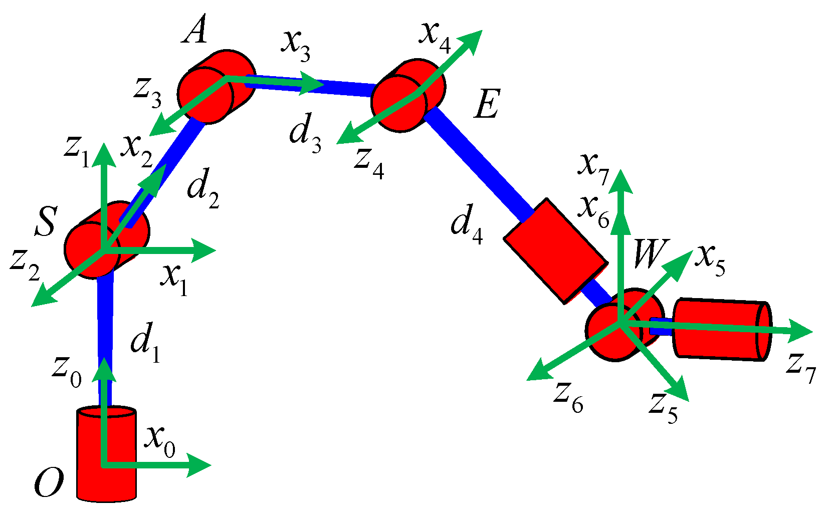
The robot that is researched is composed of seven revolute joints with three consecutive parallel axes. To realize kinematic control and describe the kinematic relationship between the pose of the robot’s end-effector and joint angle, the mechanical structure and joint coordinate system of this manipulator are shown in
Figure 1.
The base coordinate frame is fixed to the ground, and each joint coordinate frame is defined based on D–H rules. To simplify the mathematical model, the tool coordinate system is not considered. The D–H parameters of the manipulator are presented in
Table 1, in which the length of each link is
d1 = |
OS|,
d2 = |
SA|,
d3 = |
AE|,
d4 = |
EW|.
According to the D–H rules and parameters of this manipulator listed in
Table 1, the coordinate transform matrix of adjacent joints can be obtained by using a homogeneous transformation matrix
.
where
,
,
,
.
When the values of all joint angles are known, the homogeneous transformation matrix of the end-effector relative to the base can be obtained by multiplying seven homogeneous transformation matrices.
According to Equation (2) the forward kinematic solution can be obtained, which indicates the position and orientation of the end-effector.
2.2. Self-Motion Analysis
According to the mechanical characteristics of the manipulator, the geometric simplification of the manipulator is carried out. Since the axes of the last three joints of the manipulator intersect at a point, when the axes are not coplanar, the rotation of the axes of the last three joints corresponds to a spherical pair centered on
W, as shown in
Figure 2.
When the position of the end-effector is determined, the location of
W is known. Since the axes of the joints 2, 3, 4 are parallel to each other and the locations of point
O and point
S remain unchanged, it can be known that point
O,
S,
A,
E, and
W are on the same plane
P and the possible motion of the manipulator is the movement of the links
SA,
AE, and
EW on the plane
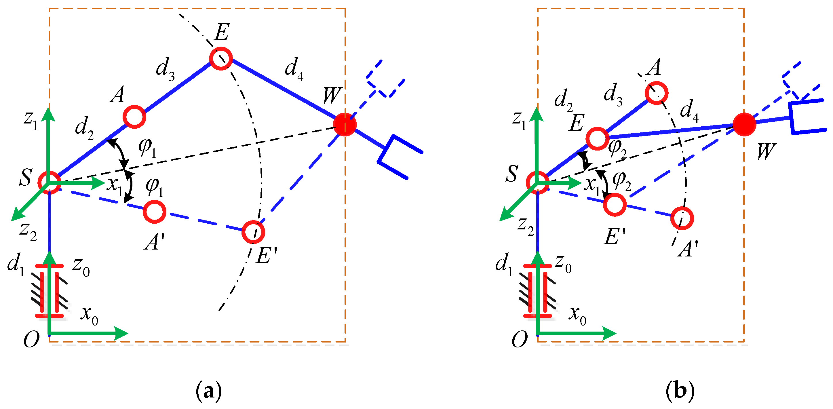
P. It can be considered as the self-motion of the 7-DOF manipulator. The movement can be seen as the planar four-bar motion with SW as the fixed link. The positions of points
A and
E are determined by only one parameter. The angle
φ between
SA and
SW is considered as the parameter of the self-motion, as shown in
Figure 3.
When the end-effector of the manipulator is at a different position, the length of SW is different. The variation range of redundant angle φ can be derived according to the kinematic principle of planar four-bar mechanism, which lays a foundation for solving the inverse kinematics of the redundant manipulator based on the redundant angle φ.
2.3. Inverse Kinematics
According to the configuration characteristics of this manipulator, the last three joints of the manipulator are equivalent to a spherical joint, which can reach any orientation. Therefore, for the inverse kinematics, the separation of position and orientation can be achieved. In this way, the first four joints of the manipulator determine the position of the end-effector; the last three joints determine the orientation of the end-effector.
Assuming the position and orientation of the manipulator are known as
The inverse kinematics can be solved by the following 5 steps:
As shown in
Figure 4, since the axes of the joints 2, 3, 4 are parallel to each other, the position of the self-motion plane
P is only determined by joint 1. Therefore, the expression of
θ1 is
where
GK1= ±1 corresponding to the two solutions of
θ1,
n0 and
z1 is the axis direction of the joint 1 in the base coordinate system,
n0 and
n1 are the normal vectors of the initial principal plane
P’ and the corresponding principal plane
P of the current point
W.
where
As shown in
Figure 5,
θ2 can represent the angle of rotation from
x1 to
x2 around
z2, and
x2 is collinear with the link
SA. If the redundancy angle
φ is known,
θ2 can be expressed as
where
φ is the redundant angle,
can represent the angle of rotation from
x1 to
SW around
z2.
According to
θ1,
and
z2 can be obtained.
The unit vectors z2 and x1 represent the z-axis vector of the joint axis 2 and the x-axis vector of the joint axis 1, respectively.
The position of point
A can be solved when the angles
θ1 and
θ2 are known. At this time,
AW,
AE, and
EW form a fixed triangle with a fixed edge length in
Figure 6. In this way, the position of point
E can be obtained.
where
GK2= ±1 corresponds to the two possible positions of the point
E, corresponding to point
E above and point
E’ below, respectively. |
AW| represents the distance from point
A to
W.
θ3 is the angle of rotation from
SA to
AE around
z3, so
θ3 can be expressed as follows:
According to the D–H method,
θ4 is the angle of rotation from
x3 to
x4 around
z4.
where
z2 is parallel to
z4.
X3 can be obtained by coordinate transformation according to
θ1,
θ2,, and
θ3. Because
EW and
z5 are collinear with each other,
x4 can be expressed as
According to the above analysis, the values of the first four joints have been obtained, and the transformation matrix from the initial orientation to the target orientation can be described as
where
is the orientation matrix of joint coordinate system {4} in the base coordinate system, which is calculated by
θ1,
θ2,
θ3, and
θ4.
is known and given by Equation (3).
According to the coordinate transformation of the D–H method,
is the orientation matrix of joint coordinate system {7} in coordinate system {4}, which can also be described as
where
s and
c are the abbreviations of sine function and cosine function, respectively, and the subscript number
i (
i = 1, …, 7) is the corresponding joint angle
θi. For example,
c6 = cos(
θ6).
When
, that is
. The axes of joint 5 and joint 7 of the manipulator coincide; at this time, only the sum of values of the joint 5 and the joint 7 can be obtained, and the joint angles can be arbitrarily selected as long as the sum is unchanged.
When
, that is
. Due to the existence of the cosine function, there are two solutions. Introducing variables
GK3= ±1 reflect this position
In summary, eight discrete inverse solutions of the manipulator can be obtained with given position-orientation T and redundant angle φ, and the unique inverse solutions of the control variable GK1, GK2, and GK3 can be obtained.
3. Singularity Analysis
The Jacobian matrix reflects the mapping relationships between the generalized velocity (linear velocity and angular velocity) of the end-effector and the joint velocities. The singularity condition of the manipulator can be obtained by analyzing the conditions when the determinant of the Jacobian matrix is equal to zero. However, since the Jacobian matrix of the redundant manipulator is not a square matrix, it is not feasible to obtain singular conditions by means of the matrix determinant. The method based on the elementary transformation [
26] of the Jacobian matrix is widely used. That is, the Jacobian matrix is simplified by the elementary transformation. The singular conditions are analyzed and concentrated in a low-dimensional submatrix by the form of the block matrix, and then the singularity conditions of the submatrix are analyzed to obtain the singularity conditions of the entire Jacobian matrix [
23].
3.1. Jacobian Matrix
In this paper, the vector cross-product method [
35] is used to establish the Jacobian matrix of the manipulator. The relationship between the terminal velocity and the joint velocity corresponding to a single joint is as follows:
where
ω and
v are the angular velocity and linear velocity of the end effector, respectively.
is the joint velocity vector and
J(
θ) is the Jacobian matrix. Since the seven joints of this manipulator are all revolute joints, the
ith column of the Jacobian matrix can be expressed as:
where
zi is the unit vector of the
ith joint axis,
is the representation of the origin of the joint coordinate system {7} in the joint coordinate system {5} relative to the position vector in the coordinate system {
i}.
Adopting the above method, the Jacobian matrix of the manipulator is established with joint 5 as the reference coordinate system as follows:
where the subscript of the symbol represents the sine or cosine of the corresponding joint variable sum, such as
.
Because of the wrist structure of the manipulator, the last three columns of the Jacobian matrix are in the simplest form. In this way, the Jacobian matrix can be separated into a low-dimensional matrix by elementary transformation. In the following section, the expression of the low-dimensional matrix is expressed, and the singularity conditions of the Jacobian matrix are obtained by analyzing the singularity conditions of the matrix.
3.2. Singularity Conditions
According to Equation (19), the lower right corner of the Jacobian matrix is simplified to a 3 × 3 zero matrix, which can be discussed by dividing the Jacobian matrix into blocks. The following discussion is based on the value of S6:
When
S6 = 0, the Jacobian matrix can be transformed into the following form
where
λ1 to
λ6 in Equation (20) are sub-matrices of the Jacobian matrix to make the structure of the Jacobian matrix look more concise.
To facilitate the singularity analysis, elementary transformation is performed on the matrix in Equation (20), and the matrix is written into the form of a block matrix.
where
is a 4 × 3 zero matrix, and the other sub-matrices are as follows:
According to the characteristics of the matrix rank,
is a row full rank matrix, i.e.,
. So, the rank of the block-triangle matrix can be computed according to the following equation [
36]:
If
is singular, it should satisfy:
We only need to analyze the singularity
.
where
Since
is a square matrix, the singularity conditions of the Jacobian matrix can be obtained by judging whether the determinant of the matrix is equal to zero.
Then, it can be obtained that, when , the rank of the Jacobian matrix is less than 6; that is, it is in the singular position. For , there are three cases: , , and .
When
S6 ≠ 0, the Jacobian matrix can be expressed in the form of block matrix
where
is a square matrix and its determinant value is
. Because of
S6 ≠ 0, to make Jacobian matrix singular, it needs to satisfy
The singularity of the Jacobian matrix can be judged by analyzing the singularity of
. The expression of
is as follows:
where
Since the matrix is a rectangular matrix, the determinant method cannot obtain the condition of matrix rank deficiency. Therefore, it is necessary to be discussed according to the structural characteristics of the matrix. By looking at the first column of matrix , we can see the following:
Since , S6 ≠ 0 and is one of the conditions of matrix rank deficiency. Consider Equation (27), S6 = 0 and is also one of the conditions of matrix rank deficiency. Therefore, is one of the singular conditions of the matrix regardless of whether S6 is equal to 0 or not.
If
S5 = 0, then the matrix can be written in the following form after the elementary transformation:
It can be seen that the value of joint 5 does not affect the rank of the matrix, so the only condition in which the rank of the matrix
is not full is
In summary, there are four singularity conditions for the 7-DOF redundant manipulator, as shown in
Table 2. If the joint angles of the manipulator satisfy any of them, the manipulator will be in a singular configuration.
4. Singularity Avoidance
It can be seen from the above analysis that the singularity conditions are described in the joint space. However, in practice, the end-effector of this manipulator is usually planned, and the singularity configuration is impossible to be predicted and avoided in motion planning because of the infinite number of the inverse kinematics solutions of the redundant manipulator. In the following section, the above-mentioned singular configuration is described based on position, and a singularity avoidance method is proposed for the avoidable singularities.
4.1. Type I Singularity
According to the expression analysis of condition 1 and condition 2, there are four possible configurations of manipulators regarding condition 1, which are shown in
Table 3, and the configurations regarding condition 2 are shown in
Table 4.
The first two of the four singularity conditions described above are all related to joint 6, so both condition 1 and condition 2 can be regarded as the first type of singularity. Since both condition 1 and condition 2 contain S6 = 0, such singular problems can be solved by avoiding the configuration corresponding to S6 = 0 through self-motion.
The following is the analysis of the characteristics of the manipulator when
S6 = 0. When
S6 = 0, the rotation axes of the joints 5 and 7 coincide with each other, and, since the axes of joints 2, 3, and 4 are parallel to each other, the axes of joints 5 and 7 must also be in the self-motion plane
P formed by joints 2, 3, and 4, as shown in
Figure 7.
Since the axis of the last joint 7 lies on the main plane
P, according to the Equations (3) and (5), it can be expressed as
where
,
n1 is the normal vector to the plane
P. Simplified Equation (35) can be obtained:
When the singularity occurs in
Table 3, according to the geometric theorem forming the triangle, the distance
SW between the shoulder point and wrist point of the manipulator and the corresponding redundancy angle meet the following equation:
where the angle ±
φ1 represents the corresponding redundancy angle when singular conditions of
θ3 = 0,
θ6 = 0, or π are satisfied, as shown in
Figure 7a. In this case, angle
φ1 can be expressed as the following equation:
where the distance of
SW can calculated from a given end-effector position, i.e., Equation (6). At this point, the axis vector of joint 5 (i.e., vector
EW or
E’W) can be expressed as:
where
represents the rotation matrix for the rotation of angle ±
φ1 about the
z2 axis. The angle ±
φ2 represents the corresponding redundancy angle when singular condition of
θ3 = π,
θ6 = 0, or π are satisfied, as shown in
Figure 7b. In this case, angle
φ2 can be expressed as the following equation:
So, the axis vector of joint 5 can be expressed as:
When the axis of joint 7 is collinear with
EW or
E’W, the following equation is satisfied:
Therefore, when the position and orientation of the end-effector are given, the relationship between EW vector and the axis vector a of joint 7 can be determined to know whether the manipulator is in the singular pose corresponding to singular condition 1.
In order to avoid singular configuration corresponding to singular condition 1, the redundant angle φ obtained according to Equation (38) and Equation (40) should be avoided during motion planning. However, singular condition 2 is only related to joint 5 and joint 6, and this singular type cannot be determined by the given end-effector position and orientation.
4.2. Type II Singularity
The last two of the four singularity conditions are related to joints 2, 3, and 4, so both conditions 3 and 4 can be regarded as the second kind of singularity. Since the first four joints determine the position of the end-effector, they can be regarded as the position singularity. From the perspective of workspace, position singularity can be divided into boundary singularity and internal singularity. Boundary singularity refers to the singularity caused by the position of the end-effector at the boundary of the workspace. Internal singularity refers to the position of the end-effector in the workspace when it is in the singular configuration. Whether it can be avoided needs to be discussed.
According to the geometric projection relationship of
Figure 8, the projection of point
W in the horizontal direction
x is shown in Equation (43).
where
. When this condition
is satisfied, that is, singular condition 3, its geometric meaning is that the projection of point
W in the horizontal direction
x is zero. In other words, the end-effector of the manipulator is located on the axis of joint 1. At the moment, the position of the end-effector of the manipulator satisfies
From the analysis of the working space, the end-effector of the manipulator loses the movement perpendicular to the normal direction of the main plane, so the axis of joint 1 is also the boundary of the working space and cannot be avoided, as shown in
Figure 9.
According to the expression analysis of condition 4, there are four possible joint combinations of joint 3 and joint 4, as shown in
Table 5.
When
θ3 = 0,
θ4 = π/2, the manipulator is in the singularity position of the boundary of the workspace, which is an unavoidable singularity, and the other three are internal singularities. These four configurations have common motion characteristics. In these cases, points
S and
W are on a straight line; the length of
SW is as follows:
At this time, the corresponding redundancy angle is φ = 0. Therefore, it can be concluded that, when the end-effector of the manipulator is in the avoidable singularity, the control variable φ is unequal to zero to avoid the current singularity configuration.


