
A Novel Low-Cost Instrumentation System for Measuring the Water Content and Apparent Electrical Conductivity of Soils

Abstract
:1. Introduction
2. Experimental Setup
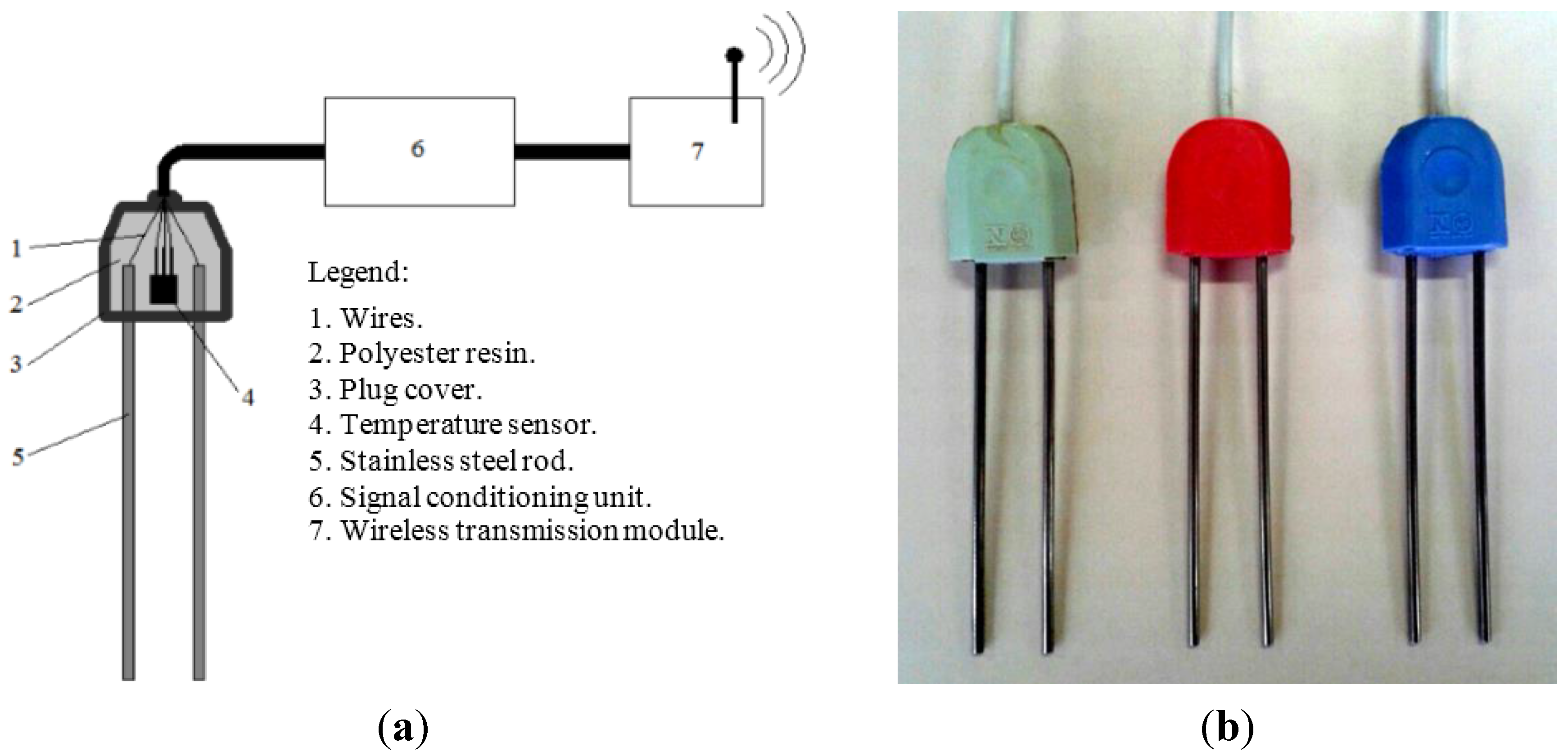
2.1. Probes for Measuring θ, σ and T
2.2. Theory and Signal Conditioning Unit


2.3. Calibration and Testing
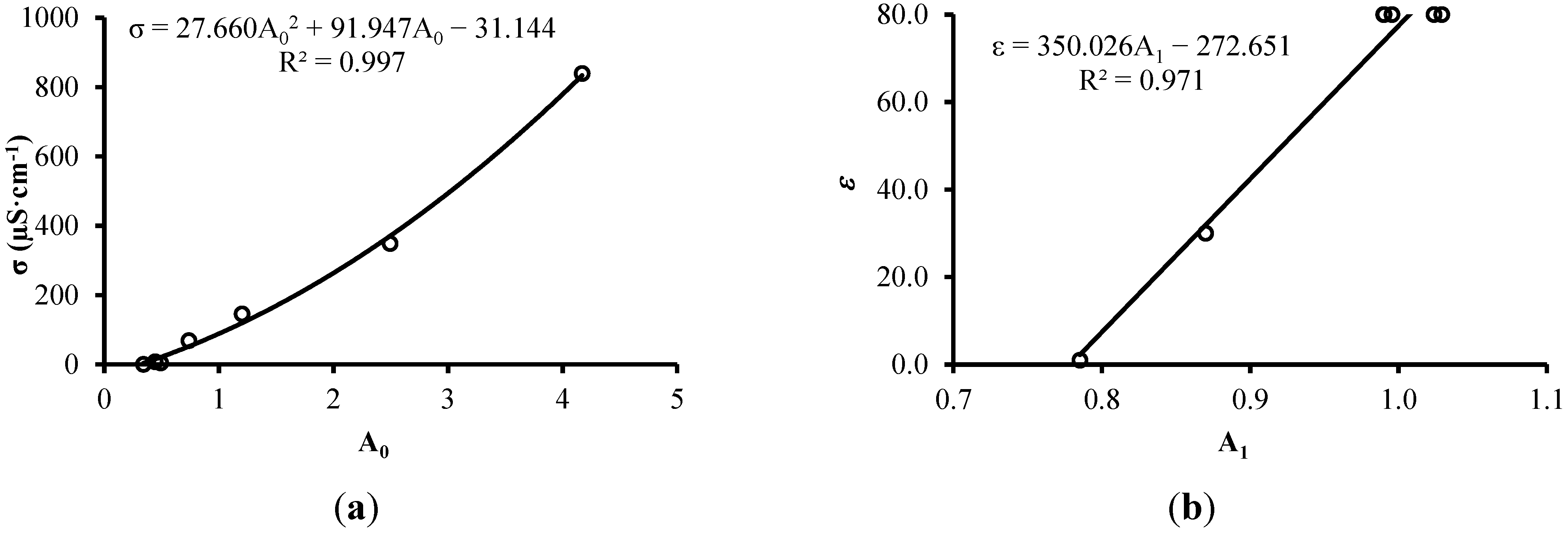
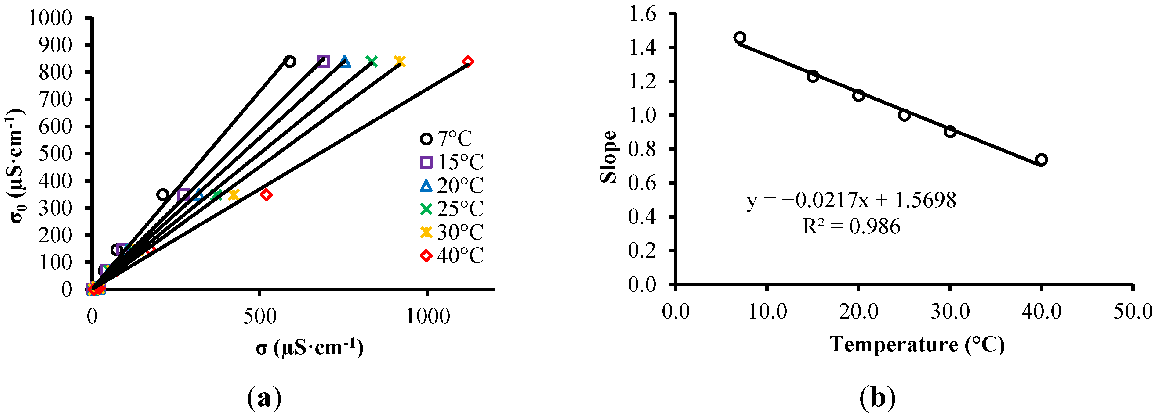
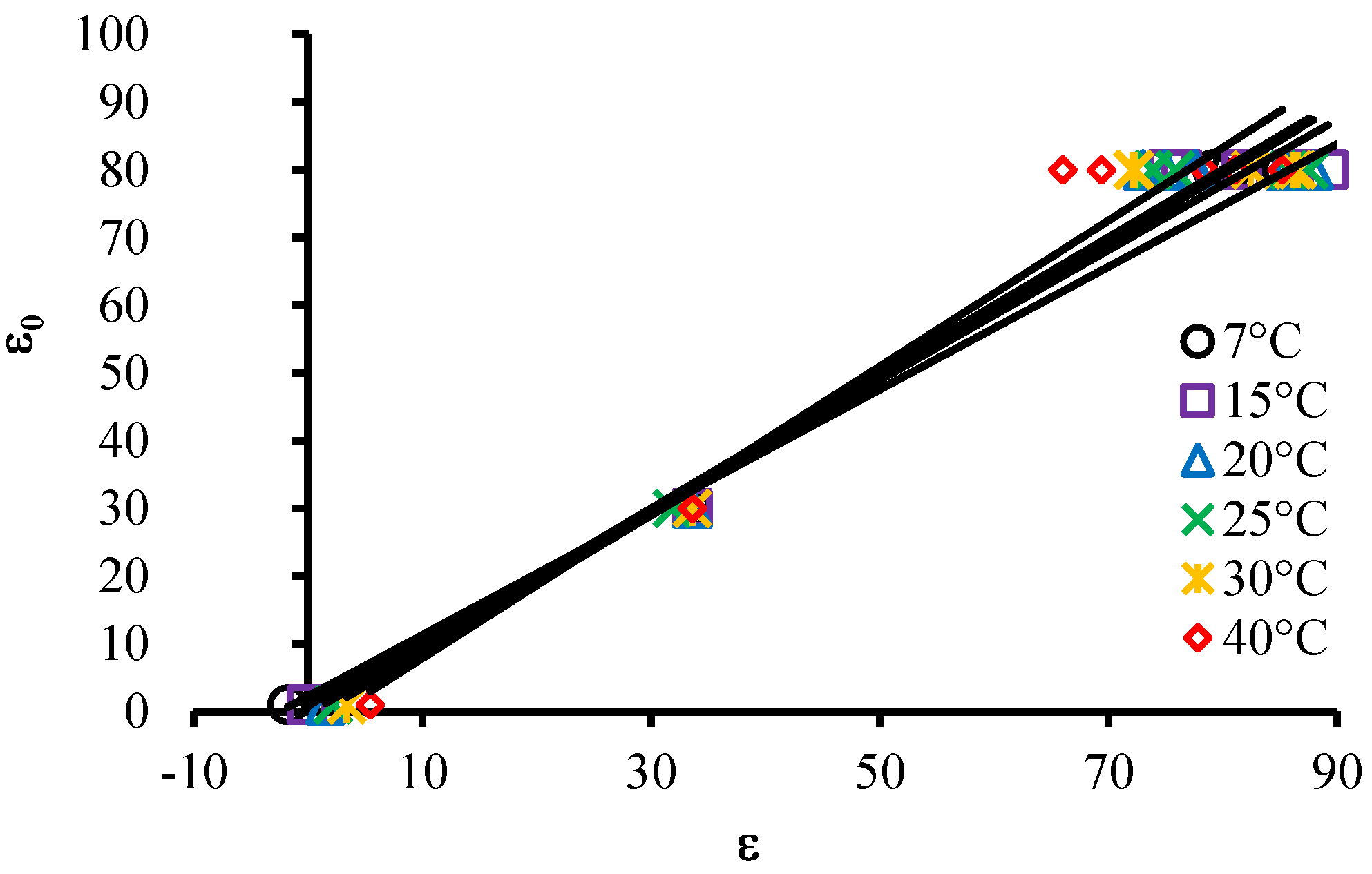
2.3.1. Calibration Using Salts Solutions
- Air ;
- Deionized water.
- Drinking water.
- Solution of water and NaCl 1
- Solution of water and NaCl 2
- Solution of water and NaCl 3
- Ethanol fuel
2.3.2. Tests Conducted with Soil

3. Results and Discussion
3.1. Salt Solutions


3.2. Soils


| Sandy Soil | Clay Soil | |||
|---|---|---|---|---|
| RMSE | R2 | RMSE | R2 | |
| No correction | 6.7727 | 0.9321 | 1.9827 | 0.9598 |
| Equation 12 | 0.9676 | 0.9986 | 1.0620 | 0.9886 |
| Rhoades et al. | 1.3751 | 0.9971 | 0.7929 | 0.9936 |

| Linear Regression | Cross-Validation | ||
|---|---|---|---|
| R2 | R2 | Standard Deviation | |
| Equation (14) | 0.9866 | 0.9856 | 0.0003 |
| Equation (15) | 0.9850 | 0.9839 | 0.0003 |
| Equation (16) | 0.9323 | 0.9298 | 0.0007 |
| Sandy Soil | Clay Soil | |||
|---|---|---|---|---|
| RMSE | R2 | RMsSE | R2 | |
| Topp et al. | 0.05176 | 0.9319 | 0.02839 | 0.8798 |
| Lidieu et al. | 0.04613 | 0.9542 | 0.2374 | 0.9191 |
| Malicki et al. | 0.05114 | 0.9542 | 0.02334 | 0.9191 |
| Equation (14) | 0.01455 | 0.9866 | - | - |
| Equation (15) | - | - | 0.01001 | 0.9850 |
| Equation (16) | 0.03584 | 0.9804 | 0.02078 | 0.9797 |

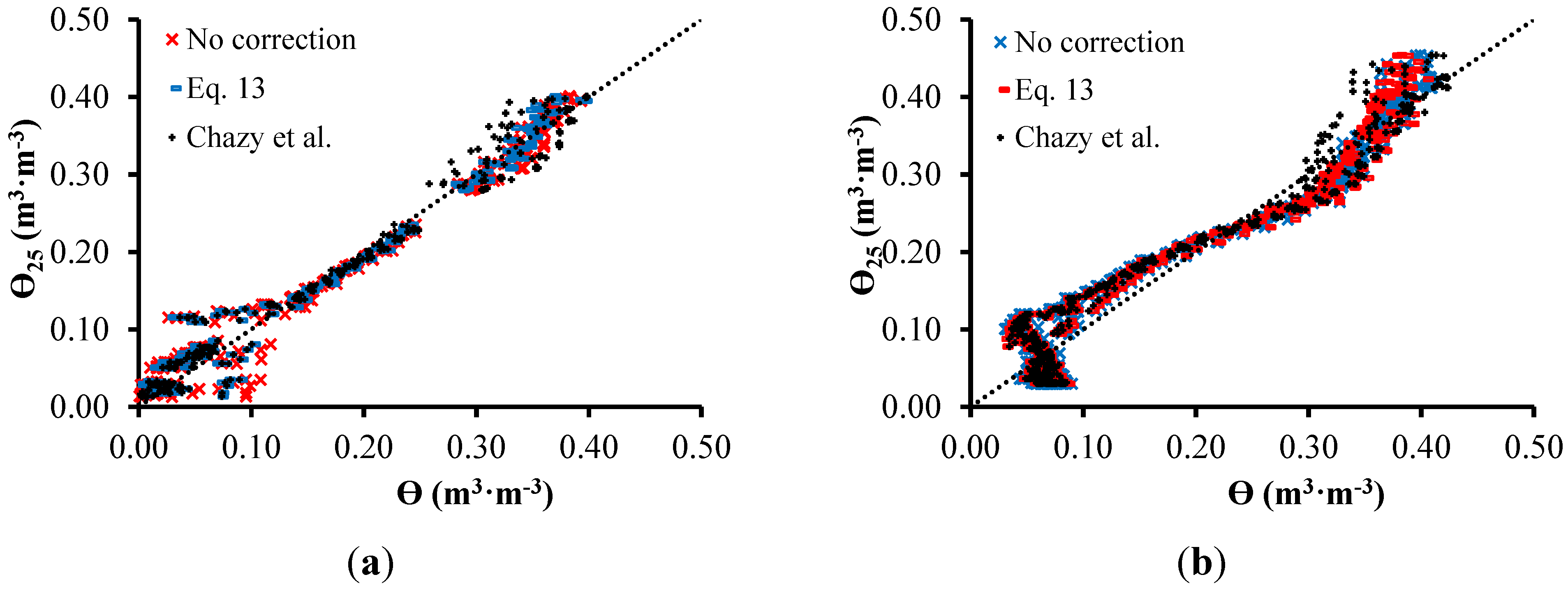
| Sandy Soil | Clay Soil | |||
|---|---|---|---|---|
| RMSE | R2 | RMSE | R2 | |
| No correction | 0.02322 | 0.9713 | 0.03232 | 0.9381 |
| Equation (9) | 0.02215 | 0.9761 | 0.03250 | 0.9380 |
| Chanzy et al. | 0.02250 | 0.9704 | 0.03273 | 0.9367 |
4. Conclusions
Acknowledgments
Author Contributions
Conflicts of Interest
References
- United Nations Educational, Scientific and Cultural Organization. Launch Water Cooperation 2013. Available online: http://www.unesco.org/new/en/natural-sciences/environment/water/water-cooperation-2013/launch-water-cooperation-2013/ (accessed on 7 June 2015).
- Corwin, D.L.; Lesch, S.M. Application of soil electrical conductivity to precision agriculture: Theory, principles, and guidelines. Agron. J. 2003, 95, 455–471. [Google Scholar] [CrossRef]
- Ash, C.; Jasny, B.R.; Malakoff, D.A.; Sugden, A.M. Food security, feeding the future, introduction. Science 2010, 327, 797. [Google Scholar] [CrossRef] [PubMed]
- Rêgo Segundo, A.K.; Martins, J.H.; Marcos de Barros Monteiro, P.; Alves de Oliveira, R. Monitoring System of Apparent Electrical Conductivity and Moisture Content of Soil for Controlling of Irrigation Systems. In Proceedings of the International Conference of Agricultural Engineering—AgEng 2014, Zurich, Switzerland, 6–10 September 2014.
- Corwin, D.L.; Lesch, S.M. Protocols and Guidelines for Field-scale Measurement of Soil Salinity Distribution with ECa-Directed Soil Sampling. J. Environ. Eng. Geophys. 2013, 18, 1–25. [Google Scholar] [CrossRef]
- Hedley, C.B.; Roudier, P.; Yule, I.J.; Ekanayake, J.; Bradbury, S. Soil water status and water table depth modelling using electromagnetic surveys for precision irrigation scheduling. Geoderma 2013, 199, 22–29. [Google Scholar] [CrossRef]
- Hedley, C.B.; Yule, I.J. Soil water status mapping and two variable-rate irrigation scenarios. Precis. Agric. 2009, 10, 342–355. [Google Scholar] [CrossRef]
- Goumopoulos, C.; O’Flynn, B.; Kameas, A. Automated zone-specific irrigation with wireless sensor/actuator network and adaptable decision support. Comput. Electron. Agric. 2014, 105, 20–33. [Google Scholar] [CrossRef]
- Fares, A.; Polyakov, V. Advances in crop water management using capacitive water sensors. Adv. Agron. 2006, 90, 43–77. [Google Scholar]
- Wendroth, O.; Koszinski, S.; Pena-Yewtukhiv, E. Spatial association among soil hydraulic properties, soil texture, and geoelectrical resistivity. Vadose Zone J. 2006, 5, 341. [Google Scholar] [CrossRef]
- Rêgo Segundo, A.K.; Martins, J.H.; Monteiro, P.M.; Oliveira, R.A.; Oliveira Filho, D. Development of capacitive sensor for measuring soil water content. Eng. Agrícola 2011, 31, 260–268. [Google Scholar] [CrossRef]
- Bitella, G.; Rossi, R.; Bochicchio, R.; Perniola, M.; Amato, M. A novel low-cost open-hardware platform for monitoring soil water content and multiple soil-air-vegetation parameters. Sensors 2014, 14, 19639–19659. [Google Scholar] [CrossRef] [PubMed]
- Scudiero, E.; Berti, A.; Teatini, P.; Morari, F. Simultaneous monitoring of soil water content and salinity with a low-cost capacitance-resistance probe. Sensors 2012, 12, 17588–17607. [Google Scholar] [CrossRef] [PubMed]
- Pelletier, M.G.; Karthikeyan, S.; Green, T.R.; Schwartz, R.C.; Wanjura, J.D.; Holt, G.A. Soil moisture sensing via swept frequency based microwave sensors. Sensors 2012, 12, 753–767. [Google Scholar] [CrossRef] [PubMed]
- Kizito, F.; Campbell, C.S.; Campbell, G.S.; Cobos, D.R.; Teare, B.L.; Carter, B.; Hopmans, J.W. Frequency, electrical conductivity and temperature analysis of a low-cost capacitance soil moisture sensor. J. Hydrol. 2008, 352, 367–378. [Google Scholar] [CrossRef]
- Thalheimer, M. A low-cost electronic tensiometer system for continuous monitoring of soil water potential. J. Agric. Eng. 2013, 44, 16. [Google Scholar] [CrossRef]
- Dias, P.C.; Roque, W.; Ferreira, E.C.; Siqueira Dias, J.A. A high sensitivity single-probe heat pulse soil moisture sensor based on a single npn junction transistor. Comput. Electron. Agric. 2013, 96, 139–147. [Google Scholar] [CrossRef]
- Vellidis, G.; Tucker, M.; Perry, C.; Kvien, C.; Bednarz, C. A real-time wireless smart sensor array for scheduling irrigation. Comput. Electron. Agric. 2008, 61, 44–50. [Google Scholar] [CrossRef]
- Gardner, C.M.K.; Dean, T.J.; Cooper, J.D. Soil Water Content Measurement with a High-Frequency Capacitance Sensor. J. Agric. Eng. Res. 1998, 71, 395–403. [Google Scholar] [CrossRef]
- Seyfried, M.S.; Murdock, M.D. Measurement of Soil Water Content with a 50-MHz Soil Dielectric Sensor. Soil Sci. Soc. Am. J. 2004, 68, 394. [Google Scholar] [CrossRef]
- Rêgo Segundo, A. K. SISTEMA DE MONITORAMENTO DO SOLO E DE CONTROLE DE IRRIGAÇÃO. BR Patent BR1020130132209, 28 May 2013. [Google Scholar]
- Vidovich, N.V. Area Soil Moisture and Fertilization Sensor. U.S. Patent US20130073097 A1, 21 March 2013. [Google Scholar]
- Charles, M. Soil Moisture Sensing System. U.S. Patent US3882383 A, 6 May 1975. [Google Scholar]
- Feuer, L. Soil Moisture Sensor. U.S. Patent US5445178 A, 29 August 1995. [Google Scholar]
- Da Silva, M.J. Impedance Sensors for Fast Multiphase Flow Measurement and Imaging. Ph.D. Thesis, Technische Universität Dresden, Dresden, Germany, 08 November 2008. [Google Scholar]
- Kaatze, U.; Feldman, Y. Broadband dielectric spectrometry of liquids and biosystems. Meas. Sci. Technol. 2006, 17, R17–R35. [Google Scholar] [CrossRef]
- Okada, K.; Sekino, T. The Impedance Measurement Handbook—A Guide to Measurement Technology and Techniques; Agilent Technologies, Inc.: Santa Clara, CA, USA, 2003. [Google Scholar]
- Agilent Technologies. Basics of Measuring the Dielectric Properties of Materials—Application Note; Agilent Technologies, Inc.: Santa Clara, CA, USA, 2006. [Google Scholar]
- Cambell, J.E. Electrical Sensor for Determining the Moisture Content of Soil. U.S. Patent US5479104, 26 December 1995. [Google Scholar]
- Watson, K.; Gatto, R.; Weir, P.; Buss, P. Moisture and Salinity Sensor and Method of Use. U.S. Patent US5418466 A, 23 May 1995. [Google Scholar]
- Delta-T Devices: Soil Moisture Content, Pyranometers, Data Loggers, Canopy Analysis. Available online: http://www.delta-t.co.uk/default.asp (accessed on 7 June 2015).
- CD620: Display for the Hydrosense® System. Available online: http://www.campbellsci.com/cd620 (accessed on 17 June 2015).
- IMKO GmbH—Precise Moisture Measurement. Available online: http://www.imko.de/ (accessed on 17 June 2015).
- Gregory, A.P.; Clarke, R.N. A review of RF and microwave techniques for dielectric measurements on polar liquids. IEEE Trans. Dielectr. Electr. Insul. 2006, 13, 727–743. [Google Scholar] [CrossRef]
- Yang, W.Q.; York, T.A. New AC-based capacitance tomography system. IEE Proc. Sci. Meas. Technol. 1999, 146, 47–53. [Google Scholar] [CrossRef]
- Georgakopoulos, D.; Yang, W.; Waterfall, R. Best value design of electrical tomography systems. In Proceedings of the 3rd World Congress on Industrial Process Tomography, Banff, AB, Canada, 2003; pp. 11–19.
- Rhoades, J.; Chanduvi, F.; Lesch, S. Soil Salinity Assessment: Methods and Interpretation of Electrical Conductivity Measurements; FAO: Riverside, CA, USA, 1999. [Google Scholar]
- Chanzy, A.; Gaudu, J.-C.; Marloie, O. Correcting the temperature influence on soil capacitance sensors using diurnal temperature and water content cycles. Sensors 2012, 12, 9773–9790. [Google Scholar] [CrossRef] [PubMed]
- Rodríguez, J.D.; Pérez, A.; Lozano, J.A. Sensitivity analysis of kappa-fold cross validation in prediction error estimation. IEEE Trans. Pattern Anal. Mach. Intell. 2010, 32, 569–75. [Google Scholar] [CrossRef] [PubMed]
- Topp, G.; Davis, J.; Annan, A. Electromagnetic determination of soil water content: Measurements in coaxial transmission lines. Water Resour. Res. 1980, 16, 574–582. [Google Scholar] [CrossRef]
- Ledieu, J.; de Ridder, P.; de Clerck, P.; Dautrebande, S. A method of measuring soil moisture by time-domain reflectometry. J. Hydrol. 1986, 88, 319–328. [Google Scholar] [CrossRef]
- Malicki, M.; Plagge, R.; Roth, C. Improving the calibration of dielectric TDR soil moisture determination taking into account the solid soil. Eur. J. Soil 1996, 47, 357–366. [Google Scholar] [CrossRef]
- Seyfried, M.S.; Grant, L.E. Temperature Effects on Soil Dielectric Properties Measured at 50 MHz. Vadose Zone J. 2007, 6, 759. [Google Scholar] [CrossRef]
- Munoz-Carpena, R. Field devices for monitoring soil water content. Bull. Inst. Food Agric. Sci. Univ. Fla. 2004, 343, 1–16. [Google Scholar]
© 2015 by the authors; licensee MDPI, Basel, Switzerland. This article is an open access article distributed under the terms and conditions of the Creative Commons Attribution license (http://creativecommons.org/licenses/by/4.0/).
Share and Cite
Rêgo Segundo, A.K.; Martins, J.H.; Monteiro, P.M.d.B.; De Oliveira, R.A.; Freitas, G.M. A Novel Low-Cost Instrumentation System for Measuring the Water Content and Apparent Electrical Conductivity of Soils. Sensors 2015, 15, 25546-25563. https://doi.org/10.3390/s151025546
Rêgo Segundo AK, Martins JH, Monteiro PMdB, De Oliveira RA, Freitas GM. A Novel Low-Cost Instrumentation System for Measuring the Water Content and Apparent Electrical Conductivity of Soils. Sensors. 2015; 15(10):25546-25563. https://doi.org/10.3390/s151025546
Chicago/Turabian StyleRêgo Segundo, Alan Kardek, José Helvecio Martins, Paulo Marcos de Barros Monteiro, Rubens Alves De Oliveira, and Gustavo Medeiros Freitas. 2015. "A Novel Low-Cost Instrumentation System for Measuring the Water Content and Apparent Electrical Conductivity of Soils" Sensors 15, no. 10: 25546-25563. https://doi.org/10.3390/s151025546
APA StyleRêgo Segundo, A. K., Martins, J. H., Monteiro, P. M. d. B., De Oliveira, R. A., & Freitas, G. M. (2015). A Novel Low-Cost Instrumentation System for Measuring the Water Content and Apparent Electrical Conductivity of Soils. Sensors, 15(10), 25546-25563. https://doi.org/10.3390/s151025546