1. Introduction
Outdoor 3D reconstruction is a challenging aspect in many applications, such as mapping, autonomous navigation and localization, disaster control and many others. The evolution in computer science technologies, the decreasing sensor prices and the increasing number of applications referring to the 3D representation of the environmenthas pushed forward research in the field of 3d cartography of large outdoor environments. Methods existing in the literature are based on vision or range sensors or a combination of these two sensors. In this regard, a combination of sensors is an obvious solution to overcome the limitations of single sensors. Thereby, multi-sensory fusion has been recently a point of interest in widespread applications and research, especially for 3D mapping applications [
1,
2,
3].
Despite the large number of studies (a survey of 3D reconstruction is presented in [
4,
5]), there are still many challenges for fully automatic and real-time modeling processes together with high quality results, requiring more contributions. Acquiring, storing and matching processes are costly, both in terms of memory and time. Furthermore, Outdoor 3D reconstruction is a challenging aspect because of many limitations due to large-scale and unshaped features and bad illumination conditions. For these reasons, the proposal of a simple, robust and fast algorithm dedicated to complete such an objective represents a major interest for several applications. The authors in [
6] provide a comprehensive overview of urban reconstruction.
Regarding the low cost and high spatial resolution of vision sensors, a huge number of vision-based approaches for 3D reconstruction has been proposed. Methods for 3D scene reconstruction from an image sequence can be grouped into two classes: structure-from-motion and dense stereo.
SfM delivers a set of registered cameras (or poses), as well as sparse 3D point clouds (scene structure). The 3D point clouds are obtained from sparse selected feature points, which are detected in each image and then matched across the image sequence. SfM provides sparse, but accurate poses and structure. In the second step, dense matching is used for surface reconstruction. The aim is to reconstruct scene surfaces by recovering the 3D information from all pixels in contrast to sparse methods. The geometrical information obtained in the previous step is used to make the dense matching both robust and efficient. Some examples can be found in [
7,
8,
9,
10,
11,
12,
13]. In the last few years, many works intended to fill the gap between the two approaches in order to propose methods that may handle very large-scale outdoor scenes [
14,
15]. In [
16], the authors presented a new method, which is called the “mask automatic detecting method”, using a camera driving recorder, and which provided better results compared to a typical SfM method. The results seems to be of good quality, though it recommends a large amount of input data and heavy algorithms, which make it not quite suitable for real-time processing. It is also known that camera-based methods for large scene reconstruction generally suffer from scale factor drift and loop closure problems. Beside, vision sensors present common drawbacks due to the influence of image quality and adverse illumination and weather conditions. For this reason, tapping into active sensors has become essential.
The capability of range sensors to work in difficult atmospheric conditions and the decreasing cost make them well suited for extended outdoor robotic applications. For example, the authors in [
17] used a radio detection and ranging (RADAR) sensor for simultaneous localization and mapping (R-SLAM algorithm) applications in agriculture. However, the radar failed to recognize the elevation, shape, texture and size of the target. Two acquisitions from two different points of view of the same scene are often needed in order to achieve the 3D reconstruction. Many solutions based on the combination of depth and vision sensors are described in the literature. SLAM applications with Kinect are also numerous [
18,
19]. Yet, the performances for outdoor applications are generally limited due to the small depth range and sensitivity to the outdoor natural light. An example of this fusion can also be found in [
20]: an automatic classification of raw data from light detection and ranging (LiDAR) in external environments and a reconstruction of 3D models of buildings are presented. LiDAR is widely used for urban scene reconstruction; for instance, in [
21], the authors combined data from a 3D LiDAR and images to create geometric 3D models of the world. The authors in [
22], also, recently, combined six cameras and one 2D laser for urban 3D reconstruction. LiDAR provides a large number of accurate 3D points from a narrow field of view. Other examples could be found in [
23,
24]. However, the alignment of the large amount of data requires heavy processing algorithms that can be memory and time consuming. Reconstructed scenes using point cloud-based methods generally have an unstructured representation and cannot be directly represented as connected surfaces. In our method, in contrast, matches of large dimensions of surfaces (patches in the image with the target or a set of targets in the radar image) will be done, as shown, for example, in
Figure 22b,d. In addition, LiDAR is generally more expensive than radar. Furthermore, one of LiDAR’s weaknesses
versus radar is that the data acquired by LiDAR are somehow affected by the external illumination and weather conditions (like water and dust particles and also extreme sunlight). A review of the use of mobile LiDAR in several applications and of the advantages and challenges of LiDAR for city reconstruction have been summarized in [
25]. Even though radar is much less used in the literature, in particular for the 3D reconstruction, it presents several advantages for outdoor applications: radar is highly independent of the illumination and weather conditions, and several targets can be detected in the same beam thanks to the physical property of the transmitted wave. These advantages make the exploitation of radar in our system of sensors very interesting and were our first motivation to explore the combination of a panoramic millimeter wave (MMW) radar and a camera, in order to achieve a sparse 3D reconstruction of large-scale outdoor environments. Recently, this combination has been the subject of many studies so far reported in the literature, for on-road obstacle detection and vehicle tracking: in [
26], a camera and radar were integrated with an inertial sensor to perform road obstacle detection and classification.
Other works on radar-vision fusion for obstacle detection can be found in the literature [
27,
28,
29,
30]. However, we are not aware of any work using radar and a camera only, for outdoor 3D reconstruction. More than data fusion, our main objective is to build a 3D sensor that can provide textured elevation maps. Therefore, a geometrical model of the sensors and a calibration technique should be provided.
The challenge is to take full advantage of the context of data fusion, appropriately exploiting the complementarity of optical and radar sensors: we rely on the fact that the distance of an object in 3D space to the system is given by the radar measurements having a constant range error with increasing distance: with frequency modulated continuous wave (FMCW) radar, the radar to target distance is obtained with the measurement of the frequency difference between the transmitted signal and the received signal. This beat frequency is small for short distances and larger for longer distances. The distance resolution is equivalent to a frequency resolution: this frequency resolution is independent of the distance and depends on the frequency measurement performance of the data acquisition and signal processing system. For this reason, the radar uncertainty zone is constant with respect to an increasing depth.
In multi-sensor systems, each sensor performs measurements in its own coordinate system. Thus, one needs to transform these measurements into a global coordinate system. Generally, a calibration step enables one to compute this transformation in order to make the reconstruction simpler. In related works, this calibration method is not explicitly described. Sugimoto
et al. [
31] used the reflection intensity from MMW radar and image sequences to achieve a radar-vision spatial calibration. This method is hard to implement, because all of the points should be positioned exactly on the radar plane, as explained in
Section 4.1. Our goal is to simplify this tricky and important step, which is crucial for the matching process and the reconstruction accuracy. Therefore, first, we propose a technique that uses only a set of radar-to-image point matches. These points are positioned in front of the camera/radar system, and the distances between them are measured. Then, the acquisitions from the two sensors are done simultaneously, with overlapping fields of view. Then, in order to relax this constraint, the scene is captured by the sensors from multiple points of view. A non-linear geometrical constraint is derived from each match, and a cost function is built. Finally, the transformation between the radar and the camera frames is recovered by a Levenberg–Marquardt (LM)-based optimization.
Once the calibration parameters are computed, 3D reconstruction of any radar-vision matched target can be achieved. Indeed, the intersection point of a sphere centered on the radar frame origin and a light ray passing through the camera optical center is the 3D position of the object. This geometrical constraint provides a quadratic equation, with two possible solutions. The correct one is chosen to solve the 3D reconstruction problem. Therefore, a small amount of input data (single image and panoramic frame) is sufficient to achieve a sparse 3D map allowing, thereby, real-time processing. Therefore, our method is flexible, and it is operational in stationary and slow motion mode. This work is an extension of the work presented in [
32]. The paper is organized as follows: In
Section 2, we describe the camera and radar geometrical models. The 3D reconstruction problem is addressed in
Section 3.
Section 4 focuses on the calibration method. Finally, experimental results obtained with both synthetic and real data are presented and discussed in
Section 5.
2. System Model
The system model is formed by a camera and a radar that are rigidly linked. A standard pinhole model is assumed for the camera. The camera frame and center are denoted
and
, respectively. Similarly
and
are respectively the radar’s frame and center. The sensors system is illustrated in
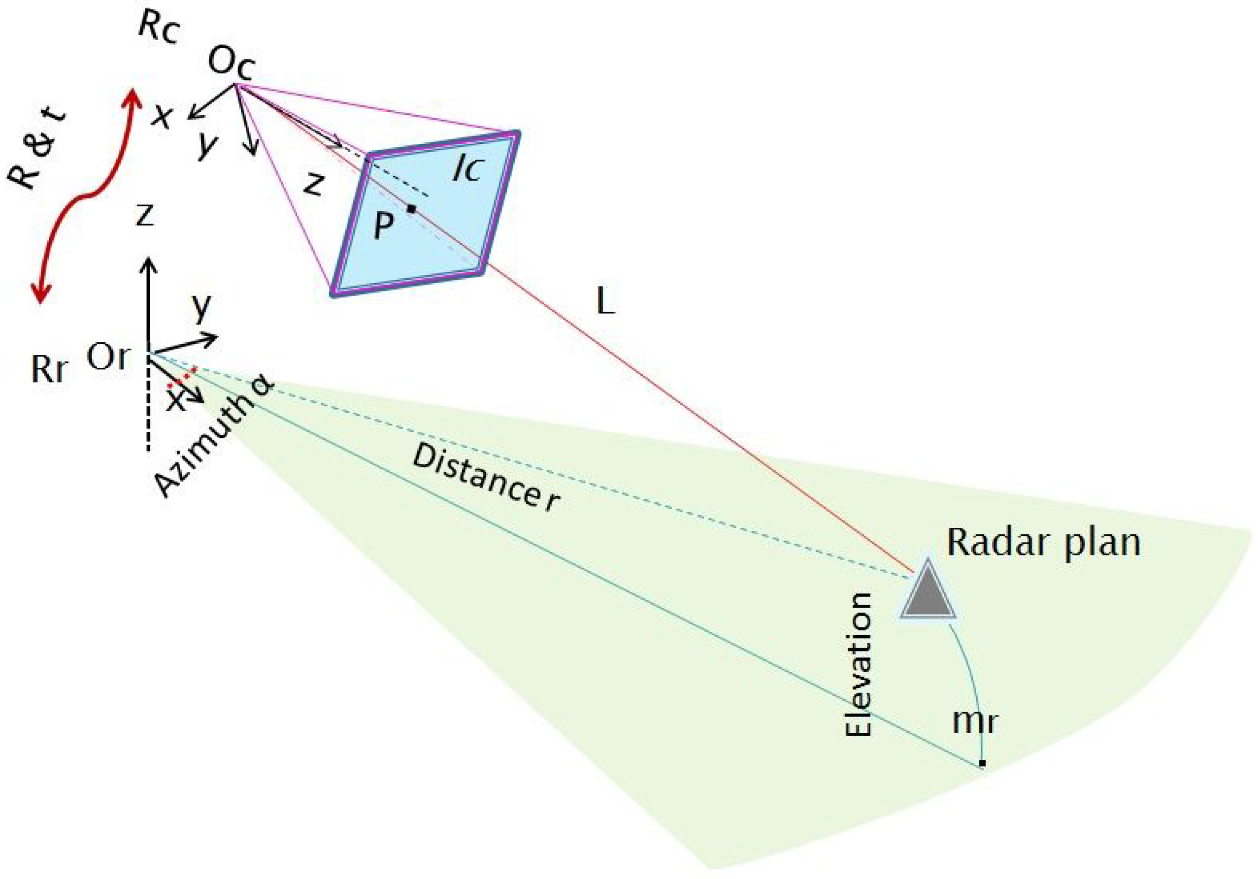
Figure 1.
The radar performs acquisitions over
per second thanks to its
step rotating antenna. It generates a panoramic image each second, where detected targets are localized in 2D polar coordinates. The radar locates a target in range and angle. The radar to target distance measurement is based on the FMCW principle [
33]. It can be shown that the frequency difference (called the beat frequency) between the transmitted signal and the signal received from a target is proportional to the sought distance. The reflected signal has a different frequency because of the continuous variation of the transmitted signal around a fixed reference frequency. The lateral resolution of the radar is about
(see
Table 1). The radar suffers from a low vertical resolution because of the wide angular aperture of the beam (
). The received signal echoes within this angular aperture (
), which is then integrated to form a single target.
Figure 1.
Sensors system geometry: and are the camera and radar frames, respectively. Polar coordinates of the target are provided by the radar data, but not the elevation angle. The light ray L and the projected point p in the image are shown together with the horizontal radar plane.
Figure 1.
Sensors system geometry: and are the camera and radar frames, respectively. Polar coordinates of the target are provided by the radar data, but not the elevation angle. The light ray L and the projected point p in the image are shown together with the horizontal radar plane.
Therefore, a 3D point detected by the radar is projected onto the horizontal plane passing through the center of the antenna first lobe of the radar, following a circular projection. Therefore, the real depth and azimuth of a detected target are provided without any altitude information. The projected point is denoted , where α and r are the polar coordinates of the point in the 3D space.
The camera performs a perspective projection relative to its optical center, consisting of two transformations: the first transformation projects a 3D point
into
(in a homogeneous coordinates system) in the image plane
, and it is written as follows:
where
w is a scale factor representing the depth of
relative to the camera.
K is the matrix of intrinsic parameters, assumed to be known, since the camera is calibrated using the MATLAB toolbox of [
34]. The vertical and horizontal dimensions of a pixel of the optical photosensitive sensor are denoted
and
, so
and
. The principal point
is the intersection of the optical axis and the image plane.
and
are the vertical and horizontal scaling factors, respectively expressed in pixel/mm, assuming that the photosensitive cells of a camera are not perfectly square. Additionally,
s is the skew parameter assuming that the two directions of the image sensors are not perfectly orthogonal. With recent devices, this parameter is very negligible in practice. The resulting camera matrix obtained is:
Secondly, a 3D transformation (rotation
R and translation
t) maps any point
from the camera frame
to a point
in the radar frame
, such as:
with
A the extrinsic matrix parameters:
Replacing
in Equation (1) by the formula in Equation (3) provides the final transformation mapping of the 3D to 2D points as follows:
3. Three-Dimensional Reconstruction
Because of the geometrical projection performed by the sensors, part of the information is lost during acquisition. The 3D reconstruction of a scene is then the compensation of the missing data from two-dimensional acquisitions. The 3D reconstruction of a large-scale environment is a challenging topic. For these reasons, the proposal of a simple, robust and fast algorithm dedicated to complete such an objective represents a major interest for several applications. Our goal is to prove the concept of using radar, which is underrated for 3D reconstruction, and to build a simple 3D sensor that is easy to use by a non-expert operator, which provides textured elevation maps, as illustrated in
Figure 2.
In order to achieve the 3D reconstruction, preliminary steps must be carried out. These steps are illustrated in
Figure 3: the data acquisition should be done simultaneously by each sensor having an overlapping field of view.
The acquisitions are synchronized using GPS data. The calibration step consists of determining the transformation mapping target coordinates from one sensor frame to another.
The feature extraction and matching between the data provided by these two sensors are essential, yet difficult process, since the data are inherently different; thus, they cannot be easily compared or matched. For the current stage, further works are in progress in order to automate this step.
Figure 2.
An illustration of the elevation map generation exploiting radar and vision complementarity.
Figure 2.
An illustration of the elevation map generation exploiting radar and vision complementarity.
Figure 3.
In order to achieve the 3D reconstruction, three preliminary steps must be carried out: simultaneous data acquisition by the sensors, the estimation of the transformation between the sensor frames and the extraction and matching of features from the camera image and the radar panoramic. (a) Data acquisition; (b) System calibration; (c) Features extraction and matching.
In order to recover the third dimension, we proceed as follows: a 3D point
Q detected by the camera and by the radar belong, in fact, to the light ray
L passing through the optical center of the camera, and at the same time, this belongs to a sphere
C, centered on the radar’s antenna center, as shown in
Figure 3. Therefore, its 3D coordinates are obtained by estimating the coordinate of the intersection point between the sphere
C and the straight
L.
The equation of the sphere is written as follows:
where
and
r are the sphere center and radius, respectively, in the camera coordinate frame. Additionally, the light ray equation is Equation (1), with
w the unknown parameter:
Our method consists of three steps: First, the scale factor
w is to be determined. From Equation (7),
x,
y and
z can be written as a function of
w:
,
and
. Replacing
x,
y and
z in Equation (6) thereby leads to a quadratic equation in
w:
Figure 4.
The 3D reconstructed point Q is the intersection of light ray L and the sphere C at α. is the projected 2D point on the horizontal radar plane, and is the vertical plane of the target at α.
Figure 4.
The 3D reconstructed point Q is the intersection of light ray L and the sphere C at α. is the projected 2D point on the horizontal radar plane, and is the vertical plane of the target at α.
Since we are working in a large-scale environment, the targets are usually too far compared to the baseline
B (the distance between the radar and camera frames). Then, the camera is always inside the sphere
C, so theoretically, two solutions for the quadratic Equation (9) exist as illustrated in
Figure 4,
w and
. From these solutions, two points
and
relative to the vision sensor frame are deduced from Equation (7). Secondly, their coordinates in the radar frame should be computed from Equation (3):
Finally, the azimuth angles of these 3D points are computed. Thereby, the correct solution is selected by comparing the computed azimuth angles and the one measured by the radar. The calibration step is then requisite in order to determine the transformation matrix A and the radar center .
4. System Calibration
The calibration is an important factor affecting the reconstruction accuracy. Hence, it is required to develop an accurate calibration method and with a rather simple implementation.
4.1. Related Work
The closest work on camera-radar system calibration is the work of
S. Sugimoto
et al. [
31]. The radar acquisitions are considered to be coplanar, since it performs a planar projection on its horizontal plane. Therefore, the transformation
A is a homography
H between image and radar planes, without going through the calculation of the rotation and translation matrices. For
(horizontal plane), these pairs are related as shown in Equation (11):
H is a homography matrix, relating camera and radar planes.
In spite of its theoretical simplicity, this method is hard to implement. Indeed, while the canonical target is being continuously moved up and down by a mechanical system, it should be simultaneously acquired by the radar and camera. Then, pairs of matches (four pairs at least), corresponding to the exact intersection of the target with the horizontal plane of the radar, are extracted. Moreover, due to the sampling frequency, the exact positions are determined from the maximum of the intensity reflected by the target using bilinear interpolation of the measurement samples along the vertical trajectory of each target.
4.2. The Proposed Calibration Method
Our goal is to determine the rotation and the translation between the frames of the sensors. For an azimuth angle
α, we have
, the normal to the plane
. Since
is a vertical plane passing by
, it has the following equation:
The equation of the sphere
C centered on
becomes:
From Equation (5), the 3D point
is expressed as a function of
,
w and
A as follows:
From Equation (14),
X,
Y and
Z can be expressed in terms of unknown
A and
w:
For
n matches, system
is obtained, with
and
ϵ the residuals:
The equations are expressed with respect to a parameter vector ; γ are the three rotational angles relative to x, y and z. The system is underdetermined, and many solutions exist, hence the need to add more geometric constraints.
4.3. Inter-Distance Constraint
In order to calculate the scale factor
w for each target, we propose to use the theorem of Al-Kashi [
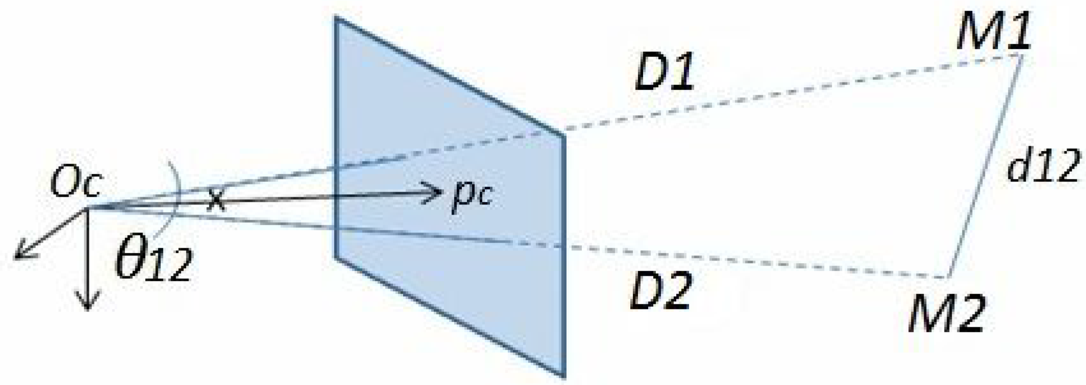
35]. This theorem is known as the “law of cosines” that generalizes the Pythagorean theorem of an unspecified triangle. The latter, applied to the triangle formed by two 3D points
,
with
, as illustrated in
Figure 5, gives the following equations:
where:
Figure 5.
The triangle formed by , (3D points in the camera frame) and is shown. is the Euclidean distance between and that is supposed to be known, and , are their depths relative to .
Figure 5.
The triangle formed by , (3D points in the camera frame) and is shown. is the Euclidean distance between and that is supposed to be known, and , are their depths relative to .
The only constraint for the proposed method is the
a priori knowledge of distances between the targets used for calibration. For
n matches with
,
is the depth of the point relative to
, and it is related to the scale factor
and the angle
formed between the principle point
and pixel
by the formula:
with:
is the known distance between points, and
is the angle between two rays lining up the 3D points with
(see
Figure 5). The cosine of
is calculated from corresponding pixels in the image and intrinsic matrix K in this manner:
Since we have six degrees of freedom (DOF), three for the rotation angles and three for the translation, relative to
x,
y and
z, we need at least six points. With six 3D points, we have 15 inter-distances, so we obtain a system
of 15 equations in terms of
, and
are the residuals:
The system is solved by the algorithm of Levenberg–Marquardt, based on non-linear least squares optimization of the sum of squared residuals
, in order to determine the approximate solution as shown hereafter:
4.4. Relaxation of the Inter-Distance Constraint
For further simplification of the implementation process, we tend to relax the
a priori inter-distance constraint, which could also be an additional source of error. In this context, geometrical equations should be added to the system in the optimization process. We propose to do so by moving the system of sensors, while keeping the captured scene fixed (see
Figure 6). This allows for multiple acquisitions of the scene from different points of view and provides additional equations.
Figure 6.
The displacement of the system around a fixed scene gives more geometric equations. An illustration of this process is shown. The matrix represent the transformation between one position and another.
Figure 6.
The displacement of the system around a fixed scene gives more geometric equations. An illustration of this process is shown. The matrix represent the transformation between one position and another.
Following this change of the point of view of the acquisitions, an additional transformation matrix , corresponding to a displacement k of the system, is to be determined. A 3D point in the radar frame is then expressed as a function of unknown A, and w as follows:
Additionally, for
, we have:
With i representing the number of 3D points, and is the corresponding pixel.
Thus,
,
and
can be written as follows:
Then, the following system
of two additional equations is obtained, for each point
i from a displacement
k:
For and , we have a total of 14 unknowns and equations, so a total of 32 equations; thus, the system is overdetermined. The parameter vector would be then: .
The resulting cost function is then optimized using the Levenberg–Marquardt least square optimization algorithm, in order to determine the unknowns:
The number of targets i depends on the number of displacements k, such that the more the system is moved, the fewer the targets that will be needed.
5. Uncertainty Analysis
In order to study the effect of several parameters on the accuracy of the proposed method, simulations on synthetic data were carried out using MATLAB. Sets of 3D points are randomly generated following a uniform random distribution within a cubic work space in front of the camera-radar system.
The projected pixel and the polar coordinates of each 3D point are computed using the pinhole model of the camera and the geometric model of the radar sensor, as explained in
Section 2.
First, the calibration and reconstruction algorithms were tested with exact data input, and the obtained errors are around 10 on translation, 10 on rotation and around 10 for the reconstruction method. Afterwards, the simulations were extended emulating realistic cases in order to test the efficiency and the robustness of the methods with respect to several parameters, such as the number of matches, the noise level, the baseline length and the elevation of the target. Therefore, synthetic data are disrupted by uniformly-distributed random noise.
Both calibration methods were tested, and the simulations results are discussed and compared in this section. For the first step, we added noise corresponding to ±2 pixels, ±
for the azimuth angle and ±2 cm for the distance. The number of matched points used for the calibration process is increased by a step of onefrom five to 30 points, and the calibration, using the two constraints, respectively, is done in order to analyze the convergence of the algorithms. The mean and standard deviation of the RMS error upon six specimens are shown in
Figure 7a,b.
It is noticeable that the shapes of the error curve, for both translation and rotation, are similar regardless of the method of calibration used. As might be expected, the errors decrease starting from six matches for both calibration methods, and then, they remain nearly stable. This is due to the non-linear problem that converges more precisely to the correct solution when the noisy equation system is over-determined.
It can be also noticed that the results of the second method in
Figure 7b, show more accurate behavior with increasing number of points at the same noise level; this is due to a larger number of equations used for this method and, therefore, a better convergence.
Secondly, in order to test the accuracy of the calibration, linearly increasing the noise level is applied to the input data starting from Level 1, corresponding to ±0.5 pixels, ±
for the azimuth angle and ±5 cm for the distance, up to Level 25, corresponding to ±5 pixels, ±
for the azimuth angle and ±50 cm for the distance. Error graphs are shown in
Figure 8a,b.
Figure 7.
Calibration error with respect to the number of points. Left column: translation error in meters; Right column: rotation error in radians. The graphs show the mean and the standard deviation of RMSE upon six iterations. The number of matches is increased by a step of one from three to 30, and the noise level is: ±2 p, ± for α, ± 2 cm for r. (a) First calibration method; (b) Second calibration method.
Figure 8.
Calibration error with respect to the noise level. Left: translation error in meters; Right: rotation error in radians. The graphs show the mean and the standard deviation of RMSE upon six reiterations with 10 matches used. (a) First calibration method; (b) Second calibration method.
Figure 8.
Calibration error with respect to the noise level. Left: translation error in meters; Right: rotation error in radians. The graphs show the mean and the standard deviation of RMSE upon six reiterations with 10 matches used. (a) First calibration method; (b) Second calibration method.
The number of matches used for the calibration process is 10. The mean and the standard deviation of the RMS error upon six specimens are also shown for the translation and rotation results. It should be noticed that the effects of the increasing noise on the rotation and translation increase the errors: non-linear algorithms are affected by noise, and yet, our algorithms show an acceptable behavior in the presence of noisy data. The results of the second method in
Figure 8b show a smaller increase compared to the first curves in
Figure 8a with increasing noise level.
The accuracy of the reconstruction method is similarly tested with respect to the same noise levels, and the resulting error graph is shown in the
Figure 9.
Figure 9.
Reconstruction error with respect to the noise level. The error is in meters relative to the point depths r. The mean and standard deviation of the RMSE, over 50 reconstructed points, are shown.
Figure 9.
Reconstruction error with respect to the noise level. The error is in meters relative to the point depths r. The mean and standard deviation of the RMSE, over 50 reconstructed points, are shown.
The graph in
Figure 9 shows the mean and standard deviation of the RMSE upon 50 reconstructed points for each level. Despite the slight increase of the error with increasing noise level, it is quite clear that the method is very robust in the presence of noise. For example, for the 25th level corresponding to ±5 pixels, ±
for the azimuth angle and ±50 cm for the depth, the error mean is about
m, which is a quite good result.
The influence of the baseline between the sensor centers, on the reconstruction methods, is also studied with simulated noisy data. The input data are this time disrupted with a fixed noise level corresponding to ±2 pixels, ±
and ±2 cm. The baseline width is increased from 0 cm up to 12 m in length. The resulting graph is shown in
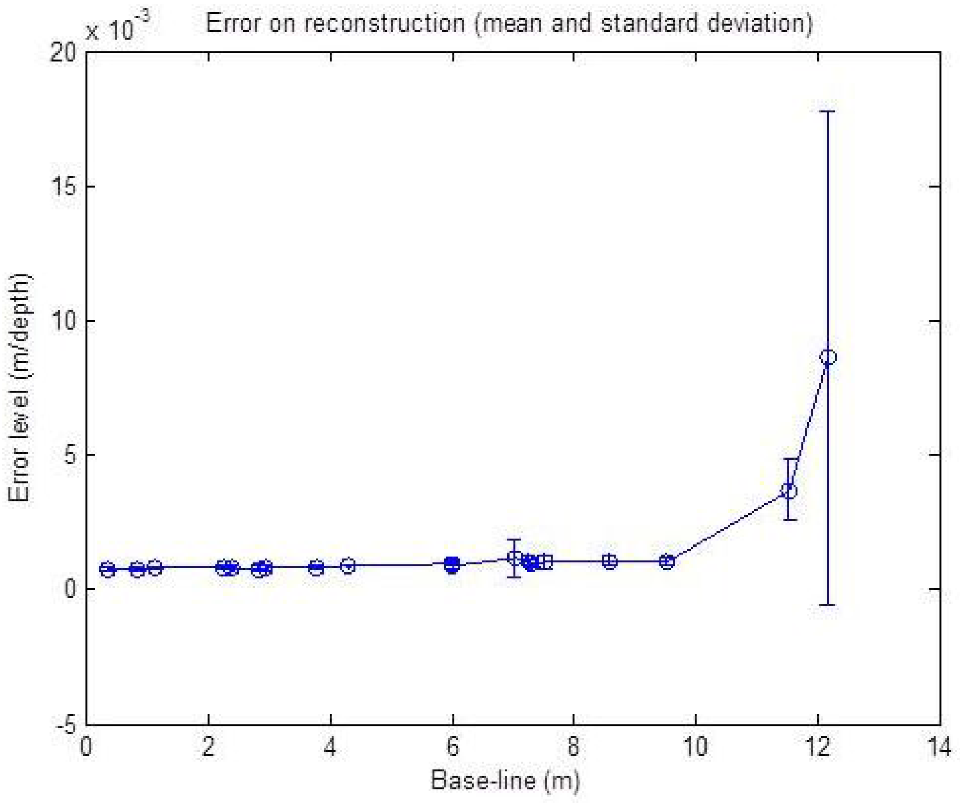
Figure 10. The graph shows the RMSE mean and standard deviation over 50 reconstructed points for each level.
Figure 10.
Reconstruction error with respect to the baseline with a noise level corresponding to ±2 p, ± for α and ±2 cm for r. The error is in meters relative to the point depths (r). The mean and standard deviation over 50 reconstructed points are shown.
Figure 10.
Reconstruction error with respect to the baseline with a noise level corresponding to ±2 p, ± for α and ±2 cm for r. The error is in meters relative to the point depths (r). The mean and standard deviation over 50 reconstructed points are shown.
The result of this simulation shows a nearly stable error level for the baseline under a 10 m width. Starting from 10 m, we can see a slight increase of the error level with respect to the increasing width. This is due to the geometric constraint, as shown in
Figure 11: in the presence of noise, for two different baseline widths, the intersection of the uncertainty regions of each sensor is not affected by the baseline width.
Figure 11.
Illustration of the baseline effect on the reconstruction error. (a) Intersection uncertainty using a narrow baseline; (b) Intersection uncertainty using a wide baseline.
Figure 11.
Illustration of the baseline effect on the reconstruction error. (a) Intersection uncertainty using a narrow baseline; (b) Intersection uncertainty using a wide baseline.
However, a very slight increase is observed when the baseline width is greater than the depth of the target, as shown in
Figure 12. However, this is not considered an issue for large-scale scenes and can be ignored, since the camera is often closer to the radar than the surrounding targets.
Figure 12.
The effect of the baseline is illustrated. The intersection of the uncertainty regions of each sensor projection is also shown. (a) Short baseline; (b) Wide baseline; (c) Wide baseline.
Figure 12.
The effect of the baseline is illustrated. The intersection of the uncertainty regions of each sensor projection is also shown. (a) Short baseline; (b) Wide baseline; (c) Wide baseline.
According to this study on the baseline parameter, we can consider from the above results that our reconstruction method does not require a constrained baseline width, unlike the vision-based methods, where the baseline width has a strong especial affect on the results for large-scale scenes. Indeed, in vision-based approaches, distant targets require a longer baseline in order to reduce the range uncertainty of the 3D reconstruction, as illustrated in
Figure 13d. Only having further afield points of view leads to a decreased common area between the two acquisitions, thereby affecting the complexity of the image registrations. The error on the pixel in the image camera is derived from the camera projection error and the extraction uncertainty of the targets. The error on the radar data is the uncertainty for the azimuth angle of
, corresponding to
, and for the depth of 0.02 m. In the ideal case, the reconstruction is done by calculating the intersection between a straight and a sphere, as illustrated in the
Figure 13a. However, introducing the uncertainty of each sensor to the geometric model, the reconstruction error is then the intersection of the cone corresponding to the camera uncertainty zone and the inter-sphere region corresponding to the radar uncertainty zone (see
Figure 13b). The intersection zone between the sphere and the cone can be approximated to an ellipse. Therefore, the error corresponds to a truncatedoblique cone, as illustrated in
Figure 13c, having a volume
, where
and
correspond to the major and minor axes of the base ellipse and top ellipse, respectively. The height of the truncatedcone is equal to the difference between the maximum and minimum depth in the uncertainty zone.
Figure 13.
The intersection of the uncertainty regions of each sensor’s projection: (a) the ideal case of the geometric reconstruction; (b) introducing uncertainty regions of each sensor to the geometric model; (c) the error intersection region; (d) uncertainity intersection region in respect to the baseline for the stereo reconstruction method.
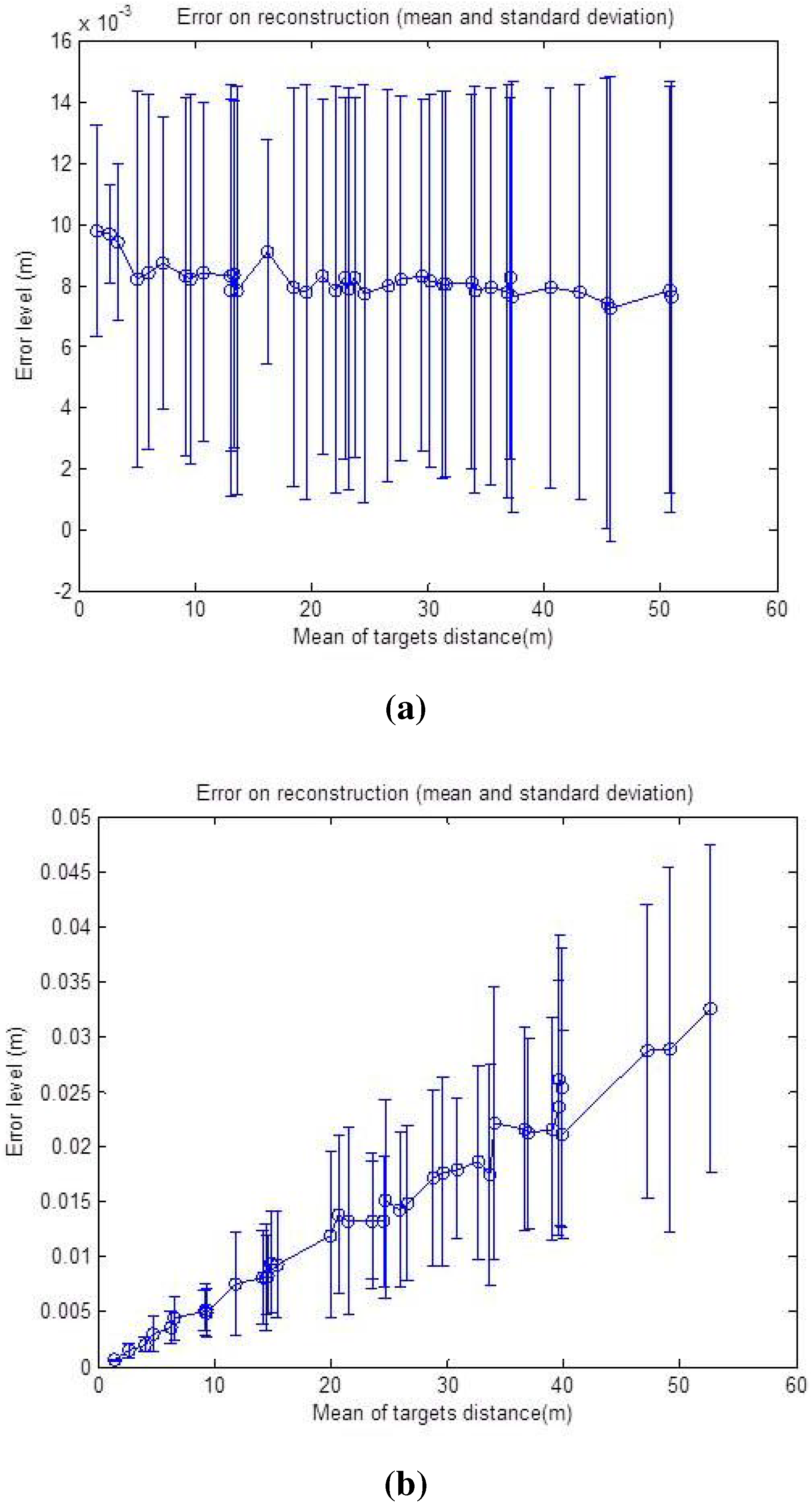
The same noise level is added on simulated data in order to study the effects of targets depths on the error level for the reconstruction algorithm. The resulting graphs are shown in
Figure 14 and
Figure 15, respectively.
First, the noise is added just to the radar data (zero for the pixel, ±
for
α and ±2 cm for
r) and then to the data from the camera (±2 for the pixel,
for
α and 0 cm for
r), as the uncertainty zone changes differently for the two sensors with the increasing distance of the targets. One can remark from the graph in
Figure 14a that the reconstruction error is oscillating around 1 cm, and it is almost stable compared to a growing target depth. This is explained by the fact that the precision of the radar measurement is stable with respect to the distance. The geometric interpretation is illustrated in
Figure 15a, where the error of the reconstruction is only depending on the error of the depth of the target, which is independent of distance. The azimuth provided by the radar is not taken into account in the reconstruction Equation (9). On the other hand, the graph in
Figure 14b shows that the uncertainty zone of the camera increases with distance and, thus, increases the reconstruction error, as can be seen in
Figure 15b.
Thereby, the effect of this parameter on the reconstruction method is shown in
Figure 16. As we can see, the graph shows a rising error level caused by the camera rising uncertainty zone, but the minimum error level at the beginning of the curve is this time affected by the noise on the depth
r. This is illustrated in
Figure 16; for a shallow depth, the uncertainty zone of the camera is smaller than that of the radar, and then, it increases with distance.
Figure 14.
Reconstruction error with respect to the mean depth of the targets. The error is in meters. The mean and standard deviation of the RMSE, over 50 reconstructed points, are shown. (a) Noise added corresponding to 0 p, ± for α and ±2cm for r; (b) Noise added corresponding to ±2 p, for α and 0 cm for r.
Figure 15.
Illustration of the baseline effect on the reconstruction error. (a) Noise added only to radar data; (b) Noise added only to camera data; (c) Noise added to both camera and radar data.
Figure 15.
Illustration of the baseline effect on the reconstruction error. (a) Noise added only to radar data; (b) Noise added only to camera data; (c) Noise added to both camera and radar data.
Figure 16.
Reconstruction error with respect to the mean depth of the targets with a noise level corresponding to ±2 p, ± for α and ±2 cm for r. The error is in meters. The mean and standard deviation of the RMSE, over 50 reconstructed points, are shown.
Figure 16.
Reconstruction error with respect to the mean depth of the targets with a noise level corresponding to ±2 p, ± for α and ±2 cm for r. The error is in meters. The mean and standard deviation of the RMSE, over 50 reconstructed points, are shown.
6. Experimental Results
In order to validate the theory of the proposed methods, experiments on real data were carried out. The radar and the camera were mounted in a fixed configuration on the top of a vehicle, in front of the scene (for the current stage, the radar antenna rotates
, but the camera is stable). The radar is called K2Pi and has been developed by Irstea Institute. The optic sensor used is uEye by IDS (Imaging Development Systems). The camera and radar characteristics are listed in
Table 1. A GPS mounted on the vehicle has been used for the synchronization of the data acquisition carried out by these two sensors. The system is shown in
Figure 17. The baseline between the sensors is about 60 cm.
Table 1.
Camera and radar characteristics.
Table 1.
Camera and radar characteristics.
| Camera Characteristics |
|---|
| Sensor technology | CMOS |
| Sensor size | mm |
| Pixel size | mm |
| Resolution in pixel | |
| Focal distance | 8 mm |
| Viewing angle | |
| Radar Characteristics |
| Carrier frequency | 24 GHz |
| Antenna gain | 20 dB |
| Range | 3 to 100 m |
| Angular resolution | |
| Distance resolution | 1 m |
| Distance precision | 0.02 m |
| Viewing angle | |
Figure 17.
Radar and camera system. The image to the right presents the zoom in of the sensors system (the radar to the right and the camera to the left).
Figure 17.
Radar and camera system. The image to the right presents the zoom in of the sensors system (the radar to the right and the camera to the left).
At the beginning, the system should be calibrated; we placed eight canonical targets in front of the sensor system. Metallic canonical targets (
Figure 18) are highly reflective regardless of their position relative to the radar and with a small cross-section. The depth of the targets is chosen to be slightly close: between 6 m and 14 m for the first calibration method and between 10 m and 17 m for the second calibration method. The sensor system is placed in a manner that will enable clear acquisitions of the targets by the camera and the radar simultaneously (thus, there is a limited depth), and it should also be compatible with the context of the practical usage of the system. For the second calibration method, the system was moved several times in order to capture the scene from different points of view. This is in order to facilitate feature extraction from the images. The features extracted for the calibration experiments are the target centers. Centers are matched manually, and
Figure 19 shows the corresponding pixels and radar targets extracted in the image of the camera and the panoramic image.
Figure 18.
Center detection of targets in both the camera image and radar panoramic. (a) Radar target extraction; (b) Camera target extraction.
Figure 18.
Center detection of targets in both the camera image and radar panoramic. (a) Radar target extraction; (b) Camera target extraction.
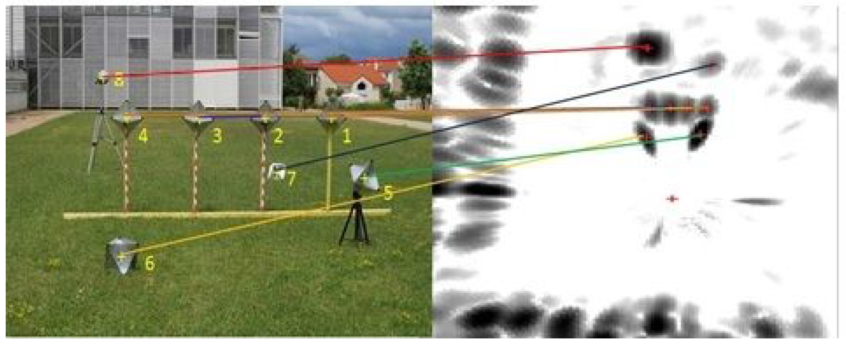
Figure 19.
An image and a panoramic of targets. The targets are numbered from 1 to 8: one Luneburg lens and seven trihedral corners. The yellow crosses indicate the centers of the targets. The variations of amplitude of the reflected signal are introduced by the nature and orientation of each target. Manually-extracted matches between the image and the PPI are shown.
The extraction of target centers in the radar images is done as follows:
First, the target centers are selected manually; then, Gaussian filtering is performed to be more specific. Gaussian estimation corresponding to the target is done, and the maximum position is then detected, as seen in
Figure 18a. Finally, we calculate the polar coordinates of the target. The center extraction method of the targets from the images is illustrated in
Figure 18b: the targets are painted in order to contrast the faces of the targets, so that their centers can be readily detected thanks to their special geometrical shape, using the Harris corner detector [
36]. Thus, the accuracy is assumed to be sub-pixel, as in classical camera calibration processes.
Figure 20.
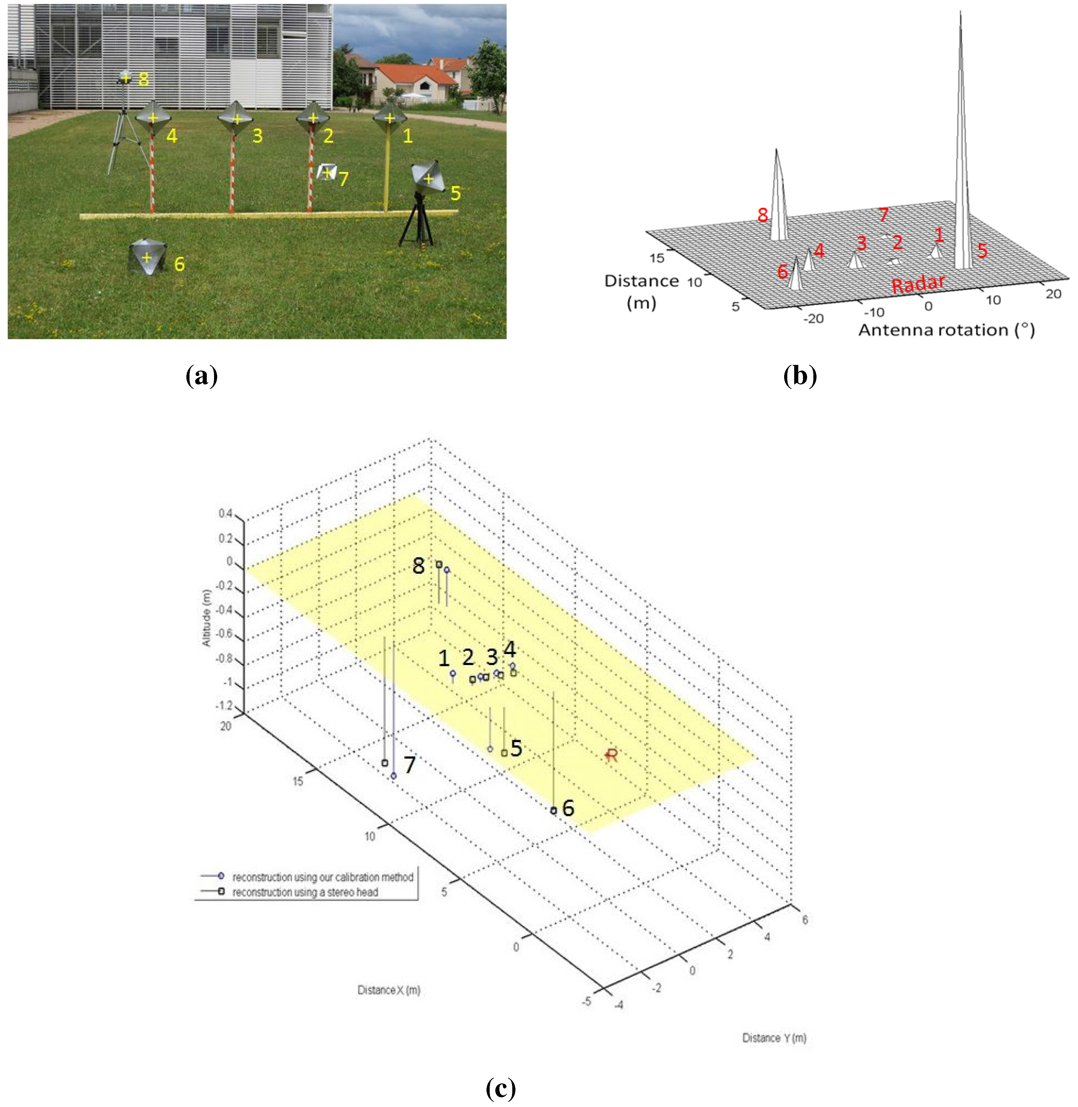
Reconstruction results using the inter-distance constraint for calibration. (a) Camera image of the eight canonical targets: one Luneburg lens and seven trihedral corners. The yellow crosses indicate the center of the targets; (b) Radar image with eight canonical targets; (c) The reconstruction results of both of our reconstruction methods (circular points) and the stereo head method as the ground truth (squared points). The radar position is indicated by the letter R.
Figure 20.
Reconstruction results using the inter-distance constraint for calibration. (a) Camera image of the eight canonical targets: one Luneburg lens and seven trihedral corners. The yellow crosses indicate the center of the targets; (b) Radar image with eight canonical targets; (c) The reconstruction results of both of our reconstruction methods (circular points) and the stereo head method as the ground truth (squared points). The radar position is indicated by the letter R.
In order to assess both results of the calibration method and to validate the reconstruction method, the eight targets were placed at different heights and depths. The reconstruction is obtained in the radar frame.
Figure 20 and
Table 2 represent the results of the reconstruction technique, using the method of
Section 4.3, and reconstruction results using a stereo head, used as the ground truth. The inter-distances between the targets centers are measured, and an image and panoramic of the eight targets in a random configuration are captured. The resulting 3D point clouds were registered using the ICP (iterative closest point) algorithm. The RMSE of the reconstruction method is about 0.63 m with a standard deviation of 0.15 m. The results show a realistic error for the 3D reconstruction of targets at a mean depth of 12 m.
Table 2.
Reconstruction results in m using the first calibration method.
Table 2.
Reconstruction results in m using the first calibration method.
| | Target Coordinates in Meters with the Stereo Head (Ground Truth) |
|---|
| X | 5.41 | 7.45 | 7.47 | 7.44 | 7.53 | 4.59 | 12.53 | 13.01 |
| Y | 1.32 | 1.45 | 0.70 | −0.03 | −0.78 | −0.68 | 2.24 | −1.03 |
| Z | −0.38 | 0.05 | 0.02 | −0.01 | −0.06 | −0.92 | −1.05 | 0.33 |
| | Targets Coordinates in Meters with the Developed Method |
| X | 5.50 | 7.55 | 7.53 | 7.46 | 7.51 | 4.57 | 12.64 | 12.98 |
| Y | 0.83 | 0.86 | 0.11 | −0.62 | −1.37 | −1.12 | 1.40 | −1.89 |
| Z | −0.35 | 0.05 | 0.01 | −0.03 | −0.08 | −0.89 | −1.15 | 0.21 |
| | Error in Meters (Euclidean Distance) |
| | 0.49 | 0.60 | 0.59 | 0.59 | 0.59 | 0.44 | 0.85 | 0.87 |
| | Error mean in meters = 0.63 |
| | Error standard deviation in meters = 0.15 |
Table 3.
Reconstruction results in m using the second calibration method.
Table 3.
Reconstruction results in m using the second calibration method.
| | Targets Coordinates in Meters with the Stereo Head (Ground Truth) |
|---|
| X | 14.21 | 14.40 | 14.58 | 16.85 | 17.91 | 18.55 | 20.04 | 21.70 |
| Y | −3.08 | −0.02 | 2.05 | −4.53 | 0.53 | 3.88 | −3.21 | −0.15 |
| Z | −0.19 | −0.18 | −0.17 | −1.10 | 0.28 | −0.90 | 0.98 | −0.61 |
| | Targets Coordinates in Meters with the Developed Method |
| X | 12.57 | 12.56 | 12.53 | 15.20 | 15.94 | 16.59 | 18,56 | 19,52 |
| Y | −3.09 | 0.03 | 2.09 | −4.59 | 0.55 | 3.96 | −3,20 | −0,058 |
| Z | 0.09 | 0.14 | 0.19 | −1.03 | 0.35 | −0.85 | 0,88 | −0,79 |
| | Error in Meters (Euclidean Distance) |
| | 0.05 | 0.04 | 0.06 | 0.05 | 0.05 | 0.03 | 0.08 | 0.11 |
| | Error- mean in meters = 0.058 |
| | Error- standard deviation in meters = 0.024 |
For the current stage, the system is not moved.
Figure 21 and
Table 3 represent the reconstruction results using the second calibration method. The results are also registered and compared to the ground truth stereo head reconstruction of the same scene. The RMSE mean is about 0.058 m with a standard deviation of 0.024 m on
and
Z.
Figure 21.
Top line: Camera images of the eight canonical targets. middle line: Radar images with eight canonical targets. The reconstruction results from both our reconstruction methods (circular points) and the stereo head method as the ground truth (squared points). The radar position is indicated by the letter R. (a) First position; (b) Second position; (c) Third position; (d) First position; (e) Second position; (f) Third position; (g) Reconstruction results.
Figure 22.
Results of a reconstructed urban scene using the camera/radar system and the second calibration method. The results are enhanced with texture mapping (this figure is clearer in color). (a) Camera image of an urban scene; (b) Segmented image (polygons are shown in red); (c) Part of the radar image of the same scene; (d) Segmented radar image; (e) Results of the reconstruction using Delaunay triangulation; (f) Enhanced results with texture; (g) Another view of the 3D results; (h) Another view of the 3D results.
Figure 23.
Results of a reconstructed urban scene using the camera/radar system, and the second calibration method. The results are enhanced with texture mapping (this figure is clearer in color). (a) Camera image of the an urban scene; (b) Segmented camera image; (c) Part of the radar image of the same scene; (d) Segmented radar image; (e) Results of the reconstruction using Delaunay triangulation; (f) Enhanced results with texture; (g) Another view of the 3D results; (h) Another view of the 3D results.
Figure 22 and
Figure 23 show the results of reconstructed urban scenes using our system. The camera/radar system is calibrated; the second calibration method is used for this experiment. Eight targets are captured by the system from three different points of view, as shown in
Figure 21. These results are interpreted qualitatively since no numerical ground truth results are available. The segmentation and matching of the data provided by the sensors are done interactively. Polygons are extracted from the images covering the targets of interest, and then their vertices are matched by pairs. This step is to be automated in future work. The matched points are then reconstructed and the polygons are plotted using the Delaunay triangulation algorithm, as shown in
Figure 22e and
Figure 23e. Finally, texture mapping is done in order to enhance the representation of the reconstructed map. In fact, the interest of this sensor fusion is shown in the example in
Figure 22, as the radar provides no information about the elevation of the bridge, this later being detected as a barrier. The elevation and vertical occupation of the bridge are extracted from the image of the camera. Therefore, this ambiguity is eliminated after the reconstruction process.


