
Optimal Sensor Selection for Classifying a Set of Ginsengs Using Metal-Oxide Sensors

Abstract
:1. Introduction
2. Experimental Section
2.1. Sample Preparation

| Sample No. | Ginseng Samples | Places of Production |
|---|---|---|
| 1 | Chinese red ginseng | Ji’an |
| 2 | Chinese red ginseng | Fusong |
| 3 | Korean red ginseng | Ji’an |
| 4 | Chinese white ginseng | Ji’an |
| 5 | Chinese white ginseng | Fusong |
| 6 | American ginseng | Fusong |
| 7 | American ginseng | USA |
| 8 | American ginseng | Canada |
| 9 | American ginseng | Tonghua |
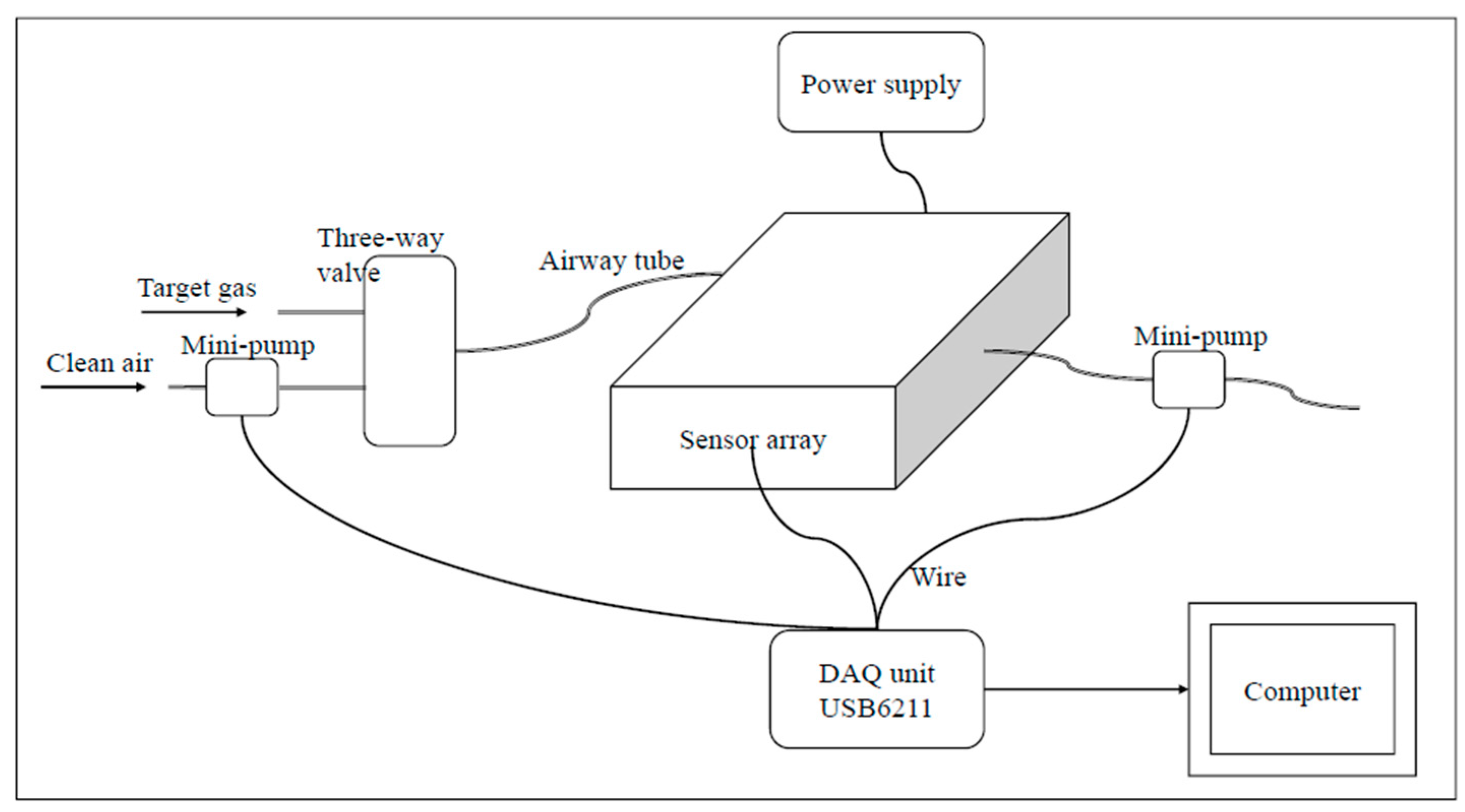
2.2. E-Nose Equipment

| No. | Sensor Type | Response Characteristics |
|---|---|---|
| 1 | TGS813 | Carbon monoxide, ethanol, methane, hydrogen, isobutane |
| 2 | TGS821 | Carbon monoxide, ethanol, methane, hydrogen |
| 3 | TGS822 | Carbon monoxide, ethanol, methane, acetone, n-Hexane, benzene, isobutane |
| 4 | TGS822 | Carbon monoxide, ethanol, methane, acetone, n-Hexane, benzene, isobutane |
| 5 | TGS826 | Ammonia, trimethyl amine |
| 6 | TGS832 | R-134a, R-12 and R-22, ethanol |
| 7 | TGS800 | Carbon monoxide, ethanol, methane, hydrogen, ammonia |
| 8 | TGS880 | Carbon monoxide, ethanol, methane, hydrogen, isobutane |
| 9 | TGS2600 | Carbon monoxide, hydrogen |
| 10 | TGS2602 | Hydrogen, ammonia ethanol, hydrogen sulfide, toluene |
| 11 | TGS2610 | Ethanol, hydrogen, methane, isobutane/Propane |
| 12 | TGS2611 | Ethanol, hydrogen, isobutane, methane |
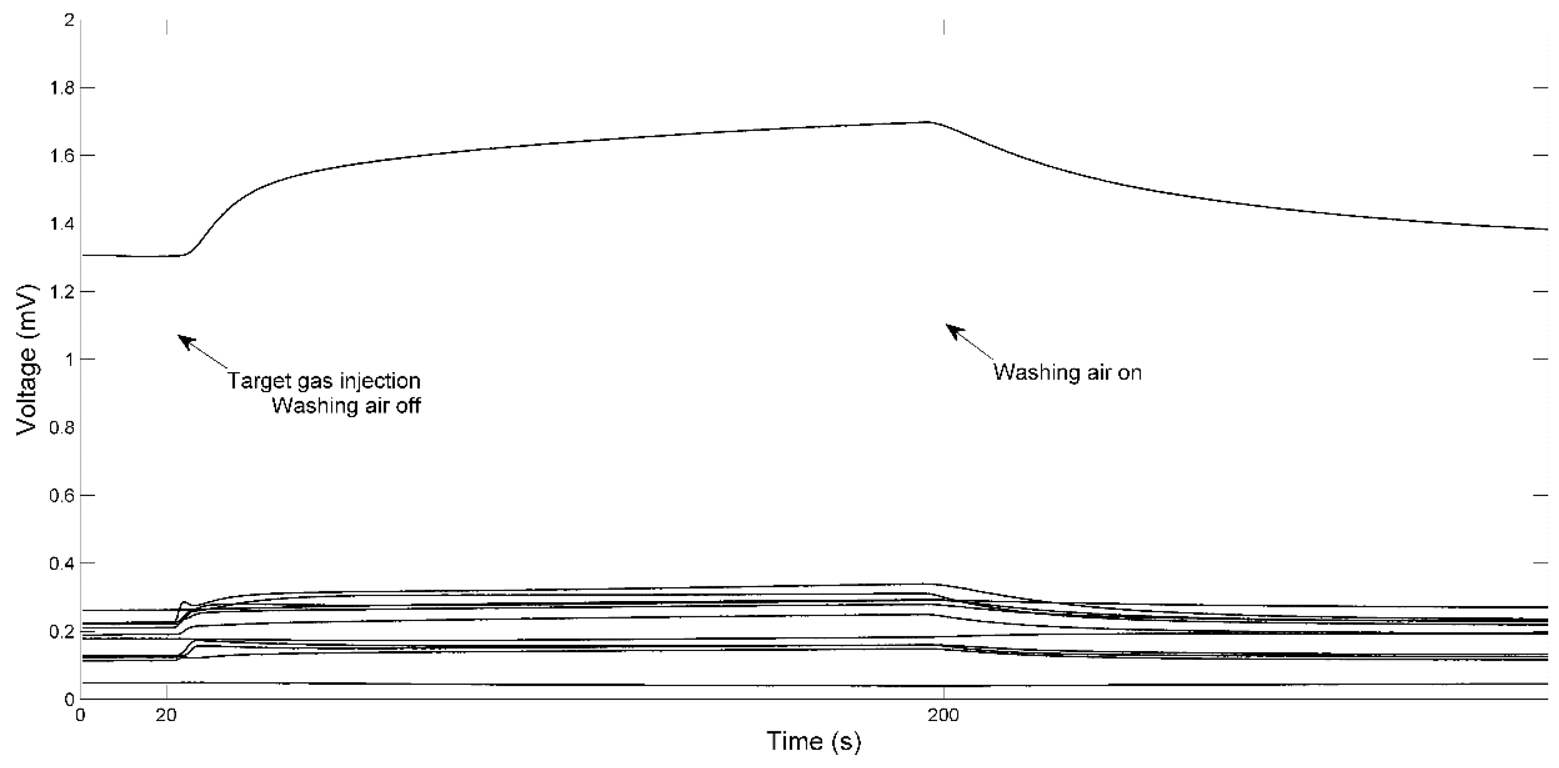
2.3. Measurement

2.4. Data processing
3. Results and Discussion
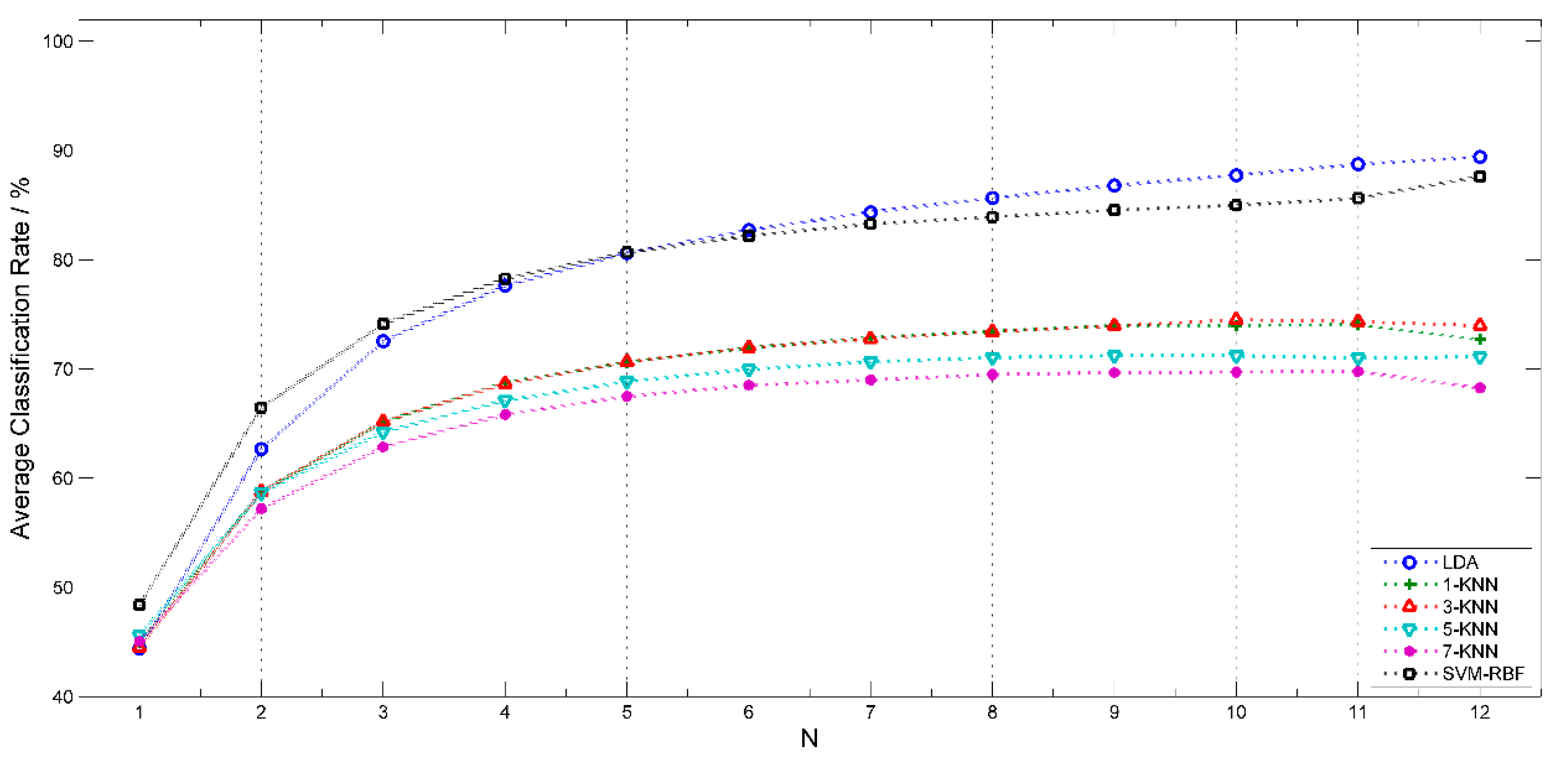
3.1. Comparison of Different Classification Algorithms

3.2. Classification Performance of All Potential Sensor Sets for All Potential Sample Sets

3.3. An Approach for Grading the Sensors for the Discrimination of a Certain Sample Set

| Step | Procedure | Sensors Estimation |
|---|---|---|
| 1 | Start | No. 3 +, 5 +, 10 +, 2 −, 8 −,11 −,12 − |
| 2 | Deleting No. 2, 8, 11, 12 sensors | No. 3 +, 10 +, 1 −, 7 − |
| 3 | Deleting No. 1, 7 sensors | No. 3 +, 10 +, 4 −, 6 − |
| 4 | Deleting No. 4, 6 sensors | No. 3 +, 10 + |
| 5 | Stop |
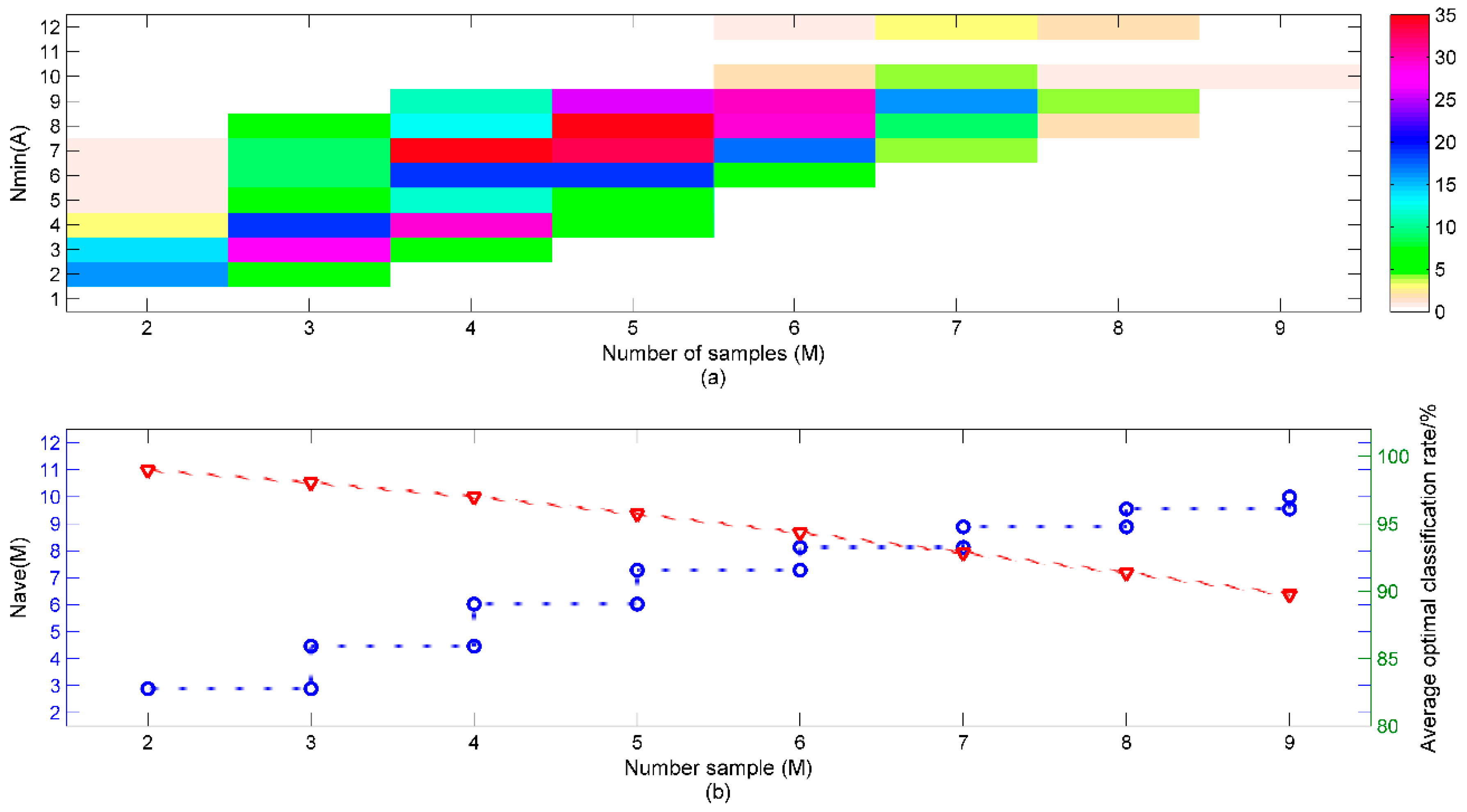
3.4. The Minimum Number of Sensors for All Potential Sample Sets

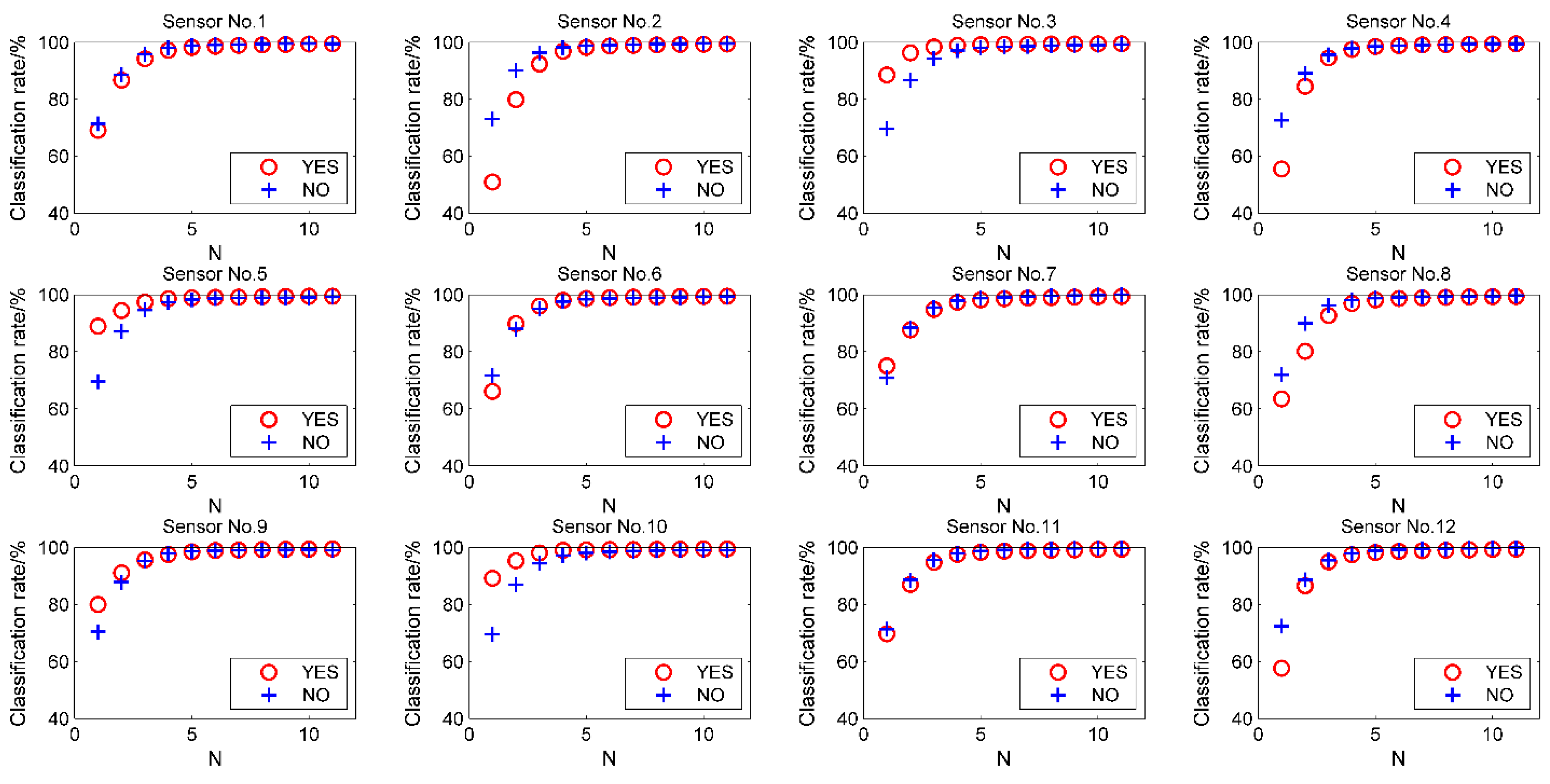
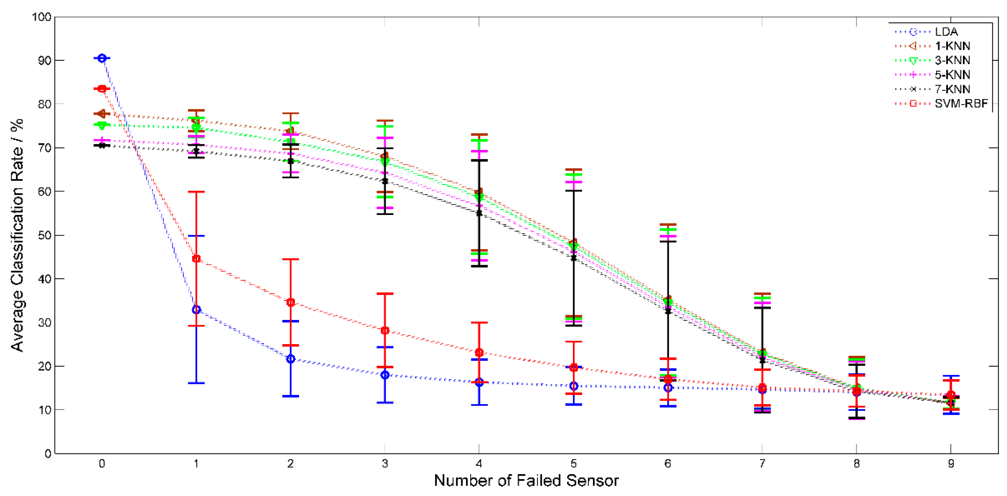
3.5. Impact on System Robustness by Sensor Failure

4. Conclusions
Acknowledgments
Author Contributions
Conflicts of Interest
References
- De Vito, S.; Piga, M.; Martinotto, L.; di Francia, G. CO, NO2 and NO(x) urban pollution monitoring with on-field calibrated electronic nose by automatic bayesian regularization. Sens. Actuators B Chem. 2009, 143, 182–191. [Google Scholar] [CrossRef]
- Zhang, L.; Tian, F.C.; Nie, H.; Dang, L.J.; Li, G.R.; Ye, Q.; Kadri, C. Classification of multiple indoor air contaminants by an electronic nose and a hybrid support vector machine. Sens. Actuators B Chem. 2012, 174, 114–125. [Google Scholar] [CrossRef]
- Musatov, V.Y.; Sysoev, V.V.; Sommer, M.; Kiselev, I. Assessment of meat freshness with a metal oxide sensor microarray electronic nose: A practical approach. Sens. Actuators B Chem. 2010, 144, 99–103. [Google Scholar] [CrossRef]
- Baldwin, E.A.; Bai, J.H.; Plotto, A.; Dea, S. Electronic noses and tongues: Applications for the food and pharmaceutical industries. Sensors 2011, 11, 4744–4766. [Google Scholar] [CrossRef] [PubMed]
- Ragazzo-Sanchez, J.A.; Chalier, P.; Chevalier-Lucia, D.; Calderon-Santoyo, M.; Ghommidh, C. Off-flavours detection in alcoholic beverages by electronic nose coupled to GC. Sens. Actuators B Chem. 2009, 140, 29–34. [Google Scholar] [CrossRef]
- Fu, J.; Huang, C.Q.; Xing, J.G.; Zheng, J.B. Pattern classification using an olfactory model with PCA feature selection in electronic noses: Study and application. Sensors 2012, 12, 2818–2830. [Google Scholar] [CrossRef] [PubMed]
- Schmekel, B.; Winquist, F.; Vikstrom, A. Analysis of breath samples for lung cancer survival. Anal. Chim. Acta 2014, 840, 82–86. [Google Scholar] [CrossRef] [PubMed]
- Montuschi, P.; Mores, N.; Trove, A.; Mondino, C.; Barnes, P.J. The electronic nose in respiratory medicine. Respiration 2013, 85, 72–84. [Google Scholar] [CrossRef] [PubMed]
- Chatterjee, S.; Castro, M.; Feller, J.F. An E-nose made of carbon nanotube-based quantum resistive sensors for the detection of eighteen polar/nonpolar VOC biomarkers of lung cancer. J. Mater. Chem. B 2013, 1, 4563–4575. [Google Scholar] [CrossRef]
- Hierlemann, A.; Gutierrez-Osuna, R. Higher-order chemical sensing. Chem. Rev. 2008, 108, 563–613. [Google Scholar] [CrossRef] [PubMed]
- Korotcenkov, G.; Cho, B.K. Instability of metal oxide-based conductometric gas sensors and approaches to stability improvement (short survey). Sens. Actuators B Chem. 2011, 156, 527–538. [Google Scholar] [CrossRef]
- Marco, S.; Gutierrez-Galvez, A. Signal and data processing for machine olfaction and chemical sensing: A review. IEEE Sens. J. 2012, 12, 3189–3214. [Google Scholar] [CrossRef]
- Zhang, L.; Tian, F.C. A new kernel discriminant analysis framework for electronic nose recognition. Anal. Chim. Acta 2014, 816, 8–17. [Google Scholar] [CrossRef] [PubMed]
- Gardner, J.W.; Boilot, P.; Hines, E.L. Enhancing electronic nose performance by sensor selection using a new integer-based genetic algorithm approach. Sens. Actuators B Chem. 2005, 106, 114–121. [Google Scholar] [CrossRef]
- Kaur, R.; Kumar, R.; Gulati, A.; Ghanshyam, C.; Kapur, P.; Bhondekar, A.P. Enhancing electronic nose performance: A novel feature selection approach using dynamic social impact theory and moving window time slicing for classification of Kangra orthodox black tea (Camellia sinensis (L.) O. Kuntze). Sens. Actuators B Chem. 2012, 166, 309–319. [Google Scholar] [CrossRef]
- Nowotny, T.; Berna, A.Z.; Binions, R.; Trowell, S. Optimal feature selection for classifying a large set of chemicals using metal oxide sensors. Sens. Actuators B Chem. 2013, 187, 471–480. [Google Scholar] [CrossRef]
- Phaisangittisagul, E.; Nagle, H.T.; Areekul, V. Intelligent method for sensor subset selection for machine olfaction. Sens. Actuators B Chem. 2010, 145, 507–515. [Google Scholar] [CrossRef]
- Zhang, L.; Tian, F.C.; Pei, G.S. A novel sensor selection using pattern recognition in electronic noses. Measurement 2014, 54, 31–39. [Google Scholar] [CrossRef]
- Phaisangittisagul, E.; Nagle, H.T. Sensor selection for machine olfaction based on transient feature extraction. IEEE Instrum. Meas. 2008, 57, 369–378. [Google Scholar] [CrossRef]
- Choi, S.I.; Jeong, G.M. A discriminant distance based composite vector selection method for odor classification. Sensors 2014, 14, 6938–6951. [Google Scholar] [CrossRef] [PubMed]
- Liu, Q.J.; Zhao, Z.M.; Li, Y.X.; Li, Y.Y. Feature selection based on sensitivity analysis of fuzzy isodata. Neurocomputing 2012, 85, 29–37. [Google Scholar] [CrossRef]
- Lee, S.K.; Kim, J.H.; Sohn, H.J.; Yang, J.W. Changes in aroma characteristics during the preparation of red ginseng estimated by electronic nose, sensory evaluation and gas chromatography/mass spectrometry. Sens. Actuators B Chem. 2005, 106, 7–12. [Google Scholar] [CrossRef]
- Cho, I.H.; Lee, H.J.; Kim, Y.S. Differences in the volatile compositions of ginseng species (Panax sp.). J. Agr. Food Chem. 2012, 60, 7616–7622. [Google Scholar] [CrossRef] [PubMed]
- Fonollosa, J.; Fernandez, L.; Huerta, R.; Gutierrez-Galvez, A.; Marco, S. Temperature optimization of metal oxide sensor arrays using mutual information. Sens. Actuators B Chem. 2013, 187, 331–339. [Google Scholar] [CrossRef]
- Green, G.C.; Chan, A.D.C.; Dan, H.H.; Lin, M. Using a metal oxide sensor (MOS)-based electronic nose for discrimination of bacteria based on individual colonies in suspension. Sens. Actuators B Chem. 2011, 152, 21–28. [Google Scholar] [CrossRef]
- Fonollosa, J.; Vergara, A.; Huerta, R. Algorithmic mitigation of sensor failure: Is sensor replacement really necessary? Sens. Actuators B Chem. 2013, 183, 211–221. [Google Scholar] [CrossRef]
- Chang, C.C.; Lin, C.J. LIBSVM: A library for support vector machines. ACM Trans. Intel. Syst. Technol. 2011, 2, 1–27. [Google Scholar] [CrossRef]
© 2015 by the authors; licensee MDPI, Basel, Switzerland. This article is an open access article distributed under the terms and conditions of the Creative Commons Attribution license (http://creativecommons.org/licenses/by/4.0/).
Share and Cite
Miao, J.; Zhang, T.; Wang, Y.; Li, G. Optimal Sensor Selection for Classifying a Set of Ginsengs Using Metal-Oxide Sensors. Sensors 2015, 15, 16027-16039. https://doi.org/10.3390/s150716027
Miao J, Zhang T, Wang Y, Li G. Optimal Sensor Selection for Classifying a Set of Ginsengs Using Metal-Oxide Sensors. Sensors. 2015; 15(7):16027-16039. https://doi.org/10.3390/s150716027
Chicago/Turabian StyleMiao, Jiacheng, Tinglin Zhang, You Wang, and Guang Li. 2015. "Optimal Sensor Selection for Classifying a Set of Ginsengs Using Metal-Oxide Sensors" Sensors 15, no. 7: 16027-16039. https://doi.org/10.3390/s150716027