
SNR Wall Effect Alleviation by Generalized Detector Employed in Cognitive Radio Networks

Abstract
:1. Introduction

2. System Model and GD Test Statistics
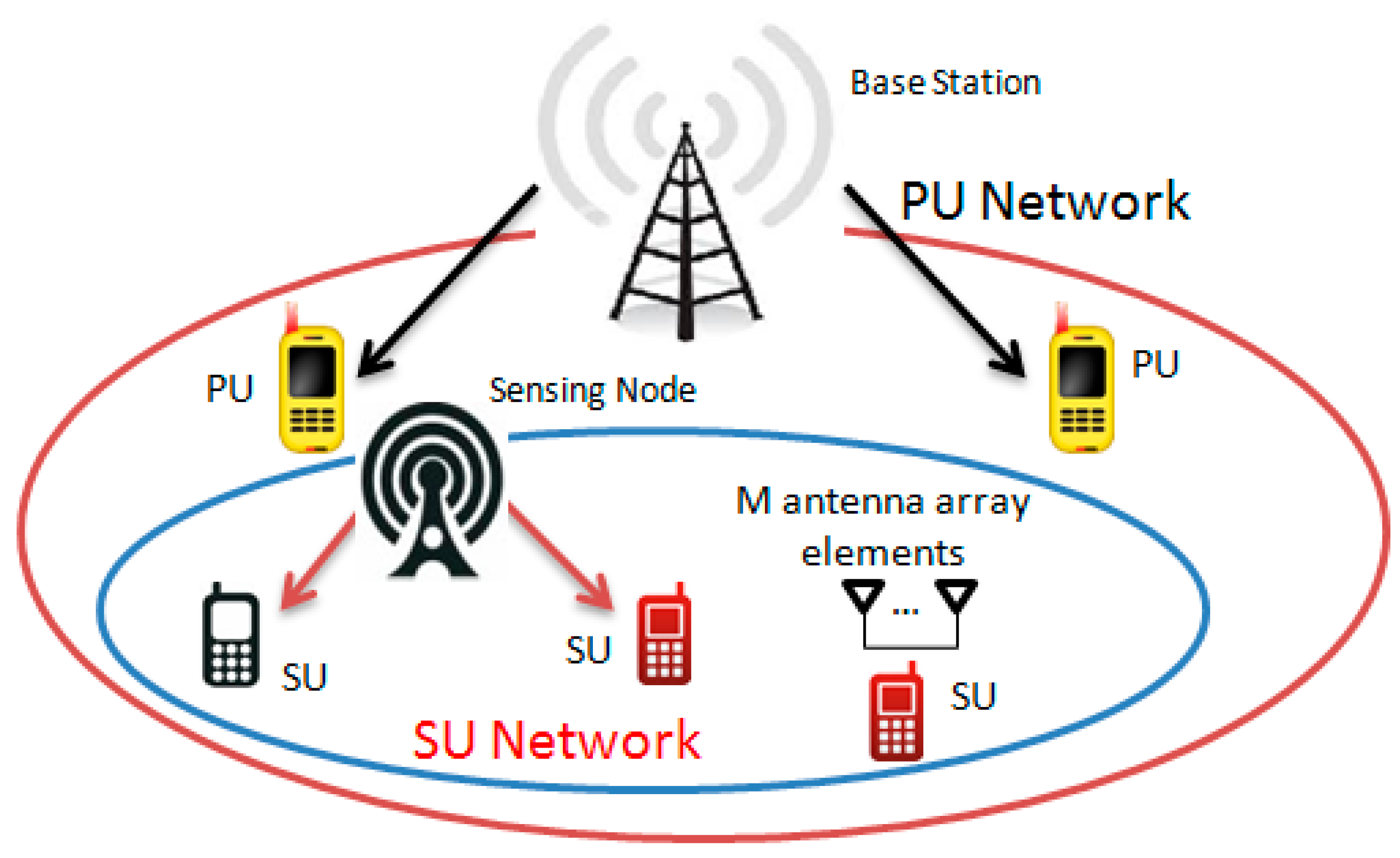
2.1. System Model
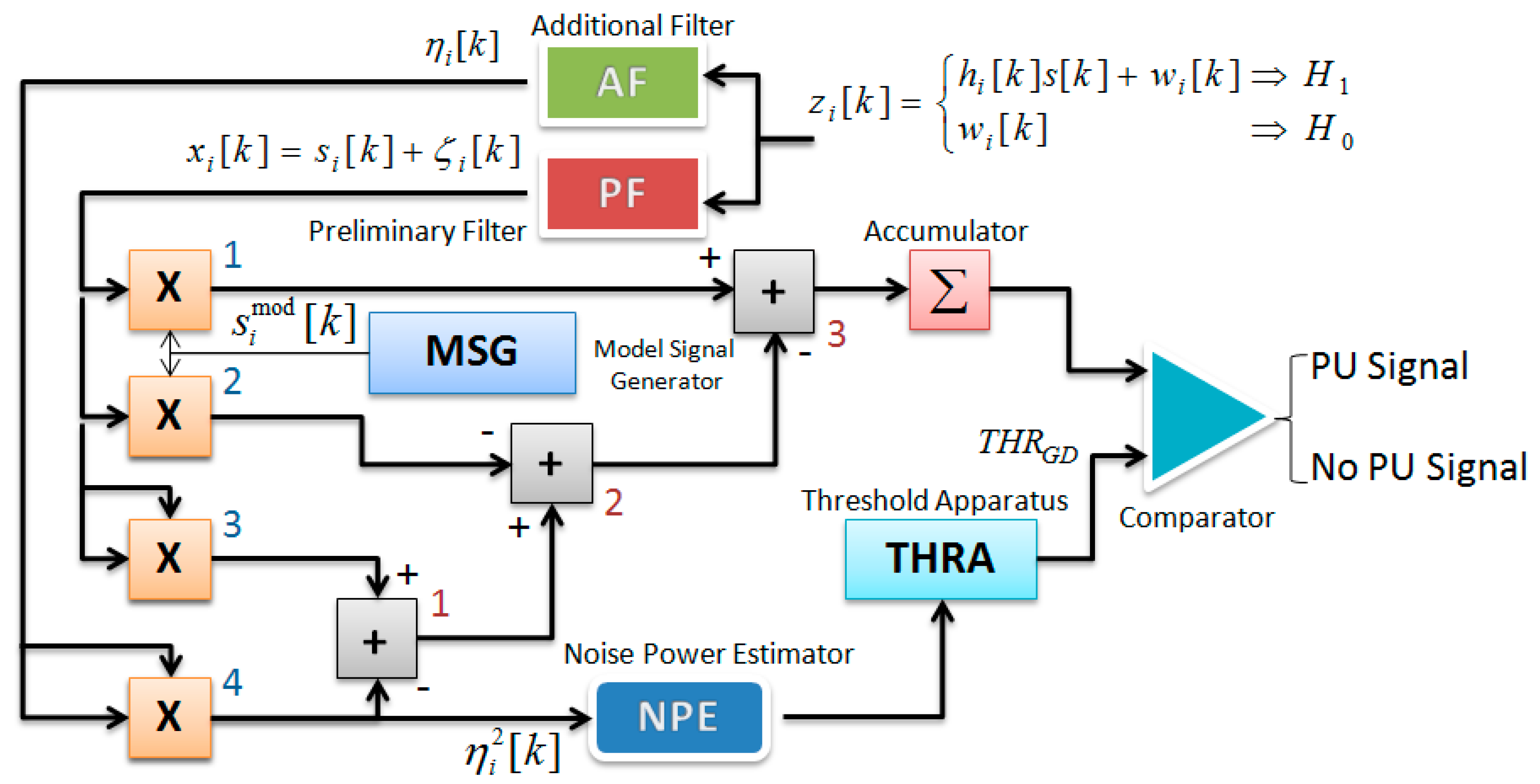
2.2. GD Statistics

- •
- The GD correlation channel—the PF, multipliers 1 and 2, model signal generator MSG;
- •
- The GD ED channel—the PF, AF, multipliers 3 and 4, summator 1;
- •
- The GD compensation channel—the summators 2 and 3 and accumulator Σ.

2.3. Moment Generation Function of the GD Partial Test Statistics
3. GD Spectrum Sensing and Sample Complexity
3.1. The Case

3.2. The Case
3.3. The GD Optimal Threshold
4. Simulation and Discussion

| Parameter | Value |
|---|---|
| Number of antenna array elements | |
| Signal-to-noise ratio | [dB] |
| Probability of false alarm | |
| Probability of miss | |
| Non-probabilistic uncertainty parameter | [dB] |
| Channel parameter | |
| Channel coherence time | |
| Fraction of the total power |


5. Conclusions
Acknowledgments
Author Contributions
Conflicts of Interest
Symbols and Variables Summary
| Symbol or Variable | Description | Symbol or Variable | Description |
| Non-probabilistic uncertainty parameter | Mean of the GD decision statistics under the hypothesis | ||
| Coefficient of spatial correlation | Variance of the GD decision statistics under the hypothesis | ||
| Fraction of the total power | Mean of the GD decision statistics under the hypothesis | ||
| Angular spread | Variance of the GD decision statistics under the hypothesis | ||
| Wavelength | GD detection threshold | ||
| Noise factor | GD optimal detection threshold | ||
| Amplitude factor | Probability of false alarm | ||
| Chi-square distribution degree of freedom | Probability of miss | ||
| Eigenvalue of the i-th spatial channel of the correlation matrix | GD probability of false alarm | ||
| Channel parameter | GD probability of miss | ||
| Noise variance | ED probability of false alarm | ||
| Noise variance at GD PF output | ED probability of miss | ||
| Noise variance at GD AF output | MF probability of false alarm | ||
| PU signal bandwidth | MF probability of miss | ||
| zero matrix | Probability of error | ||
| Antenna array element spacing | GD probability of error | ||
| Antenna array element correlation matrix | a priori probability of the PU signal absence | ||
| Covariance matrix under the hypothesis | a priori probability of the PU signal presence | ||
| Covariance matrix under the hypothesis | ED SNR wall | ||
| Average energy of transmitted signal | MF SNR wall | ||
| Hypothesis of signal absence | MF effective SNR | ||
| Hypothesis of signal presence | Discrete-time circularly symmetric complex Gaussian noise | ||
| Discrete-time channel coefficients | Stochastic process vector at the PF output | ||
| GD PF impulse response | Discrete-time signal at PF output | ||
| GD AF impulse response | Discrete-time received signal | ||
| Identity matrix | Noise at PF output | ||
| Channel coherence time | Noise at AF output | ||
| Number of antenna array elements | Signal vector | ||
| Number of samples (sample complexity) | Vector of the random process at the AF output | ||
| GD sample complexity | Vector of the process at the MSG output | ||
| ED sample complexity | Signal-to-noise ratio | ||
| MF sample complexity | GD decision statistics | ||
| PU Signal | Model signal |
Appendix A
Appendix B
References
- Sahai, A.; Hoven, N.; Tandra, R. Some fundamental limits on cognitive radio. In Proceedings of the 42nd Allerton Conference on Communication, Control, and Computing, Monticello, IL, USA, 29 September–1 October 2004; pp. 1662–1671.
- Tandra, R.; Sahai, A. Fundamental limits on detection in low SNR under noise uncertainty. In Proceedings of the 2005 IEEE International Conference on Wireless Networks, Communications and Mobile Computing, Maui, HI, USA, 13–16 June 2005; pp. 464–469.
- Tandra, R.; Sahai, A. SNR walls for signal detection. IEEE J. Sel. Top. Signal Process. 2008, 2, 4–17. [Google Scholar] [CrossRef]
- Ji, G.; Zhu, H. On the noise power uncertainty of the low SNR energy detection in cognitive radio. J. Comput. Inf. Syst. 2010, 6, 2457–2463. [Google Scholar]
- IEEE Std. 802.22–06/0088r0. Numerical Spectrum Sensing Requirements. June 2006. Available online: http://www.ieee802org/22/Meeting_documents/2005_June/22-06-0088-00-0000_Numerical_Spectrum_Sensing_Requirements.doc (accessed on 3 July 2015).
- Mariani, A.; Giorgetti, A.; Chiani, M. Effects of noise power estimation on energy detection for co-gnitive radio application. IEEE Trans. Commun. 2011, 59, 3410–3420. [Google Scholar] [CrossRef]
- Sonnenschein, A.; Fishman, P.M. Radiometric detection of spread spectrum signals in noise of uncertain power. IEEE Trans. Aerosp. Electron. Syst. 1992, 28, 654–660. [Google Scholar] [CrossRef]
- Yu, G.; Long, C.; Xiang, M.; Xi, W. A novel energy detection scheme based on dynamic threshold in cognitive radio systems. J. Comput. Inf. Syst. 2012, 8, 2245–2252. [Google Scholar]
- Jouini, W. Energy detection limits under log-normal approximated noise uncertainty. IEEE Signal Process. Lett. 2011, 18, 423–4261. [Google Scholar] [CrossRef]
- Alik, M.S.O.; Kokkeler, A.B.J.; Klumpernik, E.A.M.; Smit, G.J.M. Lowering the SNR wall for energy detection using cross-correlation. IEEE Trans. Veh. Technol. 2011, 60, 3748–3757. [Google Scholar]
- Tian, T.; Iwai, H.; Sasaoka, H. Energy detection using pseudo BER based SNR estimation scheme in cognitive radio. Sci. Engendering Rev. Doshisha Univ. 2012, 53, 45–52. [Google Scholar]
- Guibene, W.; Turki, M.; Hayar, A. Distribution discontinuities detection using algebraic technique for spectrum sensing cognitive radio networks. In Proceedings of the 5th International Conference on Cognitive Radio Oriented Wireless Networks and Communications, Cannes, France, 9–11 June 2010; pp. 1–5.
- Guibene, W.; Turki, M.; Zayen, B.; Hayar, A. Spectrum sensing for cognitive radio exploiting spectrum sensing discontinuities detection. EURASIP J. Wirel. Commun. Network. 2012. [Google Scholar] [CrossRef]
- Semiari, O.; Maham, B.; Yuen, C. On the effect of I/Q imbalance on energy detection and a novel four-level hypothesis spectrum sensing. IEEE Trans. Veh. Technol. 2014, 63, 4136–4141. [Google Scholar] [CrossRef]
- Deng, R.; Chen, J.; Yuen, C.; Cheng, P.; Sun, Y. Energy-Efficient cooperative spectrum sensing by optimal scheduling in sensor-aided cognitive radio networks. IEEE Trans. Veh. Technol. 2012, 61, 716–725. [Google Scholar] [CrossRef]
- Liu, Y.; Xie, S.; Yu, R.; Zhang, Y.; Yuen, C. An efficient MAC protocol with selective grouping and cooperative sensing in cognitive radio networks. IEEE Trans. Veh. Technol. 2013, 62, 3928–3941. [Google Scholar] [CrossRef]
- Tuzlukov, V. A new approach to signal detection theory. Digital Signal Process. 1998, 8, 166–184. [Google Scholar] [CrossRef]
- Tuzlukov, V. Signal Detection Theory; Springer-Verlag: Boston, MA, USA, 2001; p. 744. [Google Scholar]
- Tuzlukov, V. Signal Processing Noise; CRC Press, Taylor & Francis Group: Boca Raton, New York, WA, USA, 2002; p. 688. [Google Scholar]
- Shbat, M.S.; Tuzlukov, V. Evaluation of detection performance under employment of the generalized detector in radar sensor systems. Radioengineering 2014, 23, 50–65. [Google Scholar]
- Tuzlukov, V. Generalized approach to signal processing in wireless communications: The main aspects and some examples. In Wireless Communications and Networks: Recent Advances; Eksim, A., Ed.; InTech: Rijeka, Croatia, 2012; pp. 305–338. [Google Scholar]
- Tuzlukov, V. Communication Systems: New Research; NOVA Science Publishers, Inc.: New York, NY, USA, 2013; p. 423. [Google Scholar]
- Shbat, M.S.; Tuzlukov, V. Definition of adaptive detection threshold under employment of the generalized detector in radar sensor systems. IET Signal Process. 2014, 8, 622–632. [Google Scholar] [CrossRef]
- Shbat, M.S.; Tuzlukov, V. Spectrum sensing under correlated antenna array using generalized detector in cognitive radio systems. Int. J. Antennas Propag. 2013, 8. [Google Scholar] [CrossRef]
- Kim, S.; Lee, J.; Wang, H.; Hong, D. Sensing performance of energy detector with correlated multiple antennas. IEEE Signal. Process. Lett. 2009, 16, 671–674. [Google Scholar]
- Jun, M.; Li, Y.; Zhang, R.A.; Wang, R. A new spectrum sensing algorithm based on antenna correlation for cognitive radio systems. Wirel. Personal Commun. 2012, 66, 419–428. [Google Scholar] [CrossRef]
- Molisch, A.F.; Greenstein, L.J.; Shafi, M. Propagation issues for cognitive radio. IEEE Proc. 2009, 97, 787–804. [Google Scholar]
- Sun, H.; Laurenson, D.; Wang, C.X. Computationally tractable model of energy detection performance over slow fading channels. IEEE Commun. Lett. 2010, 14, 924–926. [Google Scholar]
- Chen, X.; Yuen, C. Efficient resource allocation in rateless-coded MU-MIMO cognitive radio network with QoS provisioning and limited feedback. IEEE Trans. Veh. Technol. 2013, 62, 395–399. [Google Scholar] [CrossRef]
- Loyka, S.L. Channel capacity of MIMO architecture using the exponential correlation matrix. IEEE Commun. Lett. 2001, 5, 369–371. [Google Scholar] [CrossRef]
- Maximov, M. Joint correlation of fluctuative noise at outputs of frequency filters. Radio Eng. 1956, 9, 28–38. [Google Scholar]
- Chernyak, Y. Joint correlation of noise voltage at outputs of amplifiers with nonoverlapping responses. Radio Phys. Electron. 1960, 4, 551–561. [Google Scholar]
- Cordeiro, C.; Challapali, K.; Birru, D.; Shankar, S. IEEE 802.22: An introduction to the first wireless standard based on cognitive radios. J. Commun. 2006, 1, 38–47. [Google Scholar] [CrossRef]
- Makarfi, A.U.; Hamdi, K.A. Interference analysis of energy detection for spectrum sensing. IEEE Trans. Veh. Technol. 2013, 62, 2570–2578. [Google Scholar] [CrossRef]
- Zhang, W.; Mallik, R.K.; Letaief, K.B. Optimization of cooperative spectrum sensing with energy detection in cognitive radio networks. IEEE Trans. Wirel. Commun. 2009, 8, 5761–5766. [Google Scholar] [CrossRef]
- Atapattu, S.; Tellambura, C.; Jiang, H. Spectrum sensing via energy detector in low SNR. In Proceedings of the IEEE International Conference on Communications (ICC 2011), Kyoto, Japan, 5–9 June 2011; pp. 1–5.
- Mishra, S.; Sahai, A.; Brodersen, R. Cooperative sensing among cognitive radios. In Proceedings of the 2006 IEEE International Conference on Communications (ICC’06), Istanbul, Turkey, 11–15 June 2006; pp. 1658–1663.
- Mariani, A.; Giorgetti, A.; Chiani, M. SNR wall for energy detection with noise power estimation. In Proceedings of the 2011 IEEE International Conference on Communications (ICC’11), Kyoto, Japan, 5–9 June 2011; pp. 1–6.
- Digham, F.F.; Alouini, M.-S.; Simon, M.K. On the energy detection of unknown signals over fad-ing channels. In Proceedings of the 2003 IEEE International Conference on Communications (ICC’03), Anchorage, AK, USA, 11–15 May 2003.
- Ghasemi, A.; Sousa, E.S. Spectrum sensing in cognitive radio networks: The cooperation-processing trade off. Wirel. Commun. Mob. Comput. 2007, 7, 1049–1060. [Google Scholar] [CrossRef]
- Ghasemi, A.; Sousa, E.S. Opportunistic spectrum access in fading channels through collaborative sensing. J. Commun. 2007, 2, 71–82. [Google Scholar] [CrossRef]
- Gradshteyn, D.C.; Ryzhik, I. Table of Integrals, Series, and Products, 7th ed.; Academic Press: London, UK, 2007. [Google Scholar]
- Alouini, M.S.; Abdi, A.; Kveh, M. Sum of gamma variates and performance of wireless communications systems over nakagami-fading channels. IEEE Trans. Veh. Technol. 2001, 50, 1471–1480. [Google Scholar] [CrossRef]
- Liang, Y.C.; Zeng, Y.; Peh, E.; Hoang, A.T. Sensing-throughput tradeoff for cognitive radio networks. IEEE Trans. Wirel. Commun. 2008, 7, 1326–1337. [Google Scholar] [CrossRef]
- Kate, S.K.; Navare, S.D.; Bandewar, S.R.; et al. Engineering Mathematics-II; Technical Publications Pune: Pune, India, 2007; Available online: http://www.adslwi-fi.com/aa.php?isbn=ISBN:8184311451&name=Engineering_Mathematics_-_Ii (accessed on 3 July 2015).
- Papadopoulos, A. Metric Spaces, Convexity and Non-Positive Curvature; European Mathematical Society Publishing House: Zurich, Switzerland, 2005; Available online: http://www.ems-ph.org (accessed on 3 July 2015).
© 2015 by the authors; licensee MDPI, Basel, Switzerland. This article is an open access article distributed under the terms and conditions of the Creative Commons Attribution license (http://creativecommons.org/licenses/by/4.0/).
Share and Cite
Shbat, M.S.; Tuzlukov, V. SNR Wall Effect Alleviation by Generalized Detector Employed in Cognitive Radio Networks. Sensors 2015, 15, 16105-16135. https://doi.org/10.3390/s150716105
Shbat MS, Tuzlukov V. SNR Wall Effect Alleviation by Generalized Detector Employed in Cognitive Radio Networks. Sensors. 2015; 15(7):16105-16135. https://doi.org/10.3390/s150716105
Chicago/Turabian StyleShbat, Modar Safir, and Vyacheslav Tuzlukov. 2015. "SNR Wall Effect Alleviation by Generalized Detector Employed in Cognitive Radio Networks" Sensors 15, no. 7: 16105-16135. https://doi.org/10.3390/s150716105