A Rapid Convergent Low Complexity Interference Alignment Algorithm for Wireless Sensor Networks

Abstract

Interference alignment (IA) is a novel technique that can effectively eliminate the interference and approach the sum capacity of wireless sensor networks (WSNs) when the signal-to-noise ratio (SNR) is high, by casting the desired signal and interference into different signal subspaces. The traditional alternating minimization interference leakage (AMIL) algorithm for IA shows good performance in high SNR regimes, however, the complexity of the AMIL algorithm increases dramatically as the number of users and antennas increases, posing limits to its applications in the practical systems. In this paper, a novel IA algorithm, called directional quartic optimal (DQO) algorithm, is proposed to minimize the interference leakage with rapid convergence and low complexity. The properties of the AMIL algorithm are investigated, and it is discovered that the difference between the two consecutive iteration results of the AMIL algorithm will approximately point to the convergence solution when the precoding and decoding matrices obtained from the intermediate iterations are sufficiently close to their convergence values. Based on this important property, the proposed DQO algorithm employs the line search procedure so that it can converge to the destination directly. In addition, the optimal step size can be determined analytically by optimizing a quartic function. Numerical results show that the proposed DQO algorithm can suppress the interference leakage more rapidly than the traditional AMIL algorithm, and can achieve the same level of sum rate as that of AMIL algorithm with far less iterations and execution time.

1. Introduction

Wireless sensor networks (WSNs) have received considerable attention, and have been applied to a large number of scenarios in recent years [1]. With the growth in network scale, interference management has become one of the major challenges in WSNs where multiple users often share some common resources simultaneously and high data rates are often demanded. A large amount of research has focused on interference management techniques in order to increase the sum rate of the system [2,3,4,5]. One recent interesting interference management scheme that can approach the channel capacity is interference alignment (IA), which was firstly studied by Maddah-Ali et al. [6] as well as Jafar and Shamai [7] for the multiple-input and multiple-output (MIMO) X channel. Subsequently, Cadambe and Jafar [8] proved that the throughput of the system varies linearly with the number of users in high signal-to-noise ratio (SNR) regimes by employing IA. In addition, the degrees of freedom (DoFs), which serve as one key measure of the channel capacity, were studied by Lee et al. [9] in the case of the MIMO Y channel and by Cadambe and Jafar [10] in the case of relay networks. Thanks to its bright prospects IA has been extended to use in many scenarios such as OFDM systems [11], femtocell networks [12], and cognitive networks [13,14]. In particular, Wu et al. [15] have leveraged the IA technique to mitigate the strong interference in large scale WSNs. In heterogeneous networks, Sharma et al. [16] have proposed a novel spectral coexistence mechanism which takes advantage of the IA technique.

Essentially, achieving IA is to design proper transmitting precoding matrices V to align the desired signal and interference to different signal subspaces, and to design proper receiving decoding matrices U to eliminate the interference at each receiver [17]. Tresch et al. [18] have developed closed-form solutions to IA for the MIMO interference channel with M + 1 users, one degree of freedom, M transmitting antennas, and M receiving antennas. However, the closed-form solutions to IA remain unknown except for some special situations [19]. Peters and Heath [20] have shown that it is difficult to formulate the closed-form solutions of V and U in the situation of more than three users. In addition, Razaviyayn et al. [21] have also shown that searching the optimal V and U is a nonconvex problem. Ma et al. [22] have performed a deep analysis on the computational complexity of interference alignment, and shown that the problem becomes NP-hard when the number of antennas at each node is larger than two. Therefore, many researchers [20,21,22,23,24,25,26] have focused on numerical methods to find the suboptimal V and U. Gomadam et al. [23] have leveraged the channel reciprocity and proposed the alternating minimization interference leakage (AMIL) and Max-SINR algorithms, which only require local channel state information (CSI). It has been shown by Xu et al. [27] that the AMIL and Max-SINR algorithms show close multiplexing gains in high SNR regimes and the former approach has lower complexity than the latter one. A similar alternating minimization IA algorithm has been proposed in [20] without assuming the network reciprocity. Shen et al. [24] have developed the minimum mean square error (MMSE) IA algorithm for the case of imperfect CSI. A sequential antenna switch algorithm was proposed in [28], in which the quality of service of the IA system was considered.

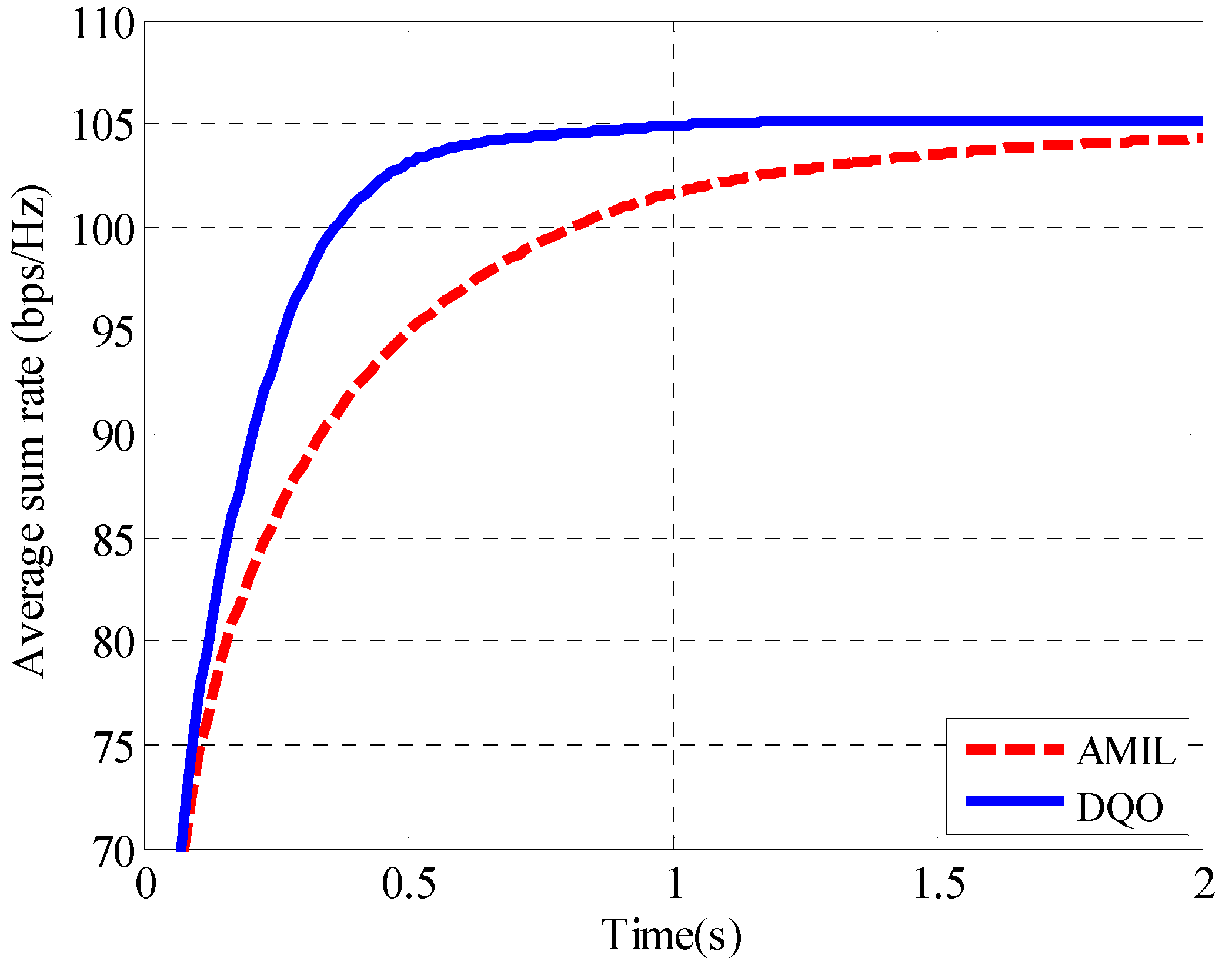
Among these methods, the AMIL algorithm can suppress the interference leakage to a low level and thus can achieve high throughput in high SNR regimes where the sum rate of the system is determined by interference instead of noise. However, it might take a large number of iterations as well as long computational time in the case of large numbers of users and antennas. Furthermore, for the reason that CSI is time-variable, the practical IA system has limited computational time, which will certainly become the bottleneck of the implementation of AMIL algorithm when there are plenty of users and antennas. In this paper, we investigate the properties of the AMIL algorithm, and discover that the difference between the consecutive iteration results of the AMIL algorithm will approximately point to the convergence solution when the precoding and decoding matrices obtained from the intermediate iterations are sufficiently close to their convergence values. Based on this property, we propose a rapidly convergent low-complexity IA algorithm, i.e., directional quartic optimal (DQO) algorithm. It leverages a line search (LS) optimization method, which iteratively generates searching directions and optimal step sizes. The searching direction is obtained by subtracting the consecutive results of AMIL algorithm, and the optimal step size is calculated by solving a quartic optimization problem.

The rest of the paper is organized as follows: in Section 2, we describe the system model. The properties of the AMIL algorithm are studied in Section 3, which will serve as the foundation of the algorithm proposed later. In Section 4, the DQO algorithm is proposed, and the corresponding procedure, optimal step size calculation, and complexity analysis are provided. Numerical results to evaluate the proposed algorithm are presented and discussed in Section 5. Finally, the paper is concluded in Section 6. As far as the notation used in the paper is concerned, we employ (M × N, d)^K to represent a K-user MIMO interference channel where each user wishes to transmit d data streams with M transmitting antennas and N receiving antennas. We use C, R, C^M×N, I, and CN(μ, σ²) to represent the complex domain, the real domain, the M × N complex matrix, the identity matrix, and the complex Gaussian distribution with mean μ and variance σ², respectively. Re{a} denotes the real part of scalar a. A^T, A*, A^H, ||A||, Tr[A] and A_*(l) mean the transpose, the conjugate, the conjugate transpose, the Frobenius norm, the trace and the l-th column of matrix A, respectively. eig_l[A] stands for the eigenvector associated with the l-th smallest eigenvalue of matrix A. We employ Aⁱ to represent the value of A at the i-th iterations. diag(a₁, a₂, ..., a_m) represents a diagonal matrix with its diagonal elements equal to a₁, a₂, …, a_m.

2. System Model

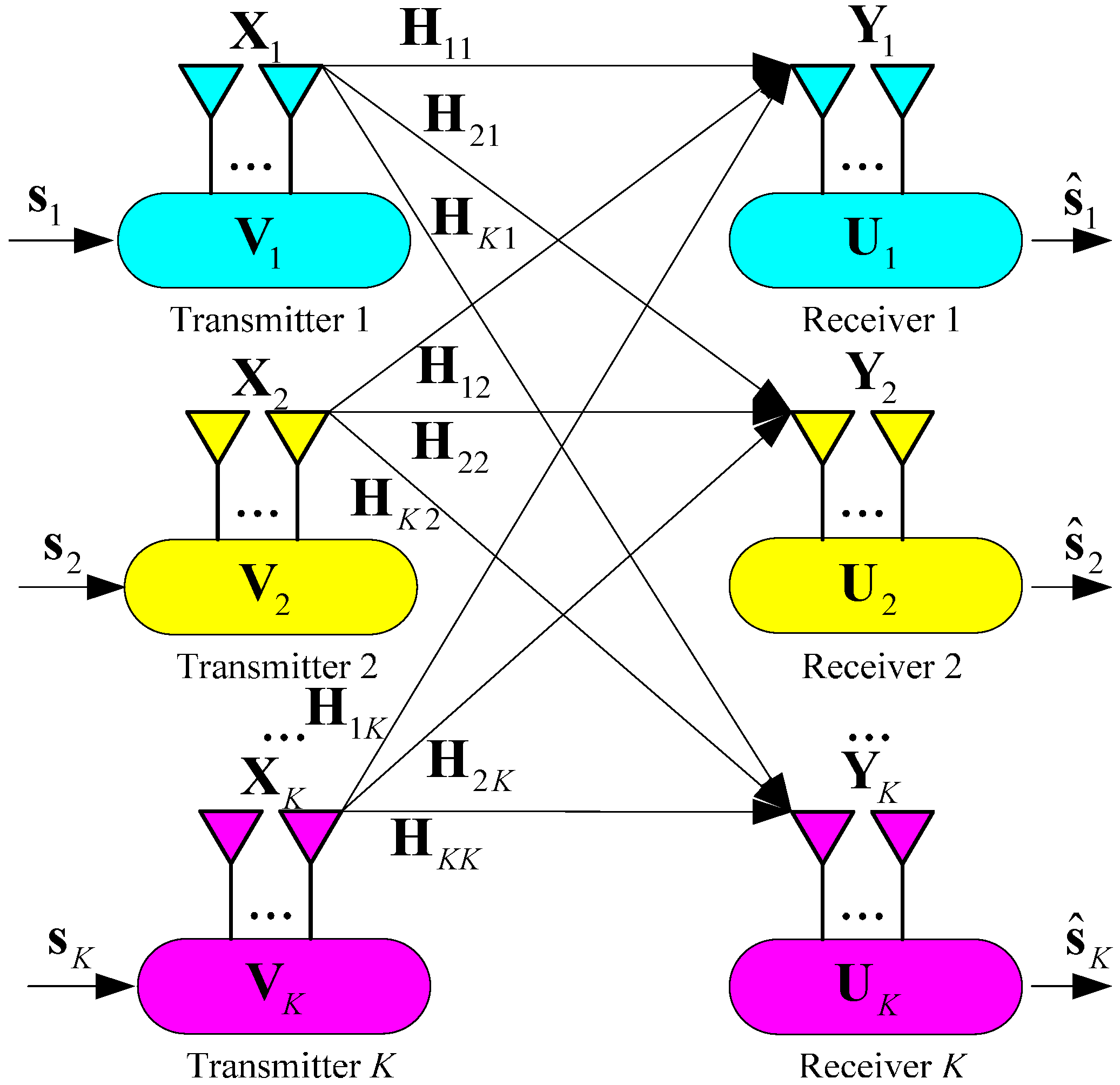
In this paper, the (M × N, d)^K MIMO interference channel is considered, and is depicted in Figure 1. The received signal of the k-th user can be represented as [23]:

$$Y_k={\displaystyle \sum _{l=1}^K{H}_{kl}{V}_l{s}_l}+n_k,k\in 1,2,\mathrm{...},K$$

(1)

where s_k ∈ C^d×1, V_k ∈ C^M×d, and Y_k ∈ C^N×1 denote the data vector, the precoding matrix, and the received signal vector of the k-th user, respectively; n_k ∈ C^N×1 represents the noise vector with distribution of CN(0, σ²) for each element; H_kl ∈ C^N×M represents the channel matrix from transmitter l to receiver k. In the network we considered, CSI is obtained through CSI feedback, which serves as one critical technique in IA. A large number of researchers such as Ayach [29], Cho [30], and Zhang [31] have focused on the CSI feedback strategy. Since we mainly focus on designing the precoding and decoding matrices, further investigation on CSI feedback is beyond the scope of the paper and an accurate global CSI is assumed to be available at each node throughout this paper.

Figure 1. System model of the K-user MIMO interference channel.

Figure 1. System model of the K-user MIMO interference channel.

The k-th user’s covariance matrices of the forward and reciprocal networks are respectively given by:

$$Q_k={\displaystyle \sum _{l=1,l\ne k}^K\frac{P_l}{d}}{H}_{kl}{V}_l{V}_l^{\text{H}}{H}_{kl}^{\text{H}}$$

(2)

$${\overleftarrow{Q}}_k={\displaystyle \sum _{l=1,l\ne k}^K\frac{{\overleftarrow{P}}_l}{d}}{H}_{lk}^{\text{H}}{U}_l{U}_l^{\text{H}}{H}_{lk}$$

(3)

where P_l and $\overleftarrow{P}$ denote the transmitting power of the l-th user in the forward and the reciprocal networks, respectively. Then the interference leakage at receiver k can be calculated as:

$$L_k=\text{Tr}[U_k^{\text{H}}{Q}_k{U}_k]$$

(4)

where U_k ∈ C^N×d is the decoding matrix at receiver k. The total interference leakage is defined as the sum of the leakage at each receiver, i.e.,:

$$L={\displaystyle \sum _{k=1}^K{L}_k}$$

(5)

Then the minimal interference leakage problem is to design proper transmitting precoding matrices V and receiving decoding matrices U to minimize Equation (5) under the following constraints:

$$\text{rank}(U_k^{\text{H}}{H}_{kk}{V}_k)=d$$

(6)

$$V_k^{\text{H}}{V}_k=I,U_k^{\text{H}}{U}_k=I$$

(7)

The former constraint guarantees the feasibility of the desired signal reconstruction and the later one ensures the uniqueness of the IA solution [17].

3. Properties of AMIL Algorithm

The AMIL algorithm, whose procedure is summarized in Algorithm 1, was proposed by Gomadam et al. [23] to find the IA solution by exploiting the channel reciprocity. In this section, we investigate the properties of the AMIL algorithm, and show that the difference of the consecutive iteration results of AMIL algorithm will approximately point to the convergence solution when the precoding and decoding matrices obtained from the intermediate iterations are sufficiently close to their convergence values. This interesting property will serve as the foundation of the algorithm proposed later.

Algorithm 1 AMIL Algorithm

Initialize Lth, Imax, and $V_k^0$, with ${(V_k^0)}^{\text{H}}{V}_k^0=I$ (k = 1, 2,…, K). i = 0. Repeat i = i + 1 (VU-step):Calculate $Q_k^i$ according to Equation (2). Update $U_k^i$ so that $U_{k(l)}^i={\text{eig}}_l[Q_k^i],l=1,2,\mathrm{..},d.$ (UV-step):Calculate $\overleftarrow{Q_k^i}$ according to Equation (3). Update $V_k^i$ so that $V_{k(l)}^i={\text{eig}}_l[\overleftarrow{Q_k^i}],l=1,2,\mathrm{..},d.$ Calculate the interference leakage L according to Equation (5). Until L < Lth or i > Imax.

As shown in Algorithm 1, the AMIL algorithm calculates the optimal decoding matrices U by fixing V in the forward channel, and computes the optimal V by fixing U in the reciprocal channel. It can monotonously suppress the interference leakage, and has been proved to converge to a local minimum. Although the convergence point is not guaranteed to be the optimal IA solution, it has been verified numerically that in many cases AMIL algorithm can achieve a low interference leakage level after sufficient iterations. Therefore, in high SNR regimes, where the sum rate is limited by interference rather than noise, the AMIL algorithm serves as a good method to increase the sum rate. In addition, the procedure of alternating minimization is very effective, and is often employed by many other algorithms. In spite of this, the iterations as well as time required by AMIL algorithm to reach a certain level of interference leakage increase dramatically with the number of users and antennas. Therefore, the properties of AMIL algorithm are studied in order to figure out a way to increase the convergence rate and thus to reduce its complexity as well as the required computational time.

Throughout this paper, $V_k^i$ ∈ C^M×d and $U_k^i$ ∈ C^N×d are employed to represent the k-th user’s precoding and decoding matrices obtained from the i-th iteration, respectively. The convergence value of $V_k^i$ and $U_k^i$ are defined as ${\tilde{V}}_k$ and ${\tilde{U}}_k$, respectively. Define $\mathrm{\Delta }{V}_k^i$ ∈ C^M×d as the deviation from $V_k^i$ to ${\tilde{V}}_k$, and $\mathrm{\Delta }{U}_k^i$ ∈ C^N×d as the deviation from $U_k^i$ to ${\tilde{U}}_k$ so that:

$$V_k^i={\tilde{V}}_k+\mathrm{\Delta }{V}_k^i$$

(8)

$$U_k^i={\tilde{U}}_k+\mathrm{\Delta }{U}_k^i$$

(9)

Define ${\overline{V}}^i$, $\overline{\tilde{V}}$, $\mathrm{\Delta }{\overline{V}}^i$∈ C^MdK×1 and ${\overline{U}}^i$, $\overline{\tilde{U}}$, $\mathrm{\Delta }{\overline{U}}^i$∈ C^NdK×1 as:

$${\overline{V}}^i=\left[\begin{array}{l}{V}_{1(1)}^i\hfill \\ V_{1(2)}^i\hfill \\ \mathrm{...}\hfill \\ V_{1(d)}^i\hfill \\ \mathrm{...}\hfill \\ V_{K(1)}^i\hfill \\ V_{K(2)}^i\hfill \\ \mathrm{...}\hfill \\ V_{K(d)}^i\hfill \end{array}\right],\overline{\tilde{V}}=\left[\begin{array}{l}{\tilde{V}}_{1(1)}\hfill \\ {\tilde{V}}_{1(2)}\hfill \\ \mathrm{...}\hfill \\ {\tilde{V}}_{1(d)}\hfill \\ \mathrm{...}\hfill \\ {\tilde{V}}_{K(1)}\hfill \\ {\tilde{V}}_{K(2)}\hfill \\ \mathrm{...}\hfill \\ {\tilde{V}}_{K(d)}\hfill \end{array}\right],\mathrm{\Delta }{\overline{V}}^i=\left[\begin{array}{l}\mathrm{\Delta }{V}_{1(1)}^i\hfill \\ \mathrm{\Delta }{V}_{1(2)}^i\hfill \\ \mathrm{...}\hfill \\ \mathrm{\Delta }{V}_{1(d)}^i\hfill \\ \mathrm{...}\hfill \\ \mathrm{\Delta }{V}_{K(1)}^i\hfill \\ \mathrm{\Delta }{V}_{K(2)}^i\hfill \\ \mathrm{...}\hfill \\ \mathrm{\Delta }{V}_{K(d)}^i\hfill \end{array}\right],{\overline{U}}^i=\left[\begin{array}{l}{U}_{1(1)}^i\hfill \\ U_{1(2)}^i\hfill \\ \mathrm{...}\hfill \\ U_{1(d)}^i\hfill \\ \mathrm{...}\hfill \\ U_{K(1)}^i\hfill \\ U_{K(2)}^i\hfill \\ \mathrm{...}\hfill \\ U_{K(d)}^i\hfill \end{array}\right],\overline{\tilde{U}}=\left[\begin{array}{l}{\tilde{U}}_{1(1)}\hfill \\ {\tilde{U}}_{1(2)}\hfill \\ \mathrm{...}\hfill \\ {\tilde{U}}_{1(d)}\hfill \\ \mathrm{...}\hfill \\ {\tilde{U}}_{K(1)}\hfill \\ {\tilde{U}}_{K(2)}\hfill \\ \mathrm{...}\hfill \\ {\tilde{U}}_{K(d)}\hfill \end{array}\right],\mathrm{\Delta }{\overline{U}}^i=\left[\begin{array}{l}\mathrm{\Delta }{U}_{1(1)}^i\hfill \\ \mathrm{\Delta }{U}_{1(2)}^i\hfill \\ \mathrm{...}\hfill \\ \mathrm{\Delta }{U}_{1(d)}^i\hfill \\ \mathrm{...}\hfill \\ \mathrm{\Delta }{U}_{K(1)}^i\hfill \\ \mathrm{\Delta }{U}_{K(2)}^i\hfill \\ \mathrm{...}\hfill \\ \mathrm{\Delta }{U}_{K(d)}^i\hfill \end{array}\right]$$

(10)

From Equations (8) and (9), it can be obtained that:

$${\overline{V}}^i=\overline{\tilde{V}}+\mathrm{\Delta }{\overline{V}}^i$$

(11)

$${\overline{U}}^i=\overline{\tilde{U}}+\mathrm{\Delta }{\overline{U}}^i$$

(12)

The investigation begins with the linear transformation property of AMIL algorithm as follows:

Theorem 1.

If AMIL algorithm can converge to a point where the interference leakage is very small, there exist fixed linear transformations T_V and T_U, which do not change with iterations. When ${\overline{V}}^i$ and ${\overline{U}}^i$ are sufficiently close to $\overline{\tilde{V}}$ and $\overline{\tilde{U}}$, respectively, the deviations of the (i + 1)-th iteration can be approximated as follows:

$$\mathrm{\Delta }{\overline{V}}^{i+1}\approx T_{\text{V}}\mathrm{\Delta }{\overline{V}}^i$$

(13)

$$\mathrm{\Delta }{\overline{U}}^{i+1}\approx T_{\text{U}}\mathrm{\Delta }{\overline{U}}^i$$

(14)

Proof of Theorem 1.

In the situation when AMIL algorithm converges to a point where the interference leakage is very small, which is easy to achieve for AMIL algorithm, we have:

$${\tilde{U}}_j^{\text{H}}{H}_{ji}{\tilde{V}}_i\approx 0,j\ne i$$

(15)

Define the interference covariance matrices at the convergence point as:

$${\tilde{Q}}_k={\displaystyle \sum _{j=1,j\ne k}^K{H}_{kj}{\tilde{V}}_j}{\tilde{V}}_j^{\text{H}}{H}_{kj}^{\text{H}}$$

(16)

$${\overleftarrow{\tilde{Q}}}_k={\displaystyle \sum _{j=1,j\ne k}^K{H}_{jk}^{\text{H}}{\tilde{U}}_j}{\tilde{U}}_j^{\text{H}}{H}_{jk}$$

(17)

Assume that the l-th smallest eigenvalue and the associated eigenvector of ${\tilde{Q}}_k$ are $\overleftarrow{{\lambda }_{k,l}}$ and ${\overleftarrow{\nu }}_{k,l}$, respectively. Similarly for ${\overleftarrow{\tilde{Q}}}_k$, we have ${\lambda }_{k,l}$ and ${\nu }_{k,l}$. From the procedure of AMIL algorithm, ${\tilde{V}}_k$ and ${\tilde{U}}_k$ should be the eigenvectors corresponding to the d smallest eigenvalues of ${\overleftarrow{\tilde{Q}}}_k$ and ${\tilde{Q}}_k$, respectively. Therefore, ${\tilde{V}}_k$ and ${\tilde{U}}_k$ can be respectively given by:

$${\tilde{V}}_k=[{\nu }_{k,1},{\nu }_{k,2},\mathrm{...},{\nu }_{k,d}]$$

(18)

$${\tilde{U}}_k=[{\overleftarrow{\nu }}_{k,1},{\overleftarrow{\nu }}_{k,2},\mathrm{...},{\overleftarrow{\nu }}_{k,d}]$$

(19)

At the (i + 1)-th iteration, the VU-step of AMIL algorithm is performed on the precoding matrices $\left\{V_k^i\right\}$ and covariance matrix at the (i + 1)-th iteration can be expressed as:

$$\begin{array}{cc}{Q}_k^{i+1}& ={\displaystyle \sum _{j=1,j\ne k}^K{H}_{kj}{V}_j^i{V}_j^{i\text{H}}{H}_{kj}^{\text{H}}}\\ & ={\displaystyle \sum _{j=1,j\ne k}^K{H}_{kj}[{\tilde{V}}_j+\mathrm{\Delta }{V}_j^i}]{[{\tilde{V}}_j+\mathrm{\Delta }{V}_j^i]}^{\text{H}}{H}_{kj}^{\text{H}}\\ & \text{=}{\tilde{Q}}_k\text{+}\mathrm{\Delta }{Q}_k^{i+1}\end{array}$$

(20)

where $\mathrm{\Delta }{Q}_k^{i+1}$ is given by:

$$\mathrm{\Delta }{Q}_k^{i+1}={\displaystyle \sum _{j=1,j\ne k}^K{H}_{kj}[\mathrm{\Delta }{V}_j^i}{\tilde{V}}_j^{\text{H}}+{\tilde{V}}_j\mathrm{\Delta }{V}_j^{i\text{H}}+\mathrm{\Delta }{V}_j^i\mathrm{\Delta }{V}_j^{i\text{H}}]H_{kj}^{\text{H}}$$

(21)

When ${\overline{V}}^i$ and ${\overline{U}}^i$ are sufficiently close to $\overline{\tilde{V}}$ and $\overline{\tilde{U}}$ respectively, the deviation $\mathrm{\Delta }{V}_j^i$ is very small. Therefore, the high order term $\mathrm{\Delta }{V}_j^i\mathrm{\Delta }{V}_j^{i\text{H}}$ can be ignored, and Equation (21) can be simplified as:

$$\mathrm{\Delta }{Q}_k^{i+1}\approx {\displaystyle \sum _{j=1,j\ne k}^K{H}_{kj}[\mathrm{\Delta }{V}_j^i}{\tilde{V}}_j^{\text{H}}+{\tilde{V}}_j\mathrm{\Delta }{V}_j^{i\text{H}}]H_{kj}^{\text{H}}$$

(22)

According to the AMIL algorithm, ${\text{U}}_k^{i+1}$ should be the eigenvector corresponding to the d smallest eigenvalues of $Q_k^{i+1}$. From Equations (19) and (20), using the Eigenvalue Perturbation Theory, the l-th column of $U_k^{i+1}$ can be approximated by:

$$\begin{array}{cc}{U}_{k(l)}^{i+1}& \approx {\overleftarrow{\nu }}_{k,l}+{\displaystyle \sum _{j=1,j\ne l}^N\frac{{\overleftarrow{\nu }}_{k,j}^{\text{H}}\mathrm{\Delta }{Q}_k^{i+1}{\overleftarrow{\nu }}_{k,l}}{\overleftarrow{{\lambda }_{k,l}}-\overleftarrow{{\lambda }_{k,j}}}{\overleftarrow{\nu }}_{k,j}}\\ & ={\tilde{U}}_{k(l)}+{\displaystyle \sum _{j=1,j\ne l}^N\frac{{\overleftarrow{\nu }}_{k,j}^{\text{H}}\mathrm{\Delta }{Q}_k^{i+1}{\tilde{U}}_{k(l)}}{\overleftarrow{{\lambda }_{k,l}}-\overleftarrow{{\lambda }_{k,j}}}{\overleftarrow{\nu }}_{k,j}}\\ & ={\tilde{U}}_{k(l)}+\mathrm{\Delta }{U}_{k(l)}^{i+1}\end{array}$$

(23)

where $\mathrm{\Delta }{U}_{k(l)}^{i+1}$ is given by:

$$\mathrm{\Delta }{U}_{k(l)}^{i+1}={\displaystyle \sum _{j=1,j\ne l}^N\frac{{\overleftarrow{\nu }}_{k,j}^{\text{H}}\mathrm{\Delta }{Q}_k^{i+1}{\tilde{U}}_{k(l)}}{\overleftarrow{{\lambda }_{k,l}}-\overleftarrow{{\lambda }_{k,j}}}{\overleftarrow{\nu }}_{k,j}}$$

(24)

Substitute Equation (22) into (24), and $\mathrm{\Delta }{U}_{k(l)}^{i+1}$ can be rewritten as:

$$\mathrm{\Delta }{U}_{k(l)}^{i+1}\approx {\displaystyle \sum _{j=1,j\ne l}^N\frac{1}{\overleftarrow{{\lambda }_{k,l}}-\overleftarrow{{\lambda }_{k,j}}}}{\overleftarrow{\nu }}_{k,j}^{\text{H}}\{{\displaystyle \sum _{r=1,r\ne k}^K{H}_{kr}}[\mathrm{\Delta }{V}_r^i{\tilde{V}}_r^{\text{H}}+{\tilde{V}}_r\mathrm{\Delta }{V}_r^{i\text{H}}]H_{kr}^{\text{H}}\}{\tilde{U}}_{k(l)}{\overleftarrow{\nu }}_{k,j}$$

(25)

From Equation (15), the terms ${\tilde{V}}_r^{\text{H}}{H}_{kr}^{\text{H}}{\tilde{U}}_{k(l)}$ in Equation (25) is approximately zero and thus can be omitted. Therefore, Equation (25) can be simplified as:

$$\mathrm{\Delta }{U}_{k(l)}^{i+1}\approx {\displaystyle \sum _{j=1,j\ne l}^N\frac{{\overleftarrow{\nu }}_{k,j}^{\text{H}}{\displaystyle \sum _{r=1,r\ne k}^K{H}_{kr}{\tilde{V}}_r\mathrm{\Delta }{V}_r^{i\text{H}}}{H}_{kr}^{\text{H}}{\tilde{U}}_{k(l)}}{\overleftarrow{{\lambda }_{k,l}}-\overleftarrow{{\lambda }_{k,j}}}{\overleftarrow{\nu }}_{k,j}}$$

(26)

From Equation (26), it can be seen that $\mathrm{\Delta }{U}_{k(l)}^{i+1}$ is approximately the linear combination of the elements of ${(\mathrm{\Delta }{V}_r^i)}^{\ast }$, and the coefficients of the combination are corresponding to ${\overleftarrow{\nu }}_{k,j}^{\text{H}}$, $H_{kr}$, ${\tilde{V}}_r$, ${\tilde{U}}_k$ and $\overleftarrow{{\lambda }_{k,j}}$, which are fixed and do not vary with iterations i. Hence there exists a fixed matrix T_VU ∈ C^{NKd × MKd} which does not change with iterations, so that:

$$\mathrm{\Delta }{\overline{U}}^{i+1}\approx T_{\text{VU}}\cdot {(\mathrm{\Delta }{\overline{V}}^i)}^{\ast }$$

(27)

Similarly for the UV-step, there exists a fixed matrix T_UV ∈ C^{MKd × NKd} which does not change with iterations, so that:

$$\mathrm{\Delta }{\overline{V}}^{i+1}\approx T_{\text{UV}}\cdot {(\mathrm{\Delta }{\overline{U}}^{i+1})}^{\ast }$$

(28)

From Equations (27) and (28), we have:

$$\mathrm{\Delta }{\overline{V}}^{i+1}\approx T_{\text{UV}}{T}_{\text{VU}}^{\ast }\cdot \mathrm{\Delta }{\overline{V}}^i=T_{\text{V}}\mathrm{\Delta }{\overline{V}}^i$$

(29)

$$\mathrm{\Delta }{\overline{U}}^{i+1}\approx T_{\text{VU}}{T}_{\text{UV}}^{\ast }\cdot \mathrm{\Delta }{\overline{U}}^i=T_{\text{U}}\mathrm{\Delta }{\overline{U}}^i$$

(30)

where:

$$T_{\text{V}}=T_{\text{UV}}{T}_{\text{VU}}^{\ast }\in {ℂ}^{MKd\times MKd}$$

(31)

$$T_{\text{U}}=T_{\text{VU}}{T}_{\text{UV}}^{\ast }\in {ℂ}^{NKd\times NKd}$$

(32)

It can be seen that T_V and T_U determine the properties of AMIL algorithm when the current point is sufficiently close to its convergence value. As the analytical forms of T_V and T_U are extremely complex, the features of these two transformations are investigated by simulation and one interesting property observed is given as follows:

Property 1.

In the case of (M × M, d)^K channel, there exist two nonsingular matrices P_V and P_U, so that T_V and T_U can be expressed as:

$$T_{\text{V}}=P_{\text{V}}^{-1}\mathrm{\Lambda }{P}_{\text{V}}$$

(33)

$$T_{\text{U}}=P_{\text{U}}^{-1}\mathrm{\Lambda }{P}_{\text{U}}$$

(34)

where Λ = diag(κ₁, κ₂,…, κ_MKd) with κ₁ > κ₂ ... > κ_r and κ_{r + 1} = κ_{r + 2} = ... = κ_MKd = 0 (1 < r < KMd).

Based on the properties above, we further study the situation when consecutive applications of T_V and T_U are exerted on the deviation, and come to the following theorem.

Theorem 2.

In the (M × M, d)^K channel, if AMIL algorithm can converge to a point where the interference leakage is very small, the convergence solutions ${\tilde{V}}_k$ and ${\tilde{U}}_k$ (k = 1, 2, ..., K) can be approximated by the following Equations (35) and (36), when $V_k^i$ and $U_k^i$ are sufficiently close to ${\tilde{V}}_k$ and ${\tilde{U}}_k$, respectively :

$${\tilde{V}}_k\approx V_k^i+t(V_k^i-V_k^{i-1}),t\in ℝ$$

(35)

$${\tilde{U}}_k\approx U_k^i+t(U_k^i-U_k^{i-1})$$

(36)

Proof of Theorem 2.

At the (i + i₁)-th iteration, from Equations (29), (30), (33) and (34), we have:

$$\begin{array}{cc}\mathrm{\Delta }{\overline{V}}^{i+i_1}& \approx T_{\text{V}}^{i_1}\mathrm{\Delta }{\overline{V}}^i\\ & =P_{\text{V}}^{-1}{\mathrm{\Lambda }}^{i_1}{P}_{\text{V}}\mathrm{\Delta }{\overline{V}}^i\\ & =P_{\text{V}}^{-1}diag({\kappa }_1^{i_1},{\kappa }_2^{i_1},\mathrm{...},{\kappa }_{MKd}^{i_1})P_{\text{V}}\mathrm{\Delta }{\overline{V}}^i\end{array}$$

(37)

$$\begin{array}{cc}\mathrm{\Delta }{\overline{U}}^{i+i_1}& \approx T_{\text{U}}^{i_1}\mathrm{\Delta }{\overline{U}}^i\\ & =P_{\text{U}}^{-1}{\mathrm{\Lambda }}^{i_1}{P}_{\text{U}}\mathrm{\Delta }{\overline{U}}^i\\ & =P_{\text{U}}^{-1}diag({\kappa }_1^{i_1},{\kappa }_2^{i_1},\mathrm{...},{\kappa }_{MKd}^{i_1})P_{\text{U}}\mathrm{\Delta }{\overline{U}}^i\end{array}$$

(38)

Define e_k, g_k ∈ C^MKd×1 and f_k, s_k ∈ C so that:

$$P_{\text{V}}^{-1}=[e_1,e_2,\mathrm{...},e_{MKd}]$$

(39)

$$P_{\text{U}}^{-1}=[g_1,g_2,\mathrm{...},g_{MKd}]$$

(40)

$$P_{\text{V}}\mathrm{\Delta }{\overline{V}}^i={[f_1,f_2,\mathrm{...},f_{MKd}]}^{\text{T}}$$

(41)

$$P_{\text{U}}\mathrm{\Delta }{\overline{U}}^i={[h_1,h_2,\mathrm{...},h_{MKd}]}^{\text{T}}$$

(42)

Thus Equations (37) and (38) can be written as:

$$\mathrm{\Delta }{\overline{V}}^{i+i_1}\approx {\displaystyle \sum _{j=1}^{MKd}{\kappa }_j^{i_1}{f}_j{e}_j}$$

(43)

$$\mathrm{\Delta }{\overline{U}}^{i+i_1}\approx {\displaystyle \sum _{j=1}^{MKd}{\kappa }_j^{i_1}{h}_j{g}_j}$$

(44)

According to Property 1, when i₁ is large enough, it can be obtained that:

$${\kappa }_1^{i_1}\gg {\kappa }_2^{i_1}\gg \mathrm{...}\gg {\kappa }_r^{i_1},{\kappa }_{r+1}^{i_1}={\kappa }_{r+2}^{i_1}=\mathrm{...}={\kappa }_{MKd}^{i_1}=0$$

(45)

Therefore, Equations (43) and (44) can be approximated by:

$$\mathrm{\Delta }{\overline{V}}^{i+i_1}\approx {\kappa }_1^{i_1}{f}_1{e}_1$$

(46)

$$\mathrm{\Delta }{\overline{U}}^{i+i_1}\approx {\kappa }_1^{i_1}{h}_1{g}_1$$

(47)

At the (i + i₁ + 1)-th iteration, it can be obtained that:

$$\mathrm{\Delta }{\overline{V}}^{i+i_1+1}\approx {\kappa }_1^{i_1+1}{f}_1{e}_1\approx {\kappa }_1\mathrm{\Delta }{\overline{V}}^{i+i_1}$$

(48)

$$\mathrm{\Delta }{\overline{U}}^{i+i_1+1}\approx {\kappa }_1^{i_1+1}{h}_1{g}_1\approx {\kappa }_1\mathrm{\Delta }{\overline{U}}^{i+i_1}$$

(49)

From Equations (11), (12), (48) and (49), we have:

$$\overline{\tilde{V}}={\overline{V}}^{i+i_1+1}-\mathrm{\Delta }{\overline{V}}^{i+i_1+1}\approx {\overline{V}}^{i+i_1+1}+\frac{{\kappa }_1}{1-{\kappa }_1}(\mathrm{\Delta }{\overline{V}}^{i+i_1+1}-\mathrm{\Delta }{\overline{V}}^{i+i_1})$$

(50)

$$\overline{\tilde{U}}={\overline{U}}^{i+i_1+1}-\mathrm{\Delta }{\overline{U}}^{i+i_1+1}\approx {\overline{U}}^{i+i_1+1}+\frac{{\kappa }_1}{1-{\kappa }_1}(\mathrm{\Delta }{\overline{U}}^{i+i_1+1}-\mathrm{\Delta }{\overline{U}}^{i+i_1})$$

(51)

Define t = κ₁/(1 − κ₁) ∈ R and replace i + i₁ + 1 with i, it can be obtained that:

$$\begin{array}{c}\overline{\tilde{V}}\approx {\overline{V}}^i+t(\mathrm{\Delta }{\overline{V}}^i-\mathrm{\Delta }{\overline{V}}^{i-1})\\ ={\overline{V}}^i+t({\overline{V}}^i-{\overline{V}}^{i-1})\end{array}$$

(52)

$$\begin{array}{c}\overline{\tilde{U}}\approx {\overline{U}}^i+t(\mathrm{\Delta }{\overline{U}}^i-\mathrm{\Delta }{\overline{U}}^{i-1})\\ ={\overline{U}}^i+t({\overline{U}}^i-{\overline{U}}^{i-1})\end{array}$$

(53)

Substituting Equations (10) into Equations (52) and (53), then Equations (35) and (36) can be obtained. Therefore the difference between the consecutive iteration results of AMIL algorithm, i.e., $V_k^i-V_k^{i-1}$ and $U_k^i-U_k^{i-1}$ will approximately point to their convergence values ${\tilde{V}}_k$ and${\tilde{U}}_k$, when $V_k^i$ and $U_k^i$ are sufficiently close to ${\tilde{V}}_k$ and ${\tilde{U}}_k$, respectively.

Theorem 2 provides an enlightenment to reach the convergence point more rapidly. Instead of going along the circuitous route of VU-step and UV-step of AMIL algorithm, we can approach the destination more directly by searching along the new direction, i.e., $V_k^i-V_k^{i-1}$ and $U_k^i-U_k^{i-1}$.This interesting discovery inspires us to propose the rapid convergent IA algorithm which will be shown in the next section.

4. Directional Quartic Optimal Algorithm

The traditional AMIL algorithm suffers from high complexity when there are plenty of users and antennas. The large number of iterations and long computational time required by the AMIL algorithm limit its application to practical IA systems where the CSI is always changing. Therefore, a high efficiency algorithm is needed to reduce the computational cost. In this section, we focus on a rapid convergent low-complexity IA approach, and propose the DQO algorithm. As shown in Section 3, the direction attained from the difference of the consecutive iteration results of the AMIL algorithm serves as a good searching direction, through which we can go to the convergence point almost directly. In addition, the optimal step size can be calculated by solving a quartic optimization problem. In this section, the details of the proposed algorithm are provided, and the associated computational complexity is analyzed.

4.1. The Procedure of DQO Algorithm

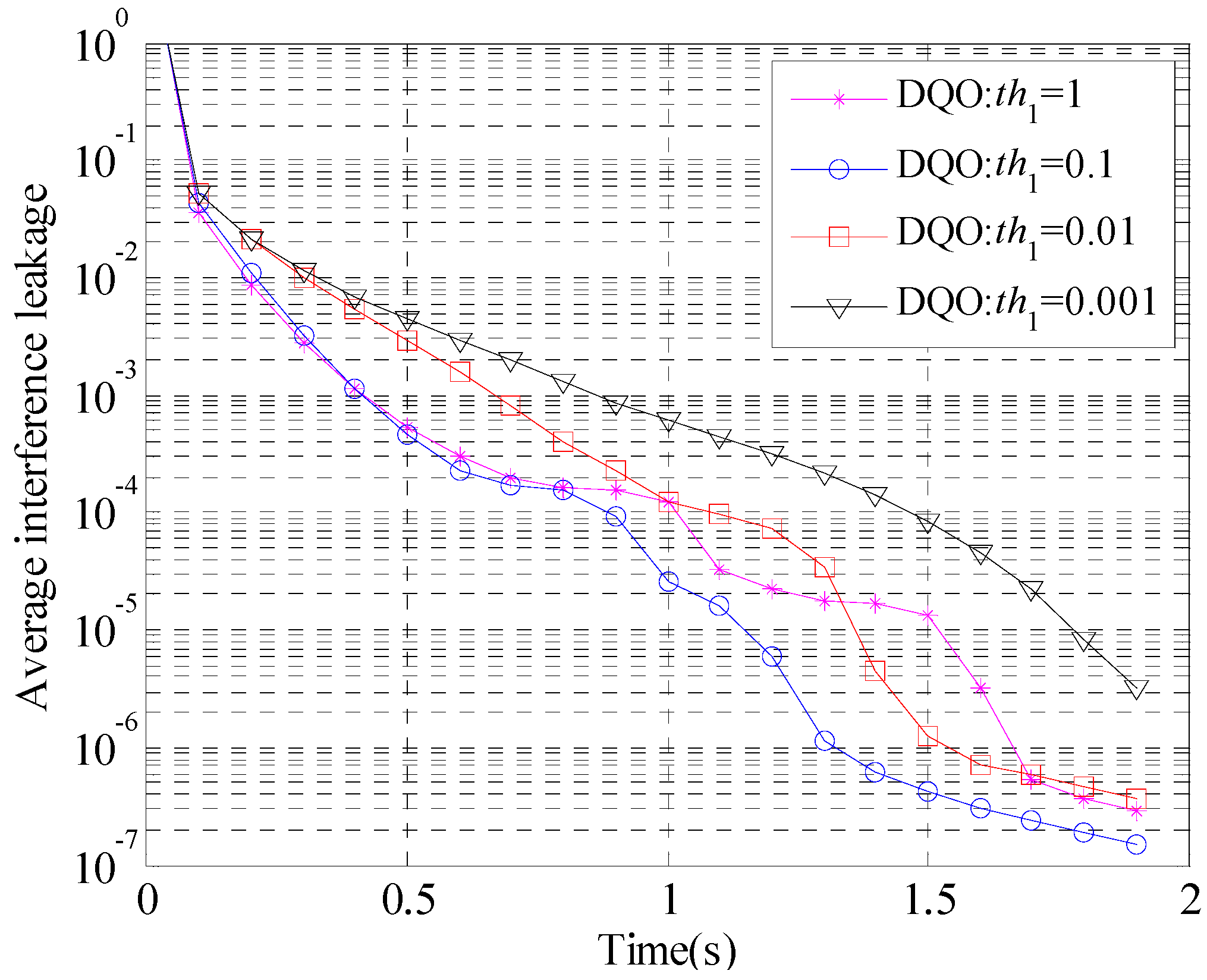
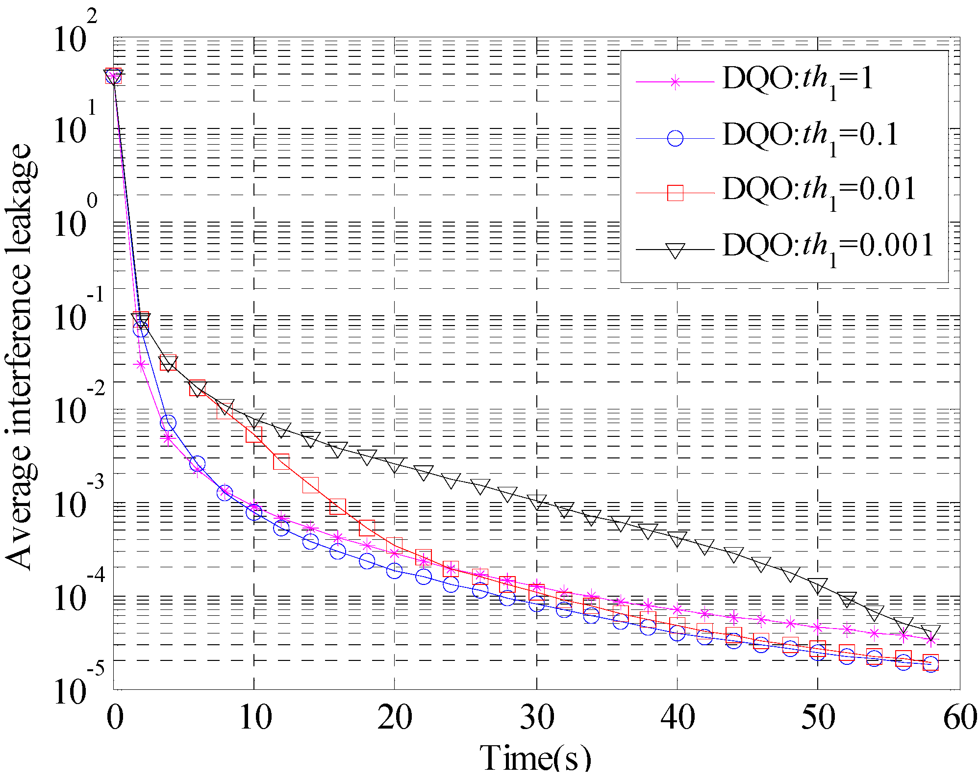
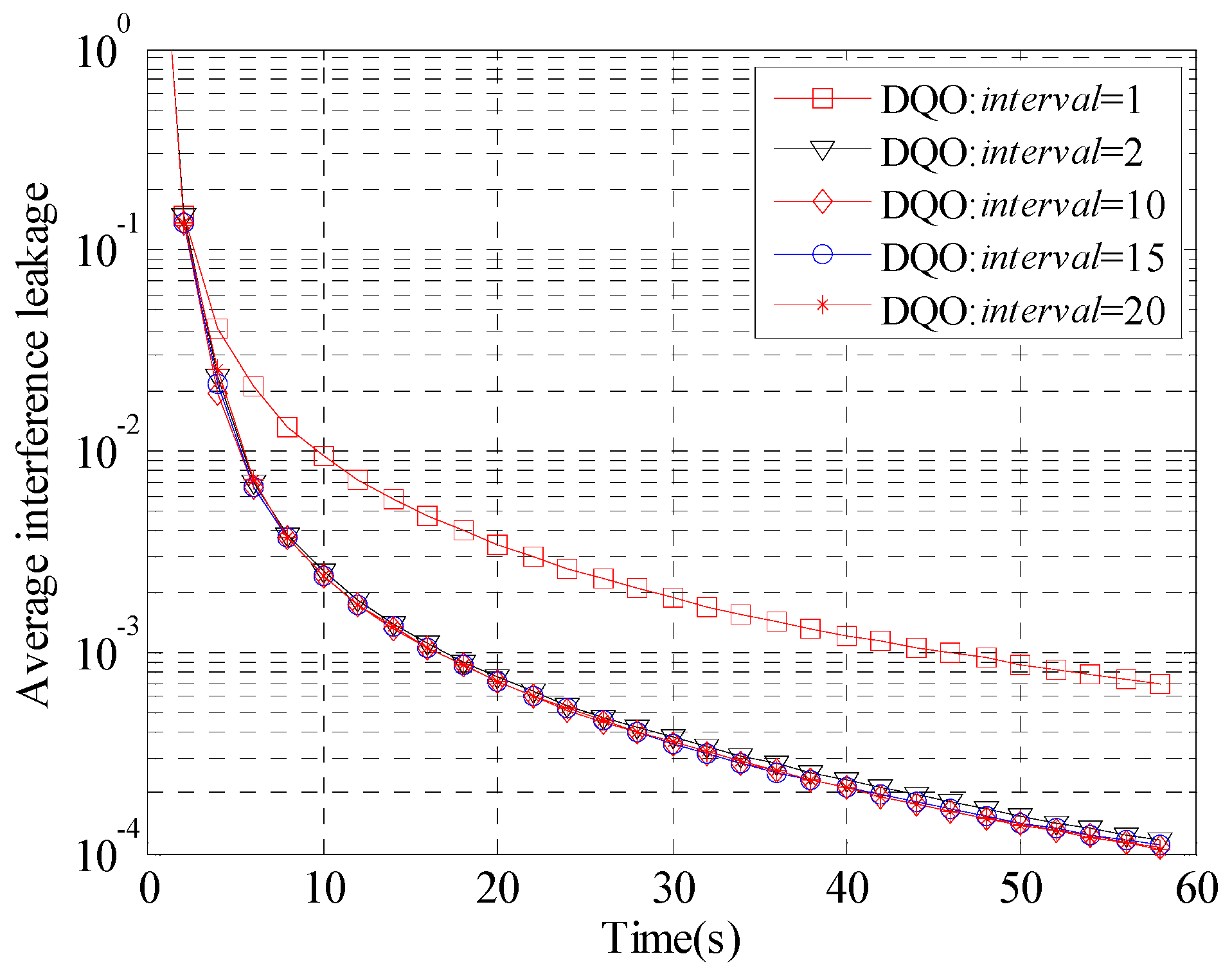
The procedure of DQO algorithm is summarized in Algorithm 2. The framework of DQO algorithm is based on the AMIL algorithm, and the LS procedure is added. In the initial phase of DQO algorithm, it operates just like the AMIL algorithm. The VU and UV steps are executed, and the interference leakage L is evaluated in each iteration. When L is smaller than the preset threshold th₁, as shown in the 21-th line of Algorithm 2, the variable flag is set and the current number of iterations is recorded as i_b, indicating that the current point is close enough to the convergence value and the LS procedure can be implemented. Notice that flag and i_b are updated only once and will remain unchanged afterward. After flag is set, the algorithm will execute the LS procedure every interval iterations, as shown in the 10-th line. The LS procedure cannot be carried out in every iteration for the reason that the approximations Equations (46) and (47) can be attained only when i₁ is large enough.

Algorithm 2 DQO Algorithm

Initialize $V_k^0$, with ${(V_k^0)}^{\text{H}}{V}_k^0=I$ (k = 1, 2,…, K). Initialize parameters: th1, th2 (th2 < th1), Imax, and interval. Set flag = 0, i = 0, and ib = 0. Repeat i = i + 1. (VU-step):Calculate $Q_k^i$ according to Equation (2). Update $U_k^i$ so that $U_{k(l)}^i={\text{eig}}_l[Q_k^i],l=1,2,\mathrm{..},d.$ (UV-step):Calculate $\overleftarrow{Q_k^i}$ according to Equation (3). Update $V_k^i$ so that $V_{k(l)}^i={\text{eig}}_l[\overleftarrow{Q_k^i}],l=1,2,\mathrm{..},d.$ If flag = 1 and (i − ib) mod interval = 0, execute the LS procedure as: (a) Calculate the new iteration direction as: $\Delta U_k=U_k^i-U_k^{i-1}$ $\Delta V_k=V_k^i-V_k^{i-1}$ (b) Calculate the optimal step size t*. (c) Update $V_k^i$ and $U_k^i$ as: $U_k^i\leftarrow U_k^i\text{+}{t}^{*}\Delta U_k$ $V_k^i\leftarrow V_k^i\text{+}{t}^{*}\Delta V_k$ (d) Normalize each column of $V_k^i$ and $U_k^i$. else Calculate the interference leakage L according to Equation (5) If th2 < L < th1 and flag =0 Set flag = 1 and ib = i. end if. end if. Until L < th2 or i > Imax.

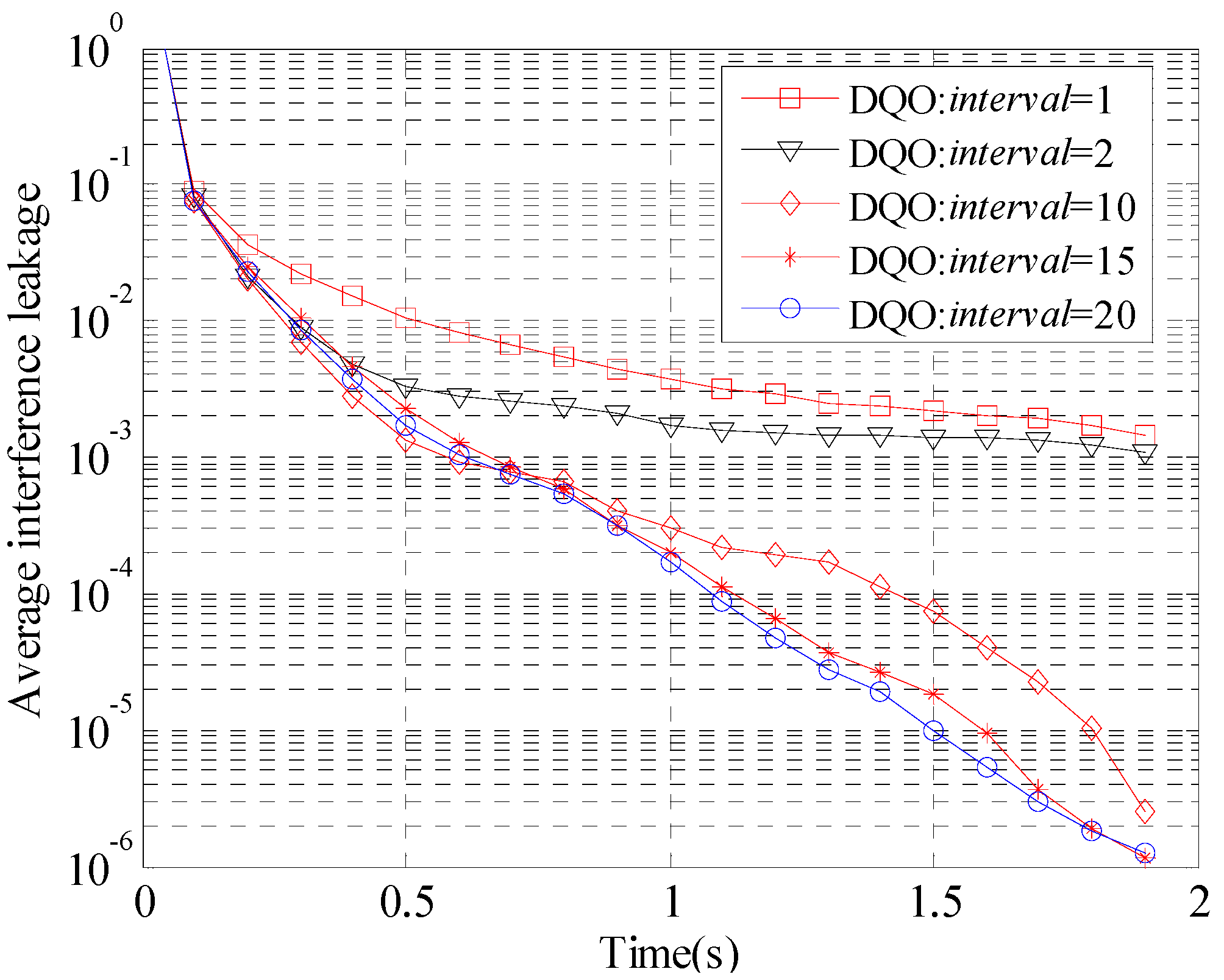
Therefore, it has to take several UV and VU steps before ${\kappa }_1^{i_1}$ takes the dominant proposition so that Equations (35) and (36) hold. As a result, the parameter interval cannot be set to be one, and it will be further validated by simulation in Section 5.1. During each LS procedure, the new direction is calculated by subtracting the consecutive iteration results. The optimal step size t^* can be obtained by solving a quartic optimization problem, and the associated details will be provided in Section 4.2. The new precoders and decoders are updated as the 16-th and 17-th lines. To guarantee the unit norm of the precoders and decoders, we normalize each column of U and V in the 18-th line. The algorithm will stop when the interference leakage is smaller than the objective threshold th₂ or the maximal iterations number I_max is reached.

4.2. Optimal Step Size Calculation

The step size in DQO algorithm is an essential parameter which has a significant impact on the efficiency. Aiming at minimizing the interference leakage along the line search direction, the optimal step size can be calculated analytically by solving a quartic optimization problem. As is shown in Equations (35) and (36), the step size t should be a real value. From Equations (2), (4) and (5), the total interference leakage in the case of U_k + tΔU_k, V_k + tΔV_k (k = 1, 2, …, K) can be formulated as:

$$L(t)={\displaystyle \sum _{k=1}^K{\displaystyle \sum _{l=1,l\ne k}^K\frac{P_l}{d}}}\text{Tr}[(U_k^{\text{H}}+t\mathrm{\Delta }{U}_k^{\text{H}})H_{kl}(V_l+t\mathrm{\Delta }{V}_l)(V_l^{\text{H}}+t\mathrm{\Delta }{V}_l^{\text{H}})H_{kl}^{\text{H}}(U_k+t\mathrm{\Delta }{U}_k)]$$

(54)

Without loss of generality, we assume P_l/d = 1 and define:

$${\alpha }_{kl}=\mathrm{\Delta }{U}_k^{\text{H}}{H}_{kl}{V}_l$$

(55)

$${\beta }_{kl}=\mathrm{\Delta }{U}_k^{\text{H}}{H}_{kl}\mathrm{\Delta }{V}_l$$

(56)

$${\gamma }_{kl}=U_k^{\text{H}}{H}_{kl}\mathrm{\Delta }{V}_l$$

(57)

$${\delta }_{kl}=U_k^{\text{H}}{H}_{kl}{V}_l$$

(58)

Then Equation (54) can be formulated as a real quartic function of t:

$$L(t)=a_4{t}^4+a_3{t}^3+a_2{t}^2+a_1{t}^1+a_0$$

(59)

where:

$$a_4={\displaystyle \sum _{k=1}^K{\displaystyle \sum _{l=1,l\ne k}^K\text{Tr}[{\beta }_{kl}{\beta }_{kl}^{\text{H}}]}}$$

(60)

$$a_3={\displaystyle \sum _{k=1}^K{\displaystyle \sum _{l=1,l\ne k}^{K}2\text{Re}\{\text{Tr}[{\alpha }_{kl}{\beta }_{kl}^{\text{H}}+{\gamma }_{kl}{\beta }_{kl}^{\text{H}}]\}}}$$

(61)

$$a_2={\displaystyle \sum _{k=1}^K{\displaystyle \sum _{l=1,l\ne k}^K\{\text{Tr}[{\alpha }_{kl}{\alpha }_{kl}^{\text{H}}+{\gamma }_{kl}{\gamma }_{kl}^{\text{H}}]+2\text{Re}\{\text{Tr}[{\alpha }_{kl}{\gamma }_{kl}^{\text{H}}+{\beta }_{kl}{\delta }_{kl}^{\text{H}}]\left\}\right\}}}$$

(62)

$$a_1={\displaystyle \sum _{k=1}^K{\displaystyle \sum _{l=1,l\ne k}^{K}2}\text{Re}\{\text{Tr}[{\delta }_{kl}{\alpha }_{kl}^{\text{H}}+{\delta }_{kl}{\gamma }_{kl}^{\text{H}}]\}}$$

(63)

$$a_0={\displaystyle \sum _{k=1}^K{\displaystyle \sum _{l=1,l\ne k}^K\text{Tr}[{\delta }_{kl}{\delta }_{kl}^{\text{H}}]}}$$

(64)

In order to obtain the global minimum value of Equation (59), the following lemma is firstly introduced:

Lemma 1.

For a real quartic function f(t) = a₄t⁴ + a₃t³ + a₂t² + a₁t + a₀, t ∈ R, with a₄ > 0, there exists an optimal t^* ∈ R that satisfies f′(t^*) = 0, so that f(t^*) is the global minimal value of f(t).

Proof of Lemma 1.

As a₄ > 0 and $f^{\prime }(t)=4a_4{t}^3+3a_3{t}^2+2a_{2}t+a_1$, it can be obtained that $\underset{t\to +\infty }{\lim }{f}^{\prime }(t)=+\infty$ and$\underset{t\to -\infty }{\lim }{f}^{\prime }(t)=-\infty$. Therefore, there exist a, b ∈ R, so that f′(t) > 0, t ∈ [b, ∞) and f′(t) < 0, t ∈ (−∞ ,a]. Thus, f(t) increases monotonously in t ∈ [b, ∞) and has the minimal value f(b) at t = b. Similarly, f(t) decreases monotonously in t ∈ (−∞ ,a] and has the minimal value f(a) at t = a. When t ∈ [a, b], due to continuity, f(t) must have the minimal value f(c) at t = c where c ∈ [a, b]. Hence, min{f(a), f(b), f(c)} is the global minimum of f(t). In conclusion, there exists t^* ∈ R (or t^* ∈ {a, b, c}) so that f(t^*) is the global minimal value. For f(t) ≥ f(t^*), the left and right derivatives at t^* can be formulated as:

$$f_{-}^{\prime }(t^{*})=\underset{\mathrm{\Delta }t\to 0^{-}}{\lim }\frac{f(t^{*}+\mathrm{\Delta }t)-f(t^{*})}{\mathrm{\Delta }t}\le 0$$

$$f_{+}^{\prime }(t^{*})=\underset{\mathrm{\Delta }t\to 0^{+}}{\lim }\frac{f(t^{*}+\mathrm{\Delta }t)-f(t^{*})}{\mathrm{\Delta }t}\ge 0$$

For $f^{\prime }(t^{*})=f_{-}^{\prime }(t^{*})=f_{+}^{\prime }(t^{*})$, we must have $f^{\prime }(t^{*})=f_{-}^{\prime }(t^{*})=f_{+}^{\prime }(t^{*})=0$. Therefore, the global optimal value t^* must be chosen from the solutions that satisfy f′(t^*) = 0. When f′(t^*) = 0 has only one real solution, it is the optimal t^*. When f′(t^*) = 0 has 2 or 3 real solutions, t^* is the one that has the smallest function value.

From Equation (60) we have a₄ > 0. According to Lemma 1, it can be deduced that there exists t^* ∈ R with zero derivative, which makes L(t^*) as the global minimal value of Equation (59). Let:

$$dL/dt=4a_4{t}^3+3a_3{t}^2+2a_{2}t+a_1=0$$

(65)

The discriminant of Equation (65) is: $\mathrm{\Delta }={\mathrm{\Delta }}_1^2+{\mathrm{\Delta }}_2^3$, where Δ₁ = (bc)/(6a²) − b³/(27a³) − d/(2a), Δ₂ = c/(3a) − b²/(9a²), a = 4a₄, b = 3a₃, c = 2a₂, and d = a₁. And the 3 solutions of Equation (65) are given by:

$$t_{\text{1}}\text{ = }{x}_{\text{1}}\text{+}{x}_{\text{2}}\text{+}{x}_{\text{3}}$$

(66)

$$t_2=x_1+\frac{(-1+\sqrt{3}i)x_2}{2}+\frac{(-1-\sqrt{3}i)x_3}{2}$$

(67)

$$t_3=x_1+\frac{(-1-\sqrt{3}i)x_2}{2}+\frac{(-1+\sqrt{3}i)x_3}{2}$$

(68)

where x₁ = −b/(3a), $x_2=\sqrt[3]{{\mathrm{\Delta }}_1+\sqrt{\mathrm{\Delta }}}$, and $x_3=\sqrt[3]{{\mathrm{\Delta }}_1-\sqrt{\mathrm{\Delta }}}$. When Δ > 0 or Δ = Δ₁ = Δ₂ = 0, there is only one real root t₁ which is the optimal t^*; when Δ = 0 and Δ₁ = Δ₂ ≠ 0, there are 2 real roots; when Δ < 0, there are 3 real roots. If there are more than one real root, t^* is the one that has the smallest function value.

4.3. Computational Complexity Analysis

The computational complexity of the AMIL and DQO algorithms is analyzed according to the number of complex multiplications (NoCM). For the AMIL algorithm, the complexity comes from the covariance matrices calculation, eigenvalue decomposition, and interference leakage evaluation with the complexity of K(K − 1)(MNd + Md² + Nd²), 9K(M³ + N³), and K(K − 1)(d²M + d³), respectively [17]. Therefore the NoCM per iteration of the AMIL algorithm is summarized as:

$$C_{\text{AMIL}}=K(K-1)(2MNd+N{d}^2+M^{2}d)+9K(N^3+M^3)+K(K-1)(d^{2}M+d^3)$$

(69)

For the DQO algorithm, the complexity of the VU-step, UV-step, and interference leakage calculations are the same as those of the AMIL algorithm, and the extra complexity comes from the LS procedure. The complexity of LS comes from the coefficients calculation of Equations (55)–(58) and Equations (60)–(63), solving Equation (65), and normalization. The complexity of each LS procedure is analyzed as follows:

(1) As shown in Equation (55), α_kl can be rewritten as ${\alpha }_{kl}=[{(U_k^i)}^{\text{H}}{H}_{kl}-{(U_k^{i-1})}^{\text{H}}{H}_{kl}]V_l$. Since ${(U_k^i)}^{\text{H}}{H}_{kl}$ and ${(U_k^{i-1})}^{\text{H}}{H}_{kl}$ have been calculated in ${\overleftarrow{Q}}_k$ as shown in Equation (3), the complexity of computing α_kl only comes from the multiplication of $[{(U_k^i)}^{\text{H}}{H}_{kl}-{(U_k^{i-1})}^{\text{H}}{H}_{kl}]$ and $V_l$, with the NoCM of d²M. As k and l traverse from 1 to K with l ≠ k, the total complexity of calculating all α_kl is K(K − 1)d²M. Similarly, β_kl, γ_kl, and δ_kl have the same complexity as α_kl.

(2) The complexity of calculating a₁–a₄ mainly comes from the multiplications among α_kl, β_kl, γ_kl, and δ_kl. Notice that only the traces of the products are required, and we don’t have to compute all the elements of the products. Therefore, the complexity of calculating a₁–a₄ are 2K(K − 1)d², 4K(K − 1)d², 2K(K − 1)d², and K(K − 1)d², respectively. Notice that there is no need to calculate a₀.

(3) The number of real solutions of Equation (65) depends on Δ₁, Δ₂ as well as Δ, and we consider the most complex case of 3 real solutions. The details of the complexity of solving the cubic equation are listed in Table 1. NoRM, NoRD, NoSRC, and NoCRC are employed to represent the number of real multiplications, real divisions, square root calculations, and cubic root calculations, respectively.

Table 1. Complexity of solving the cubic Equation (65).

Types	NoRM	NoRD	NoSRC	NoCRC
a, b, c, d	3	0	0	0
Δ1	9	3	0	0
Δ2	4	2	0	0
Δ	3	0	0	0
x1	1	1	0	0
x2	0	0	1	1
x3	0	0	1	1
t1	0	0	0	0
t2	8	0	0	0
t3	8	0	0	0
L(t)	21	0	0	0
Total	57	6	2	0

Table 1. Complexity of solving the cubic Equation (65).

Types	NoRM	NoRD	NoSRC	NoCRC
a, b, c, d	3	0	0	0
Δ1	9	3	0	0
Δ2	4	2	0	0
Δ	3	0	0	0
x1	1	1	0	0
x2	0	0	1	1
x3	0	0	1	1
t1	0	0	0	0
t2	8	0	0	0
t3	8	0	0	0
L(t)	21	0	0	0
Total	57	6	2	0

(4) $V_k^i$ and $U_k^i$ are normalized so that the norm of each column is one. The normalization of one column of $V_k^i$ takes M complex multiplications, one square root calculation and two real divisions. Therefore the normalization of all the precoding matrices takes dMK complex multiplications, dK square root calculations, and 2dK real divisions. Similarly, the normalization of all the decoding matrices takes dNK complex multiplications, dK square root calculations, and 2dK real divisions.

(5) As the complexity of one complex multiplication equals four real multiplications, the number of real multiplications will be replaced with the equivalent number of complex multiplications. And the complexity of one line search is summarized in Table 2.

Therefore the total number of equivalent complex multiplications of one line search is:

$$C_{\text{LS}}=4K(K-1)d^{2}M+9K(K-1)d^2+dK(M+N)+14.25$$

(70)

And the number of real divisions, square root calculations and cubic root calculations in one LS are 4dK + 6, 2dK + 2, and 2, respectively. As LS is implemented every interval iteration, the average NoCM per iteration of DQO algorithm is:

$$C_{\text{DQO}}=C_{\text{AMIL}}+C_{\text{LS}}/interval$$

(71)

Table 2. Complexity of one line search.

Types	NoRM	NoRD	NoSRC	NoCRC
αkl	K(K − 1)d2M	0	0	0
βkl	K(K − 1)d2M	0	0	0
γkl	K(K − 1)d2M	0	0	0
δkl	K(K − 1)d2M	0	0	0
a1	2K(K − 1)d2	0	0	0
a2	4K(K − 1)d2	0	0	0
a3	2K(K − 1)d2	0	0	0
a4	K(K − 1)d2	0	0	0
Solve (65)	14.25	6	2	2
Normalization	dK(M + N)	4dK	2dK	0

Table 2. Complexity of one line search.

Types	NoRM	NoRD	NoSRC	NoCRC
αkl	K(K − 1)d2M	0	0	0
βkl	K(K − 1)d2M	0	0	0
γkl	K(K − 1)d2M	0	0	0
δkl	K(K − 1)d2M	0	0	0
a1	2K(K − 1)d2	0	0	0
a2	4K(K − 1)d2	0	0	0
a3	2K(K − 1)d2	0	0	0
a4	K(K − 1)d2	0	0	0
Solve (65)	14.25	6	2	2
Normalization	dK(M + N)	4dK	2dK	0

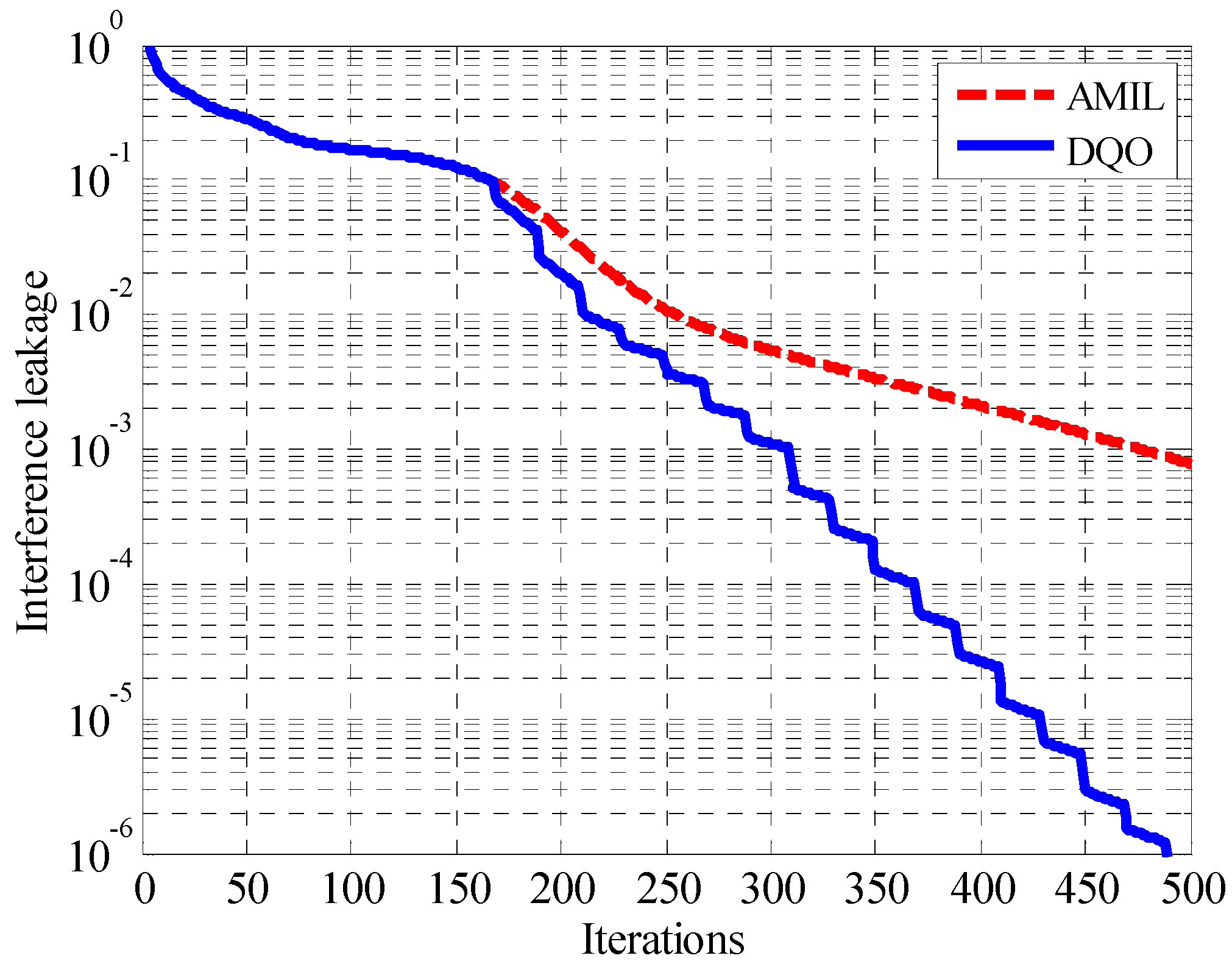
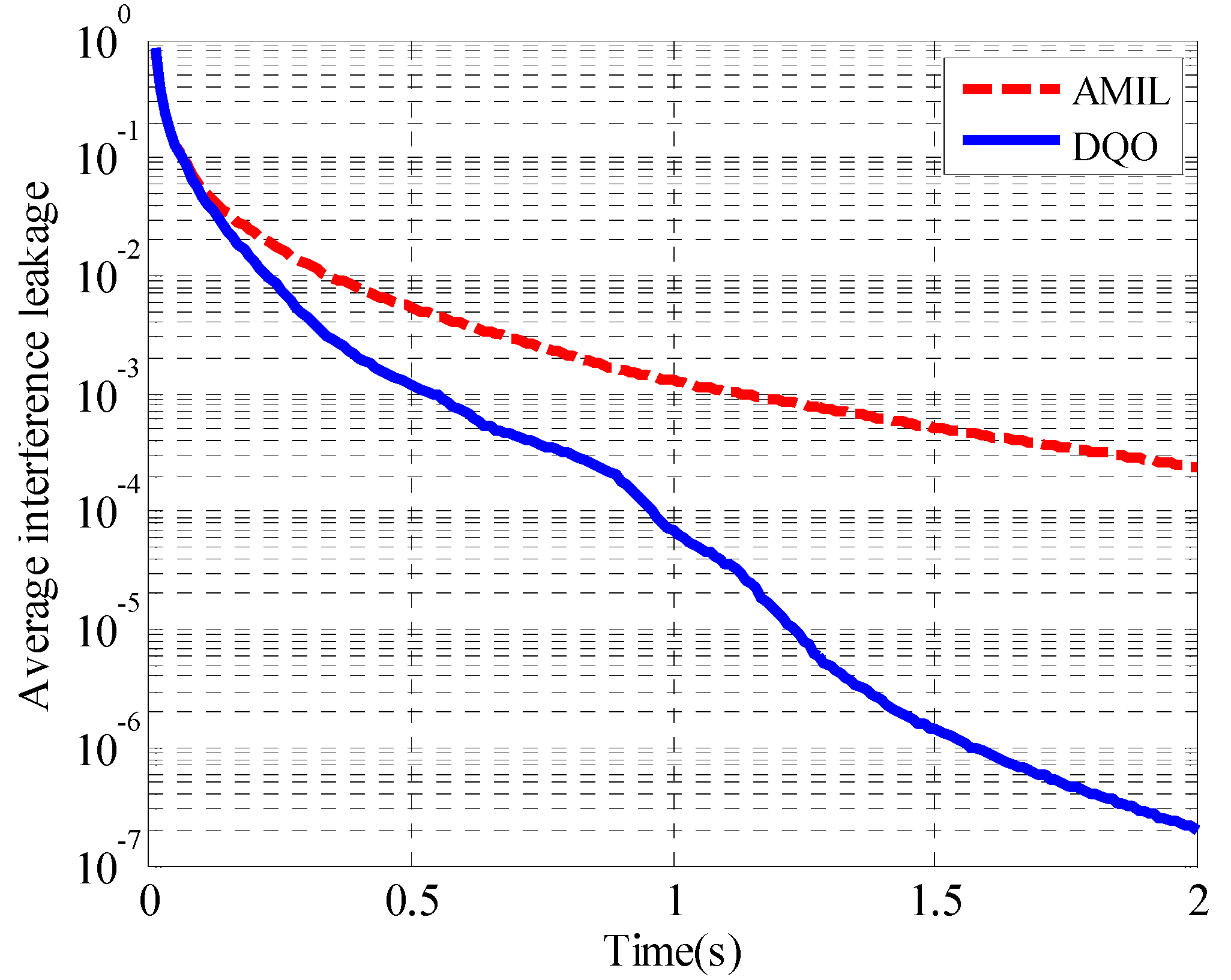
The complexity of the AMIL and DQO algorithms with the parameter interval = 20 (the mechanism for determining the parameter will be provided in Section 5.1) is compared in Table 3. From the comparison, it can be seen that the average NoCM of the DQO algorithm per iteration is only slightly higher than that of the AMIL algorithm. Although LS will bring extra complexity per iteration, it can reduce the number of iterations significantly and thus lower the overall computational complexity, which will be shown in the numerical results.

Table 3. Complexity of AMIL and DQO algorithms in (M × M, d)^K with interval = 20.

(M × N, d)K	CAMIL	CDQO	CDQO/CAMIL
(6 × 6, 1)11	5.61 × 104	5.63 × 104	1.003
(6 × 6, 2)5	2.49 × 104	2.50 × 104	1.006
(7 × 7, 1)13	1.06 × 105	1.06 × 105	1.003
(7 × 7, 2)6	4.78 × 104	4.80 × 104	1.005
(8 × 8, 1)15	1.82 × 105	1.83 × 105	1.002
(8 × 8, 2)7	8.37 × 104	8.40 × 104	1.004
(9 × 9, 1)17	2.94 × 105	2.95 × 105	1.002
(9 × 9, 2)8	1.37 × 105	1.37 × 105	1.004
(10 × 10, 1)19	4.52 × 105	4.53 × 105	1.002
(10 × 10, 2)9	2.12 × 105	2.12 × 105	1.003

Table 3. Complexity of AMIL and DQO algorithms in (M × M, d)^K with interval = 20.

(M × N, d)K	CAMIL	CDQO	CDQO/CAMIL
(6 × 6, 1)11	5.61 × 104	5.63 × 104	1.003
(6 × 6, 2)5	2.49 × 104	2.50 × 104	1.006
(7 × 7, 1)13	1.06 × 105	1.06 × 105	1.003
(7 × 7, 2)6	4.78 × 104	4.80 × 104	1.005
(8 × 8, 1)15	1.82 × 105	1.83 × 105	1.002
(8 × 8, 2)7	8.37 × 104	8.40 × 104	1.004
(9 × 9, 1)17	2.94 × 105	2.95 × 105	1.002
(9 × 9, 2)8	1.37 × 105	1.37 × 105	1.004
(10 × 10, 1)19	4.52 × 105	4.53 × 105	1.002
(10 × 10, 2)9	2.12 × 105	2.12 × 105	1.003

5. Numerical Results

In this section, the performance of the proposed DQO algorithm is evaluated and compared with the traditional AMIL algorithm by simulation. We will employ the interference leakage and sum rate as the performance metrics. The definition of interference leakage is shown in Equation (5), and that of sum rate can be found in reference [23]. Unless specially specified, 250 realizations of different channel coefficients with distribution CN(0, 1) and the corresponding initial precoding matrices are randomly generated to evaluate the average interference leakage and sum rate of the algorithms in each simulation.

5.1. Parameter Analysis

There are four parameters in the DQO algorithm: the interference leakage threshold for starting LS th₁, the desired interference leakage th₂, the interval for executing the LS interval, and the maximum iteration I_m. The parameters th₂ and I_m are set according to the practical requirements. The other two have impacts on the efficiency of DQO algorithm. It is difficult to provide the exact optimal values of the two parameters analytically. Therefore, simulations are employed to determine the parameters th₁ and interval in this section.

The parameter th₁ decides the interference leakage threshold for starting line search. It is difficult to provide the exact optimal value of th₁, and the performance of DQO algorithm is evaluated with different th₁ for the (5 × 5, 2)⁴ and (10 × 10, 1)¹⁹ channels in Figure 2 and Figure 3, respectively. The parameter interval is preseted as 20, and th₁ is chosen to be 1, 0.1, 0.01, and 0.001.

Figure 2. Convergence curves of the average interference leakage of DQO algorithm with th₁ = 1, 0.1, 0.01, and 0.001 in (5 × 5, 2)⁴.

Figure 2. Convergence curves of the average interference leakage of DQO algorithm with th₁ = 1, 0.1, 0.01, and 0.001 in (5 × 5, 2)⁴.

As is shown in Theorem 2, the difference between the two consecutive iteration results of AMIL algorithm will approximately point to the convergence solution when the current precoding and decoding matrices are sufficiently close to their convergence values. In DQO algorithm, the interference leakage is employed to be a measure of the distance between the current point and the convergence point, and line search is started when the interference leakage is smaller than a preseted threshold th₁. If th₁ is set to be too large, the generated direction does not point to the convergence value. If th₁ is set to be too small, the line search procedure cannot accelerate the convergence rate in time, and the effectiveness of DQO algorithm is degraded.

As is shown in Figure 2 and Figure 3, th₁ = 0.1 has better performance than the too large value 1 and the too small value 0.001, which accords with the analysis above. Therefore, the parameter th₁ is set to be 0.1 in the following simulations.

Figure 3. Convergence curves of the average interference leakage of DQO algorithm with th₁ = 1, 0.1, 0.01, and 0.001 in (10 × 10, 1)¹⁹.

Figure 3. Convergence curves of the average interference leakage of DQO algorithm with th₁ = 1, 0.1, 0.01, and 0.001 in (10 × 10, 1)¹⁹.

The parameter interval controls the frequency of executing line search. The parameter cannot be set to be too small. This can be explained by the fact that Equations (46) and (47) can be attained only when i₁ in Equation (45) is large enough. Therefore, it has to take several UV and VU steps before ${\kappa }_1^{i_1}$ in Equation (45) takes the dominant proposition so that Equations (35) and (36) hold.

The performance of DQO algorithm with different interval for the (5 × 5, 2)⁴ and (10 × 10, 1)¹⁹ channels is evaluated in Figure 4 and Figure 5, respectively. The parameter th₁ is preseted as 0.1, and interval is chosen to be 1, 2, 10, 15, and 20. The curves with interval = 1 converge slowly, which verifies the analysis above. On the other hand, when interval is large enough, the convergence curves are very close to each other. As interval = 20 has better performance than the others in Figure 4, interval is chosen to be 20 in the following simulations.

Figure 4. Convergence curves of the average interference leakage of DQO algorithm with interval = 1, 2, 10, 15, and 20 in (5 × 5, 2)⁴.

Figure 4. Convergence curves of the average interference leakage of DQO algorithm with interval = 1, 2, 10, 15, and 20 in (5 × 5, 2)⁴.

Figure 5. Convergence curves of the average interference leakage of DQO algorithm with interval = 1, 2, 10, 15, and 20 in (10 × 10, 1)¹⁹.

Figure 5. Convergence curves of the average interference leakage of DQO algorithm with interval = 1, 2, 10, 15, and 20 in (10 × 10, 1)¹⁹.

5.2. Comparison of Different Algorithms

In this subsection, the performance of the DQO and AMIL algorithms is compared and analyzed. The parameters for the DQO algorithm are set as th₁ = 0.1 and interval = 20. The interference leakage with respective to iterations for one realization of randomly generated channel coefficients in the (5 × 5, 2)⁴ channel is shown in Figure 6, which provides us the overall effectiveness of DQO algorithm. As reflected in the figure, the interference leakage of the two algorithms remains the same before 168 iterations since they employ the same VU and UV steps. When the interference leakage is smaller than threshold th₁, DQO algorithm begins to perform the LS procedure, and a step-like decrease in interference leakage can be observed. After 350 iterations, DQO algorithm reaches the interference leakage of 1.2 × 10⁻⁴, which is one order lower than that of AMIL algorithm. The difference of the interference leakage becomes larger as the iterations increase, and DQO algorithm can reach the level which is 3 orders lower than that of AMIL algorithm. Therefore, the DQO algorithm can reach the same level of interference leakage as the traditional AMIL method with much fewer iterations.

Figure 6. Convergence curves of the interference leakage for one realization of randomly generated channel coefficients in (5 × 5, 2)⁴.

Figure 6. Convergence curves of the interference leakage for one realization of randomly generated channel coefficients in (5 × 5, 2)⁴.

As iterations cannot represent the complexity of the two algorithms sufficiently, the average performance of the two algorithms is evaluated in terms of execution time in the following simulations. Average interference leakage as well as sum rate in (5 × 5, 2)⁴ and (10 × 10, 1)¹⁹ channels are considered. The convergence of average interference leakage for (5 × 5, 2)⁴ channel is illustrated in Figure 7.

Figure 7. Convergence curves of the average interference leakage in (5 × 5, 2)⁴.

Figure 7. Convergence curves of the average interference leakage in (5 × 5, 2)⁴.

From the results, it can be seen that the DQO algorithm can suppress the interference leakage to 6.8 × 10⁻⁵ while the AMIL algorithm can only reach the level of 1.2 × 10⁻³ at 1 s. The difference of the average interference leakage between them increases with time, and the DQO algorithm outperforms the AMIL algorithm with three orders lower at 2 s. The convergence of the average sum rate with SNR = 40 dB for (5 × 5, 2)⁴ channel is depicted in Figure 8.

Figure 8. Convergence curves of the average sum rate in (5 × 5, 2)⁴.

Figure 8. Convergence curves of the average sum rate in (5 × 5, 2)⁴.

As reflected in the figure, the average sum rate of the DQO algorithm increases more rapidly than that of the AMIL algorithm during the first 0.5 s and the DQO algorithm converges approximately at 0.61 s with the average sum rate of 104 bps/Hz while the AMIL algorithm takes about 1.78 s to reach the same level. Like the (5 × 5, 2)⁴ case, the convergence curves of average interference leakage as well as sum rate for (10 × 10, 1)¹⁹ channel are plotted in Figure 9 and Figure 10, respectively. As the number of users and antennas has become larger, it requires more iterations as well as computational time to suppress the interference leakage and to increase the sum rate. In Figure 9, the DQO algorithm can suppress the interference leakage more rapidly than the AMIL algorithm and achieves the interference leakage of 5.6 × 10⁻⁵ at 60 s, which is one order lower than that of the AMIL algorithm. In particular, the AMIL algorithm seems to converge at approximately 60 s while the DQO algorithm has the tendency to reach an even lower level of interference leakage afterward. In Figure 10, the average sum rate of the DQO algorithm converges much more rapidly than that of the AMIL algorithm during the first 10 s and the DQO algorithm achieves a higher average sum rate than the AMIL algorithm. To further compare their efficiency, average iterations N_AMIL and N_DQO as well as executing time T_AMIL and T_DQO with th₂ = 10⁻⁴ are listed in the cases of different numbers of users and antennas in Table 4. Yetis et al. [32] have provided the feasible condition for IA in the (M × N, d)^K channel as d ≤ (M + N)/(K + 1), therefore we mainly provide the results of the most complex situation when d = (M + N)/(K + 1).

Figure 9. Convergence curves of the average interference leakage in (10 × 10, 1)¹⁹.

Figure 9. Convergence curves of the average interference leakage in (10 × 10, 1)¹⁹.

Figure 10. Convergence curves of the average sum rate in (10 × 10, 1)¹⁹.

Figure 10. Convergence curves of the average sum rate in (10 × 10, 1)¹⁹.

The convergence rate and complexity of the algorithms can be compared by the iterations and computational time which are required to reach a certain level of interference leakage. As is shown in Table 4, the iterations and executing time of the DQO algorithm are only 22%–33% and 23%–33% of those of the AMIL algorithm, respectively. Therefore, simulations above confirm that DQO algorithm can converge faster than the AMIL algorithm and save nearly 2/3 of the computational complexity.

Table 4. Comparison between AMIL and DQO algorithms in (M × N, d)^K.

(M × N, d)K	NAMIL	NDQO	NDQO/NAMIL	TAMIL(s)	TDQO(s)	TAMIL/TDQO
(6 × 6, 1)11	3.38 × 103	7.76 × 102	0.22	17.12	3.89	0.23
(6 × 6, 2)5	2.63 × 103	8.13 × 102	0.31	4.09	1.27	0.31
(7 × 7, 1)13	4.93 × 103	1.27 × 103	0.25	35.75	9.03	0.25
(7 × 7, 2)6	4.60 × 103	1.47 × 103	0.32	9.94	3.18	0.32
(8 × 8, 1)15	7.23 × 103	1.74 × 103	0.24	64.26	15.35	0.24
(8 × 8, 2)7	6.16 × 103	2.06 × 103	0.33	17.75	5.91	0.33
(9 × 9, 1)17	8.35 × 103	2.04 × 103	0.24	99.33	24.16	0.24
(9 × 9, 2)8	8.12 × 103	2.24 × 103	0.27	30.61	8.41	0.27
(10 × 10, 1)19	9.44 × 103	2.52 × 103	0.27	140.12	36.71	0.27
(10 × 10, 2)9	8.94 × 103	2.35 × 103	0.26	42.49	11.10	0.26

Table 4. Comparison between AMIL and DQO algorithms in (M × N, d)^K.

(M × N, d)K	NAMIL	NDQO	NDQO/NAMIL	TAMIL(s)	TDQO(s)	TAMIL/TDQO
(6 × 6, 1)11	3.38 × 103	7.76 × 102	0.22	17.12	3.89	0.23
(6 × 6, 2)5	2.63 × 103	8.13 × 102	0.31	4.09	1.27	0.31
(7 × 7, 1)13	4.93 × 103	1.27 × 103	0.25	35.75	9.03	0.25
(7 × 7, 2)6	4.60 × 103	1.47 × 103	0.32	9.94	3.18	0.32
(8 × 8, 1)15	7.23 × 103	1.74 × 103	0.24	64.26	15.35	0.24
(8 × 8, 2)7	6.16 × 103	2.06 × 103	0.33	17.75	5.91	0.33
(9 × 9, 1)17	8.35 × 103	2.04 × 103	0.24	99.33	24.16	0.24
(9 × 9, 2)8	8.12 × 103	2.24 × 103	0.27	30.61	8.41	0.27
(10 × 10, 1)19	9.44 × 103	2.52 × 103	0.27	140.12	36.71	0.27
(10 × 10, 2)9	8.94 × 103	2.35 × 103	0.26	42.49	11.10	0.26

6. Conclusions and Future Work

In this paper, the properties of the traditional AMIL algorithm for IA have been studied. It has been found that if the AMIL algorithm can converge to a point where the interference leakage is very small, there exist fixed linear transformations T_V and T_U that exert on the deviations when the current point is sufficiently close to the convergence value. Particularly, successive exertions of the transformations on the deviations will lead to an interesting property that the difference of the consecutive iterations of AMIL algorithm will approximately point to the convergence value. Based on this discovery, a rapid convergent low-complexity minimization interference leakage algorithm, namely the DQO algorithm, has been proposed to speed up the convergence rate by employing optimal line search procedure. The direction for LS is generated by subtracting the consecutive iteration results of the AMIL algorithm, and the optimal step size can be determined analytically by optimizing a quartic function. Complexity analysis of the DQO and AMIL algorithms has been provided, and simulation results have shown that the DQO algorithm can reduce the number of iterations and execution time significantly under the same interference leakage and sum rate conditions. In the future, we will focus on extending the proposed algorithm to many more scenarios, such as systems with imperfect CSI [33,34], cooperative communications [35], and so on.