1. Introduction
Shafts are one of most important machine elements and the accuracy of machined shafts has a significant effect on the properties of any mechanical device that employs one. The accuracy of a machined shaft can be ensured using a Computer Numerical Control lathe, but mechanical wear in a CNC lathe system, system deformation, and the radial wear of the machining tools will reduce the accuracy of the machined shaft. If the variation of the shaft diameter could be monitored during its machining, the dimensional accuracy of the product could be ensured by the automatic compensation system of the CNC lathe. Therefore, on-line measurement of shaft size is very important in machining.
A variety of noncontact machine vision methods for measuring the product diameters have been proposed [
1,
2,
3,
4,
5]. These methods can be classified as active methods and passive methods. Passive measurement methods use a camera or two cameras to obtain shaft diameters [
6,
7]. In 2008, Song
et al. [
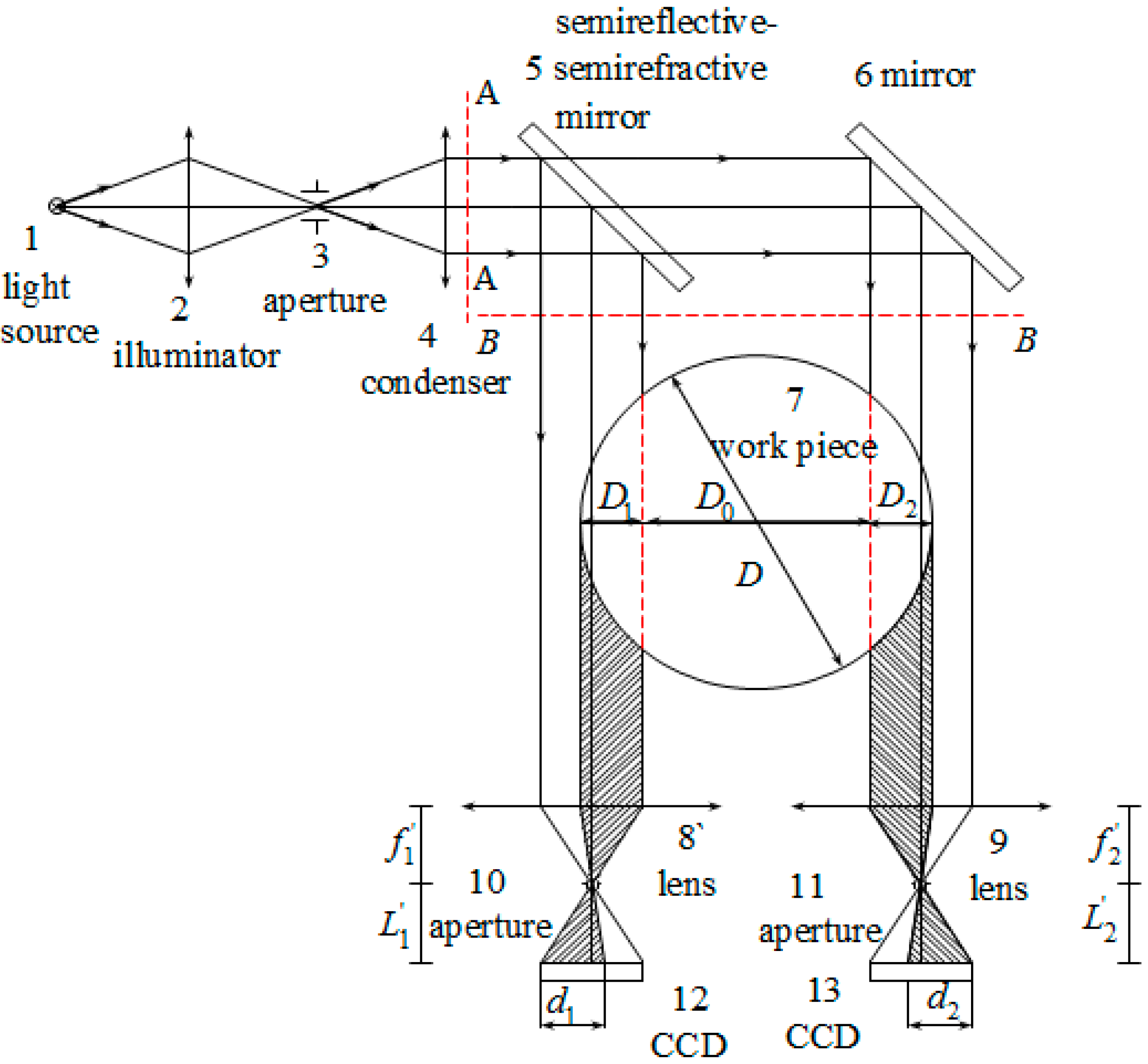
8] proposed a method where both edges of a shaft were imaged onto two cameras through two parallel light paths as shown in
Figure 1 [
8]. Using this approach, the shaft diameter was obtained by measuring the length of the photosensitive units on the shadow field of the two CCDs (Charge-Coupled Device) and the distance between the two parallel light paths. This method can amplify the measurement range while ensuring the measuring accuracy; however, it is very difficult to calibrate the position of the two cameras.
Figure 1.
The optical principle of the parallel light projection method with double light paths (with permission from [
8]).
Figure 1.
The optical principle of the parallel light projection method with double light paths (with permission from [
8]).
In 2013, Sun [
9] used a camera to obtain shaft diameters, employing a theory of plane geometry in the cross-section, which is perpendicular to the axis of the shaft, as shown in
Figure 2 [
9]. This method can achieve a high measuring accuracy, but it requires the calibration of the plane of the center line of the shaft before the measurement. In practice, the position of the center line changes each time the shaft is clamped by the jaw chucks of the lathe. This change of position will decrease the accuracy of measurement.
Figure 2.
The orientations of the shaft and the measurement plane in 3D space (with permission from [
9]).
Figure 2.
The orientations of the shaft and the measurement plane in 3D space (with permission from [
9]).
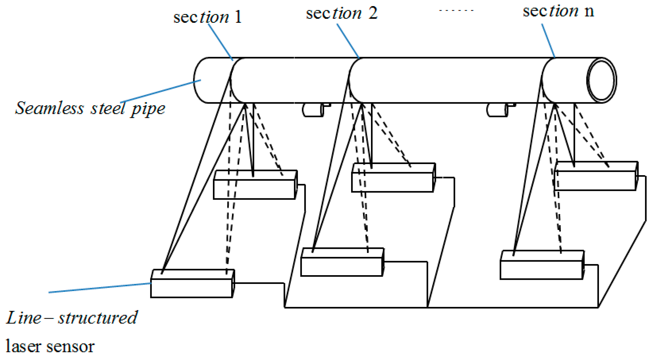
Active measurement methods generally use one or more cameras and lasers to achieve accurate measurements of shaft diameters. In 2001, Sun
et al. [
10] used a pair of line-structured lasers and cameras to measure shaft diameters, as shown in
Figure 3 [
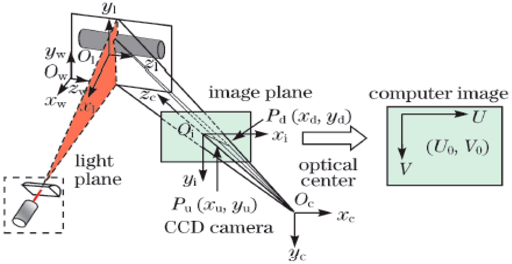
10]. The lights was projected onto the pipe, then captured by two cameras, and the diameter of a steel pipe could be determined by fitting the ellipse with the two developed arcs. It is difficult to ensure that the two arcs are on the same plane, so the accuracy of the method is limited. In 2010, Liu
et al. [
11] reported a method for measuring shaft diameters using a line-structured laser and a camera, as shown in
Figure 4 [
11]. The coordinates of the light stripe projected on the shaft were obtained using a novel gray scale barycenter extraction algorithm along the radial direction. The shaft diameter was then obtained by circle fitting using the generated coordinates. If the line-structured light is perpendicular to the measured shaft, the shaft diameter can be obtained by fitting a circle. Thus, this method is limited by the measurement environment.
Figure 3.
Sketch of the measurement system (with permission from [
10]).
Figure 3.
Sketch of the measurement system (with permission from [
10]).
Figure 4.
Mathematical model of the system (with permission from [
11]).
Figure 4.
Mathematical model of the system (with permission from [
11]).
In this study, a method for measuring shaft diameter is proposed using a line-structured laser and a camera. Based on the direction vector of the measured shaft axis, which is calibrated before the measurement, a virtual plane is established perpendicular to the axis and the image of a light stripe on the shaft is projected to the virtual plane. The shaft diameter is then determined from the projected image on the virtual plane. To improve the measuring precision, the center of the projected image was determined by fitting the projected image using a set of geometrical constraints.
This report is organized as follows:
Section 2 calibrates the structured light system.
Section 3 outlines the model of the proposed method.
Section 4 reports the experimental results used to test the measuring accuracy and influences of several factors.
Section 5 provides the study’s conclusions.
3. The Principle and Model of the Measurement
The model for measuring the shaft diameters is shown in
Figure 6. A shaft is clamped at two centers, images of the shaft are captured by a CCD camera, п1 is the light plane, and
MN is the axis of the shaft. The stripe
ab is formed by projecting the light plane п1 onto the measured shaft. The pixel coordinates
of
ab stripe centers are extracted by Steger’s algorithm. The virtual plane п
2 perpendicular to the measured shaft is created and the normal vector of п
2 is the directional vector of the axis
MN. Although the position of the axis changes slightly every time a shaft is clamped, the direction of the axis does not change. Thus, the equation of the virtual plane п
2 can be obtained in O
CX
CY
CZ
C (see
Appendix A for the details):
The arc cd is formed by the virtual plane п2 intersecting the measured shaft.
Figure 6.
The measurement model of the shaft. (a) global view, (b) local view.
Figure 6.
The measurement model of the shaft. (a) global view, (b) local view.
Since the light plane п
1 is not perpendicular to the shaft, the cross-section is an ellipse and the shaft diameter can be obtained by fitting the ellipse with stripe centers
Pi. The elliptic equation is:
The parameters of Equation (10) can be obtained by the least squares method, and the length of the minor axis d is the measured shaft diameter:
Since the virtual plane п
2 is perpendicular to the shaft, the cross-section is a circle and the diameter can be obtained by fitting the circle with points
Qi, which are
Pi projecting on the virtual plane п
2. The circle equation is
The parameters of Equation (12) can be obtained by the least squares method, and the circle diameter d
1 is the measured shaft diameter:
Since the pixel coordinates of the extracted stripe centers have errors, from the numerical analysis, the measuring accuracy of the shaft diameter by circle fitting is better than by ellipse fitting (see
Appendix B for the detail).
The image coordinates
of
Pi can be achieved using Equations (3) and (4), so the equations of
OCPi are:
The camera coordinates
can be obtained using Equations (5) and (14):
A set of lines
PiQi are made by passing through the extracted centers
and parallel to the measured shaft axis, as shown in
Figure 6b. Since the axis
MN is perpendicular to the plane п
2, the direction vectors of the lines are the normal vector of п
2,
. Thus, the equations of lines
PiQi are:
Each line PiQi has an intersection point Qi on the plane п2. The camera coordinates of the intersection points are obtained using Equations (9) and (16), respectively.
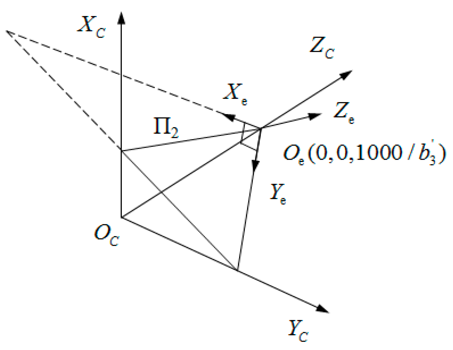
Figure 7.
Oe—XeYeZe and OC—XCYCZC.
Figure 7.
Oe—XeYeZe and OC—XCYCZC.
To facilitate the circle fitting, a coordinate system (O
e—X
eY
eZ
e) is established on the plane п
2, as shown in
Figure 7. In O
e—X
eY
eZ
e, X
eY
e plane is the plane п
2, O
eZ
e axis is perpendicular to the plane п
2, and the origin of coordinate O
e is the intersection point of the plane п
2 with O
CZ
C axis. Additionally, camera coordinates of the origin of O
e can be obtained by Equation (9). Thus, translations of the camera coordinate system are
relative to O
e—X
eY
eZ
e and the camera coordinate Q
i can be changed into O
e—X
eY
eZ
e by Equation (17):
where,
is the rotation angle round O
CY
C,
is the rotation angle round O
CX
C, and
are the coordinates of
in O
e—X
eY
eZ
e.
Normal vector
of the plane п
2 is converted by the coordinate rotation into
in O
e-X
eY
eZ
e, where,
. Thus,
values before and after the conversion are substituted into Equation (18):
and
are obtained by Equation (18). In O
e-X
eY
eZ
e, because points
Qi are on п
2, the coordinates
Qi are
.
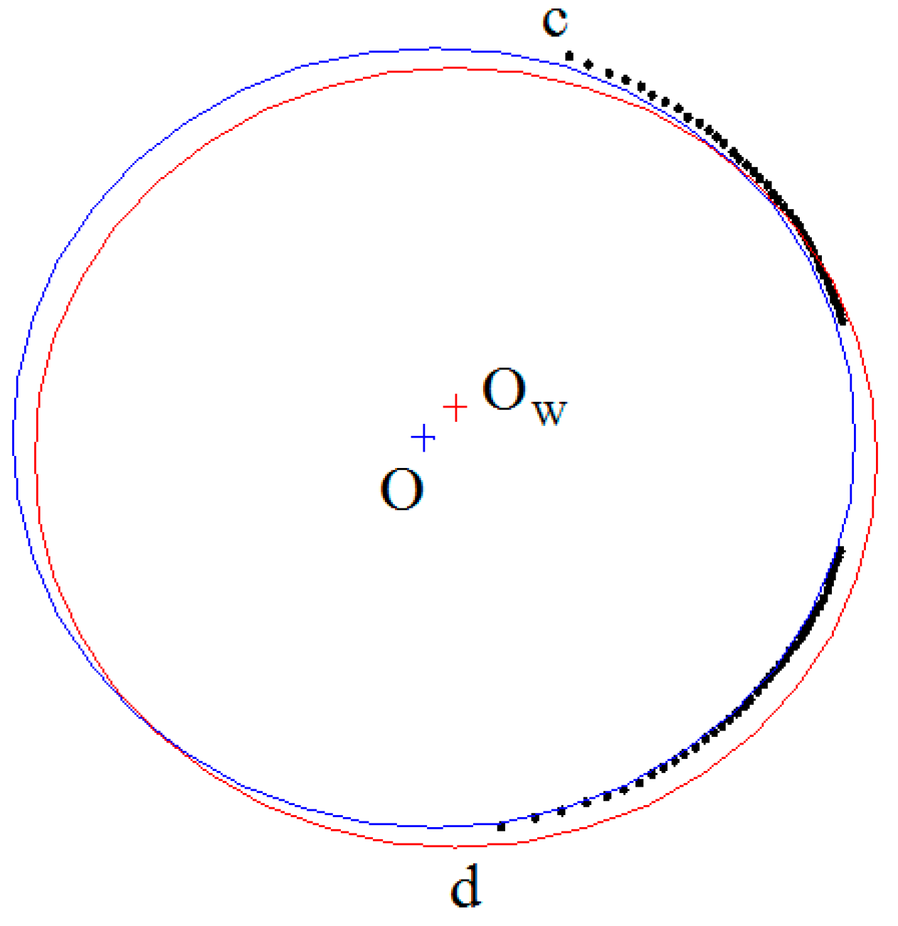
Since arc
cd is at a side of the shaft and the coordinates of points
Qi on
cd have errors, the accuracy of the shaft diameter which is directly measured by fitting points on
cd is poor, as shown in
Figure 8. In
Figure 8, the red circle is a cross-section formed by the virtual plane п
2 intersecting with the shaft and O
w is the center of the red circle. The circle obtained by fitting the black points on
cd is blue with its center at O. To improve the measuring accuracy, the center is determined by fitting black points under the geometrical constraints of arc
cd, and the geometrical constraints for a circle center are shown in
Figure 9.
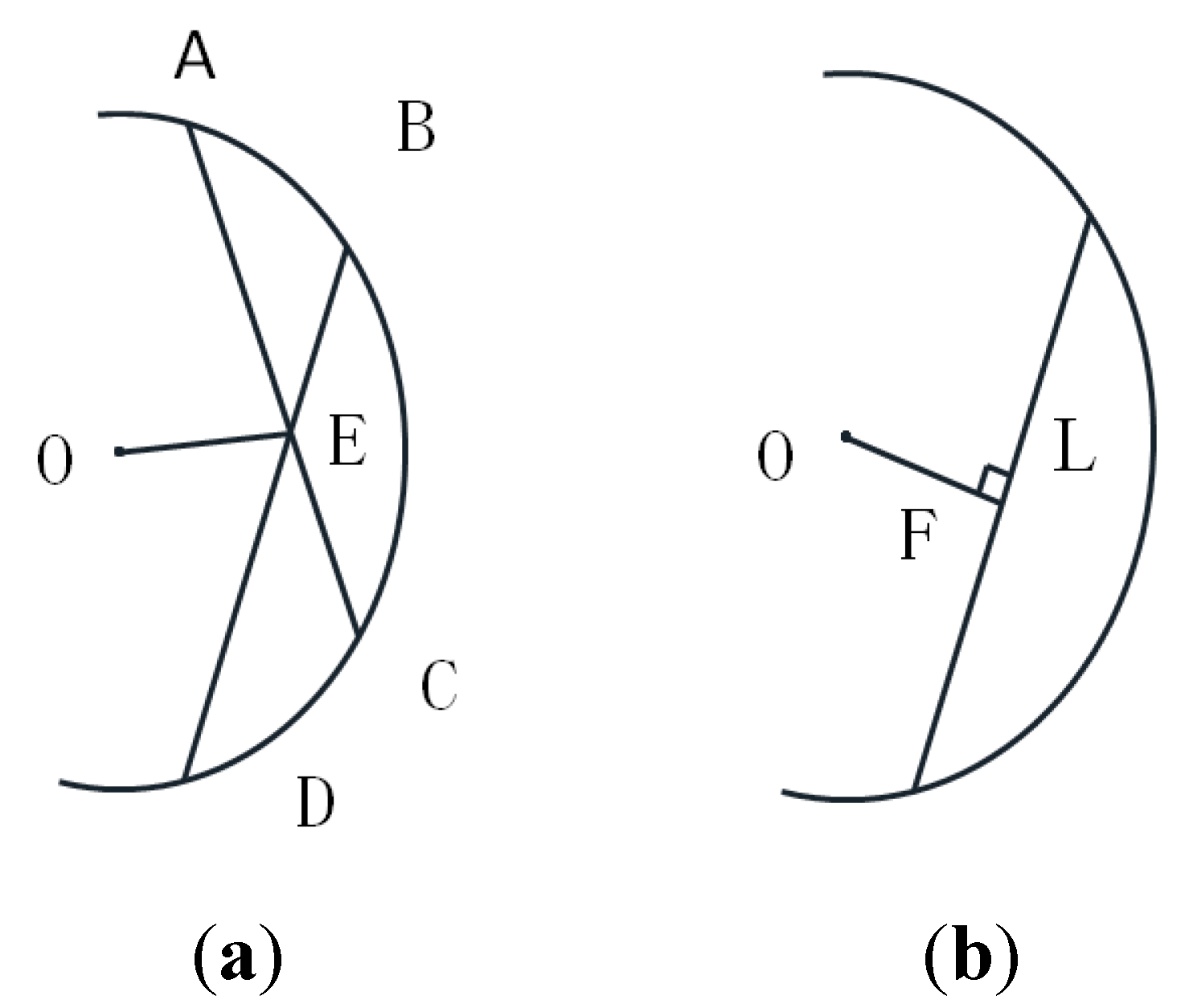
In
Figure 9a, A, B, C, D are the fitting points in the circle and O is the center. Point E is the intersection point of
AC and
BD. From the geometrical feature of a circle, the following relation holds:
where r is radius of the shaft. Setting the center coordinate as (x
0,y
0), the coordinates of the points A, B, C, D are (x
a,y
a), (x
b,y
b), (x
c,y
c), (x
d,y
d). The coordinate (x
e,y
e) of point E can be obtained from points A, B, C, D. Thus, the first objective function can be presented as:
where the value of r is estimated when optimizing Equation (20); n is number of the points.
Figure 8.
Fitting circle by limited data.
Figure 8.
Fitting circle by limited data.
Figure 9.
Geometrical features of a circle. (a) constraint condition1; (b) constraint condition2.
Figure 9.
Geometrical features of a circle. (a) constraint condition1; (b) constraint condition2.
As shown in
Figure 9b, F is the midpoint of the chord L. Thus, line OF is perpendicular to the chord L and can be presented as:
Therefore, the center coordinate can be determined by Equations (20) and (21):
Minimizing Equation (22) is a nonlinear minimization problem, which can be solved by the Levenberg-Marquardt algorithm. The initial value of the center is obtained by fitting the circle with the points in cd.
Finally, the shaft diameter is obtained by the distance between the points in
cd and the optimized center:
where
d is the diameter of shaft, (x
i,y
i) are coordinates of the points in
cd, (X
0,Y
0) is the coordinate of the optimized center, and n is the number of fitting points.
4. Experiments and Analysis
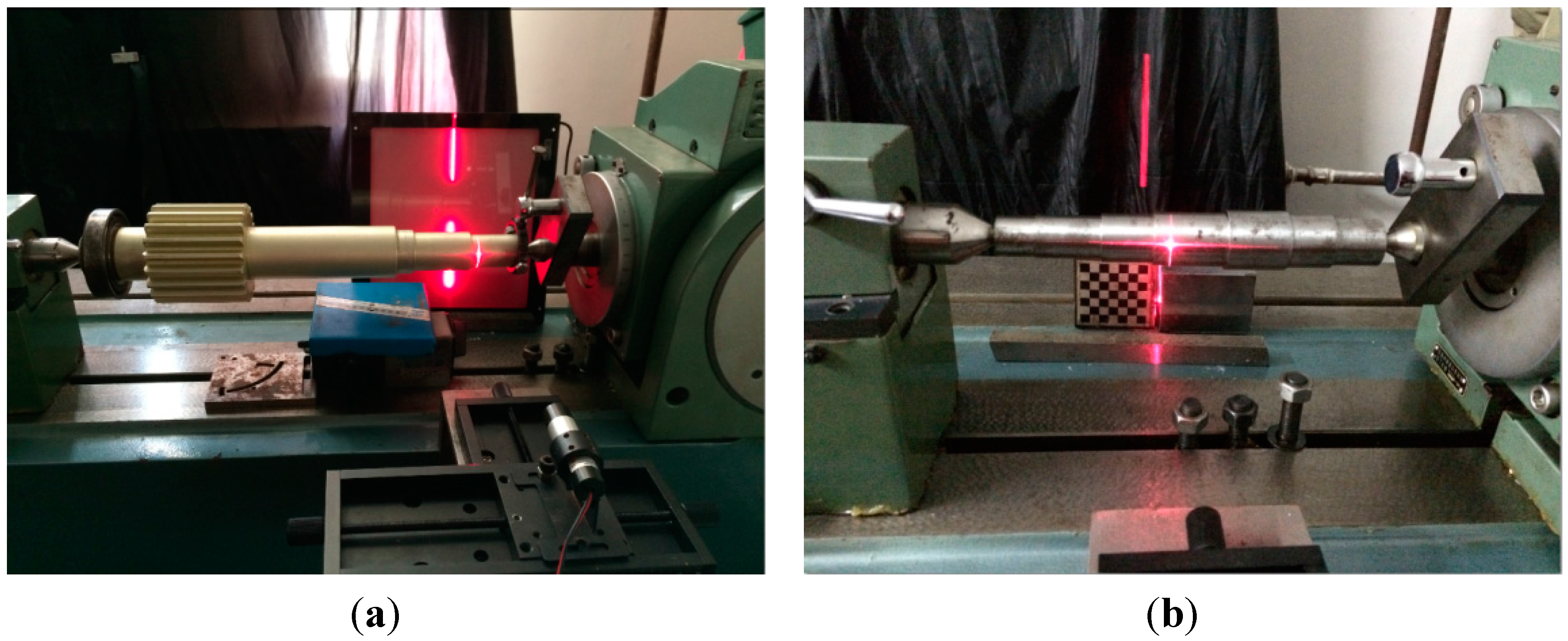
Experiments were conducted to assess the utility of the proposed method. The experimental equipment employed is shown in
Figure 10 and the main parameters of the equipment are shown in
Table 2. The interior parameters of the camera were calibrated by the method presented in
Section 2. Two shafts were used in the experiments; shaft 1 was a four-segment shaft and the shaft surface’s reflection was reduced using a special process, as shown in
Figure 10a. Shaft 2 was a seven-segment shaft, as shown in
Figure 10b. The shafts’ diameters were measured using a micrometer with a resolution of 1 μm.
Figure 10.
Experimental equipment for measuring shafts: (a) shaft 1; (b) shaft 2.
Figure 10.
Experimental equipment for measuring shafts: (a) shaft 1; (b) shaft 2.
Table 2.
Experimental equipment parameters.
Table 2.
Experimental equipment parameters.
| Equipment | Mold NO. | Main Parameters |
|---|
| CCD camera | JAI CCD camera | Resolution: 1376 × 1024 |
| Lens | M0814-MP | Focal length: 25 mm |
| Line projector | LH650-80-3 | Wavelength: 650 nm |
| Mold plane CBC75mm-2.0 | Precision of the grid: 1 μm |
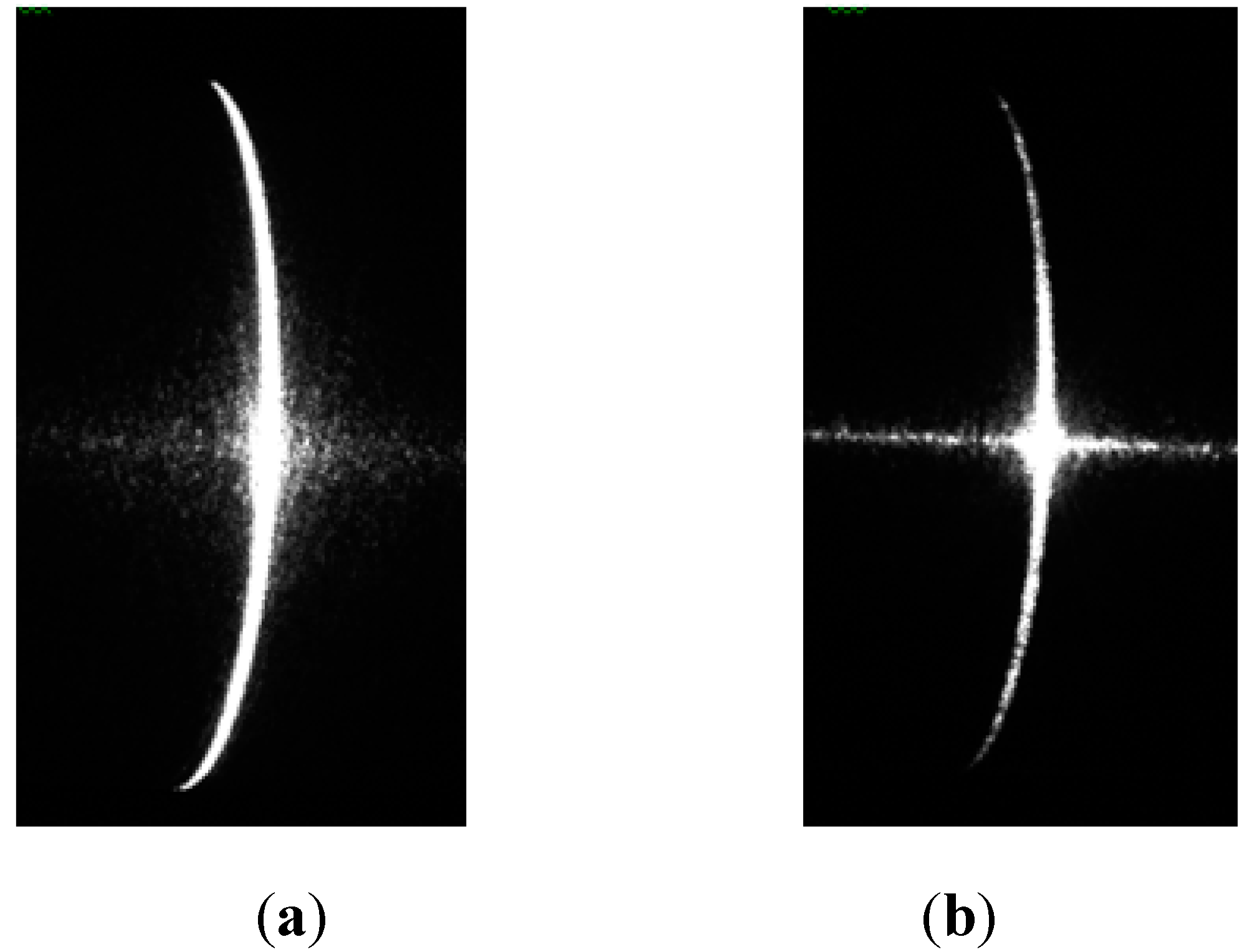
First, the images of the shafts were captured using the camera, as shown in
Figure 11. The diameters of the shafts were measured using the method described in
Section 3. The measurement data are listed in
Table 3 and
Table 4, and the measurement error was less than 25 μm.
Figure 11.
Images of stripes by camera: (a) shaft 1; (b) shaft 2.
Figure 11.
Images of stripes by camera: (a) shaft 1; (b) shaft 2.
Table 3.
Measurement results for shaft 1 (mm).
Table 3.
Measurement results for shaft 1 (mm).
| NO. | 1 | 2 | 3 | 4 |
|---|
| Measurement results | 47.05 | 39.749 | 34.915 | 29.796 |
| Known values | 47.062 | 39.76 | 34.924 | 29.8 |
| Errors | 0.012 | 0.011 | 0.009 | 0.004 |
Table 4.
Measurement results for shaft 2 (mm).
Table 4.
Measurement results for shaft 2 (mm).
| NO. | 1 | 2 | 3 | 4 | 5 | 6 | 7 |
|---|
| Measurement results | 24.761 | 27.661 | 31.456 | 27.474 | 24.596 | 21.696 | 20.091 |
| Known values | 24.753 | 27.664 | 31.473 | 27.492 | 24.621 | 21.687 | 20.113 |
| Errors | 0.008 | 0.003 | 0.017 | 0.018 | 0.025 | 0.009 | 0.022 |
To compare the proposed method with the other methods, the diameters of the shafts were obtained by directly fitting the ellipse and circle. The data for these methods are shown in
Table 5 and
Table 6. The measuring accuracy of the present method was found to be better than that of the other two methods.
Table 5.
Comparison of the measured diameters in shaft1 (mm).
Table 5.
Comparison of the measured diameters in shaft1 (mm).
| NO. | D | Fitting Ellipse | Fitting Circle | Present Method |
|---|
| D1 | Errors | D2 | Errors | D3 | Errors |
|---|
| 1 | 47.062 | 46.992 | 0.07 | 47.034 | 0.028 | 47.05 | 0.012 |
| 2 | 39.76 | 39.659 | 0.101 | 39.698 | 0.062 | 39.749 | 0.011 |
| 3 | 34.924 | 34.773 | 0.151 | 34.827 | 0.097 | 34.915 | 0.009 |
| 4 | 29.8 | 29.741 | 0.059 | 29.73 | 0.07 | 29.796 | 0.004 |
| Mean error | | | 0.095 | | 0.064 | | 0.009 |
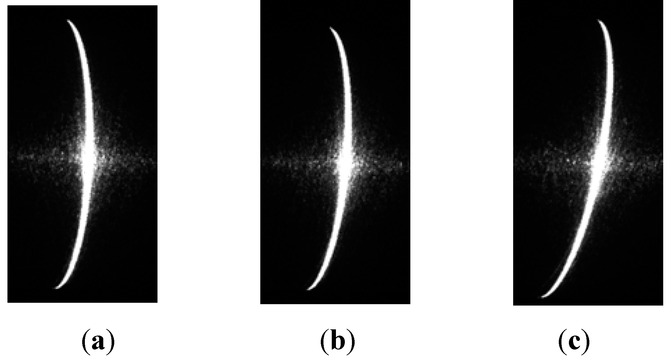
To test the influence of the angle between the light plane and cross-section of the shaft on the proposed method, the shaft diameters were measured by light planes with three different light angles, as shown in
Figure 12. Measurement results are listed in
Table 7 and
Table 8.
Table 6.
Comparison of the measured diameters in shaft 2 (mm).
Table 6.
Comparison of the measured diameters in shaft 2 (mm).
| NO. | D | Fitting Ellipse | Fitting Circle | Present Method |
|---|
| D1 | Errors | D2 | Errors | D3 | Errors |
|---|
| 1 | 24.753 | 24.203 | 0.55 | 24.62 | 0.133 | 24.761 | 0.008 |
| 2 | 27.664 | 27.193 | 0.471 | 27.632 | 0.032 | 27.661 | 0.003 |
| 3 | 31.473 | 30.877 | 0.596 | 31.395 | 0.078 | 31.456 | 0.017 |
| 4 | 27.492 | 27.098 | 0.394 | 27.415 | 0.077 | 27.474 | 0.018 |
| 5 | 24.621 | 24.097 | 0.524 | 24.512 | 0.109 | 24.596 | 0.025 |
| 6 | 21.687 | 21.224 | 0.463 | 21.624 | 0.063 | 21.696 | 0.009 |
| 7 | 20.113 | 19.705 | 0.408 | 19.935 | 0.178 | 20.091 | 0.022 |
| Mean error | | | 0.487 | | 0.096 | | 0.015 |
Figure 12.
Images of stripes at three different angles.
Figure 12.
Images of stripes at three different angles.
From
Table 7 and
Table 8, the light angle appears to have very little effect on the measuring accuracy of the proposed method.
Table 7.
Errors for different angles in shaft 1 (mm).
Table 7.
Errors for different angles in shaft 1 (mm).
| NO. | 1 | 2 | 3 | 4 | Mean Error |
|---|
| a/Errors | 0.012 | 0.011 | 0.009 | 0.004 | 0.009 |
| b/Errors | 0.014 | 0.012 | 0.012 | 0.012 | 0.013 |
| c/Errors | 0.01 | 0.016 | 0.013 | 0.008 | 0.012 |
Table 8.
Errors for different angles in shaft 2 (mm).
Table 8.
Errors for different angles in shaft 2 (mm).
| NO. | 1 | 2 | 3 | 4 | 5 | 6 | 7 | Mean Error |
|---|
| a/Errors | 0.008 | 0.003 | 0.017 | 0.018 | 0.025 | 0.009 | 0.022 | 0.015 |
| b/Errors | 0.005 | 0.007 | 0.004 | 0.016 | 0.026 | 0.013 | 0.018 | 0.013 |
| c/Errors | 0.008 | 0.013 | 0.025 | 0.017 | 0.028 | 0.009 | 0.022 | 0.017 |
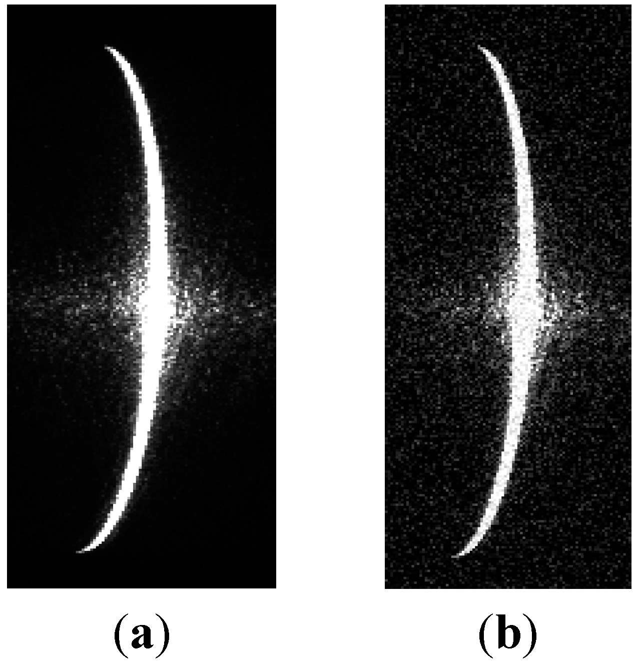
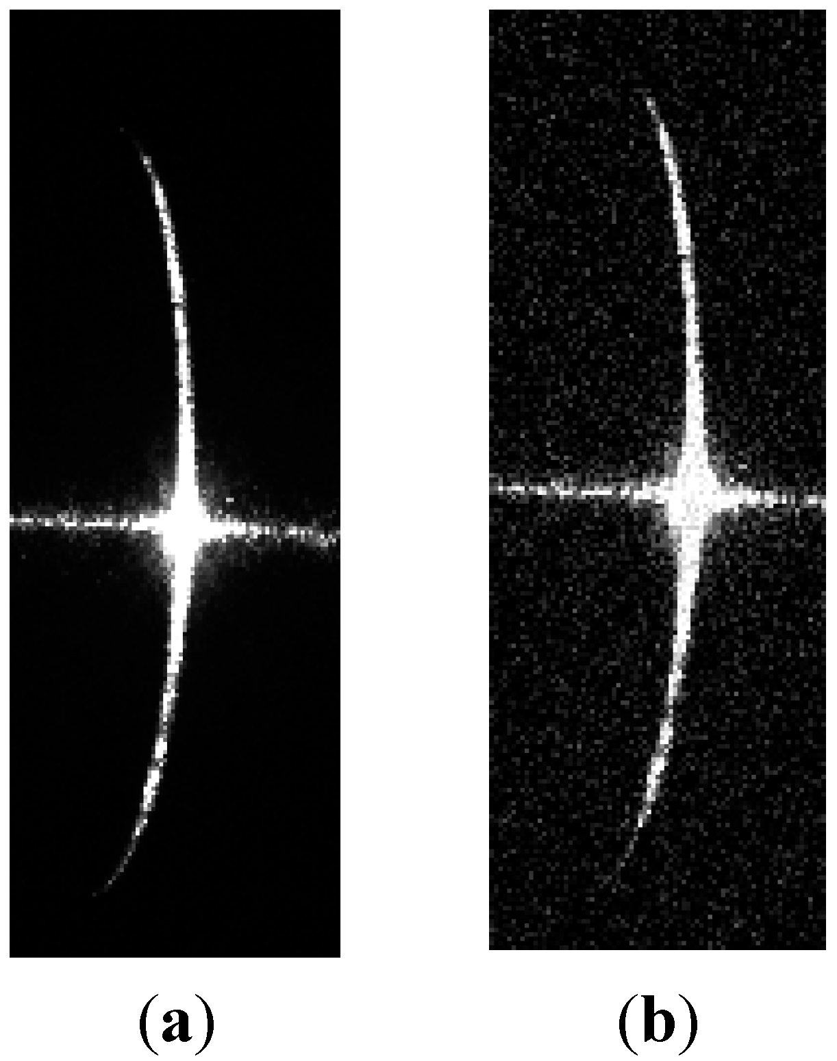
In order to test the influence of noise on the proposed method, noise with a variance of 0.01 and a mean of zero was added to the stripe images of shaft 1 and shaft 2, as shown in
Figure 13 and
Figure 14. The center coordinates of the stripe images with the added noise were extracted by Steger’s algorithm [
14]. The shaft diameters can be determined respectively by the ellipse, circle, and the proposed method fitting the center coordinates. The results are listed in
Table 9 and
Figure 10.
Figure 13.
Images of stripe on shaft 1. (a) normal; (b) added noise.
Figure 13.
Images of stripe on shaft 1. (a) normal; (b) added noise.
Figure 14.
Images of stripe on shaft 2. (a) normal; (b) added noise.
Figure 14.
Images of stripe on shaft 2. (a) normal; (b) added noise.
Table 9.
Measurement results for shaft 1 (mm).
Table 9.
Measurement results for shaft 1 (mm).
| | D | Fitting Ellipse | Fitting Circle | Present Method |
|---|
| D1 | Errors | D2 | Errors | D3 | Errors |
|---|
| Normal | 34.924 | 34.924 | 0.151 | 34.827 | 0.097 | 34.915 | 0.012 |
| Added noise | 34.924 | 34.896 | 0.028 | 34.837 | 0.087 | 34.918 | 0.006 |
| | 0.123 | | 0.01 | | 0.003 | |
Table 10.
Measurement results for shaft 2 (mm).
Table 10.
Measurement results for shaft 2 (mm).
| | D | Fitting Ellipse | Fitting Circle | Present Method |
|---|
| D1 | Errors | D2 | Errors | D3 | Errors |
|---|
| Normal | 31.473 | 30.877 | 0.596 | 31.395 | 0.078 | 31.456 | 0.017 |
| Added noise | 31.473 | 30.762 | 0.711 | 31.421 | 0.052 | 31.47 | 0.003 |
| | 0.115 | | 0.026 | | 0.014 | |
Here, the shaft diameters D were obtained by a micrometer, and
is change of the shaft diameter measurements before and after the added noise. As seen in
Table 9 and
Table 10, the noise has little effect on the measuring accuracy of the proposed method.


