
Reliable Fusion of Stereo Matching and Depth Sensor for High Quality Dense Depth Maps

Abstract
:1. Introduction

- We incorporated texture information as a constraint. The texture variance and gradient is used to restrict the range of the potential disparities for each pixel. In textureless and repetitive regions (which often cause ambiguities when stereo matching), we restrict the possible disparities for a neighborhood centered on each pixel to a limited range around the values suggested by the Xtion. This reduces the errors and strengthens the compact distribution of the disparities in a segment.
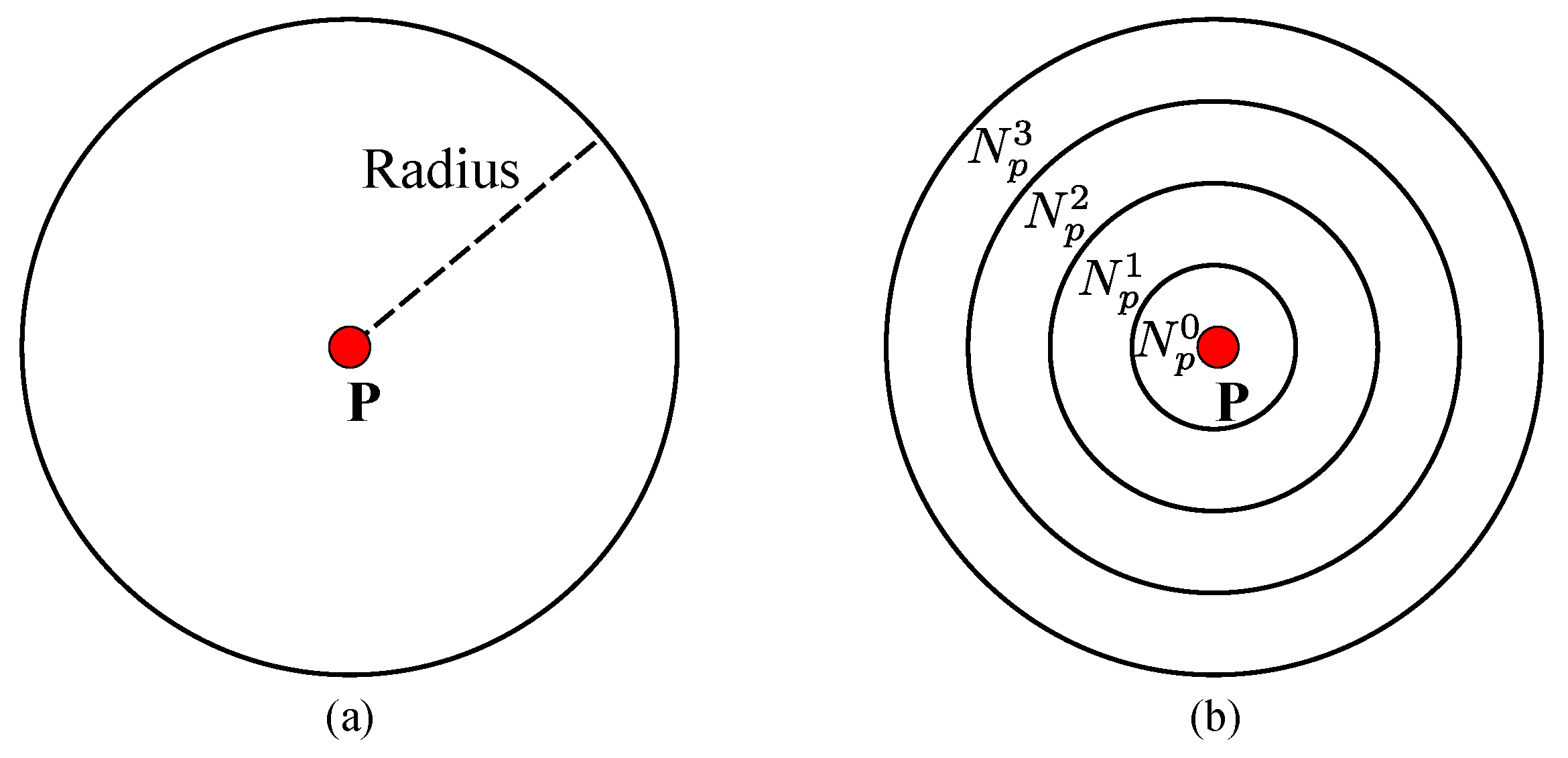
- We propose the multiscale pseudo-two-layer image model (MPTL; Figure 2) to represent the relationships between disparities at different pixels and segments. We consider the disparities from the Xtion as the prior knowledge and use it to increase the robustness to luminance variance and to strengthen the 3D planar surface bias. Furthermore, considering the spatial structures of segments obtained from the depth sensor, we treat the segmentation as a soft constraint to reduce matching ambiguities caused by under- and over-segmentation. Here, pixels with similar colors, but on different objects are grouped into one segment, and pixels with different colors, but on the same object are partitioned into different segments. Additionally, we only retain the disparity discontinuities that align with object boundaries from geometrically-smooth, but strong color gradient regions.

2. Previous Work
3. Method
3.1. Pre-Processing

- -
- and have the same matching point in under their current disparity value;
- -
- ;
- -
- and belong to different segments.


| D: | Disparity map | : | Disparity value of pixel p | Π: | Seed image |
| : | Initial disparity map of rectified left image | : | Initial disparity map of rectified right image | : | Rectified left DSLR image |
| : | Rectified right DSLR image | R: | Reliable segment | : | Unreliable segment |
| S: | Stable segment | : | Unstable segment | : | i-th segment |
| : | i-th stable segment | : | Fitted plane of stable segment | : | Segment that contains pixel p |
| : | i-th segment | : | Minimum disparity | : | maximum disparity |
| ϖ: | Segment boundary pixels | : | Pixel’s potential minimum disparity | : | Pixel’s potential maximum disparity |
| : | Minimum fitted disparity of the i-th stable segment | : | Minimum fitted disparity of the i-th stable segment |
3.2. Problem Formulation
- -
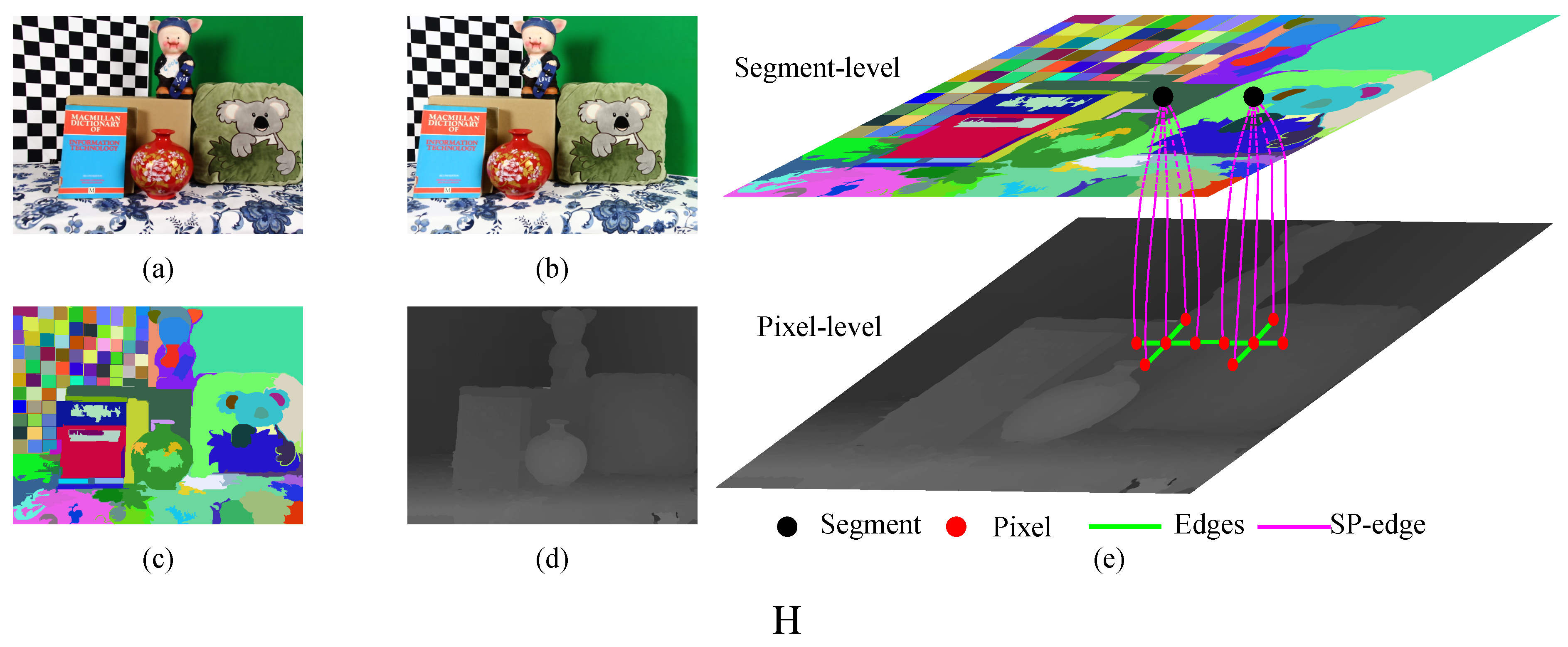
- The pixel-level component, which improves the robustness against the luminance variance (Section 3.3) and strengthens the smoothness of disparities between neighboring pixels and segments (Section 3.4). Nodes at this level represent reliable pixels from stable and unstable segments. The edges between reliable pixels represent different types of smoothness terms.
- -
- The edge that connects two level components (the SP-edge), which uses the texture variance and gradient as a guide to restrict the scope of potential disparities (Section 3.5).
- -
- The segment-level component, which incorporates the information from the Xtion as prior knowledge to capture the spatial structure of each stable segment and to maintain the relationship between neighboring stable segments (Section 3.6). Each node at this level represents a stable segment.
3.3. Improved Luminance Consistency Term
3.4. Hybrid Smoothness Term
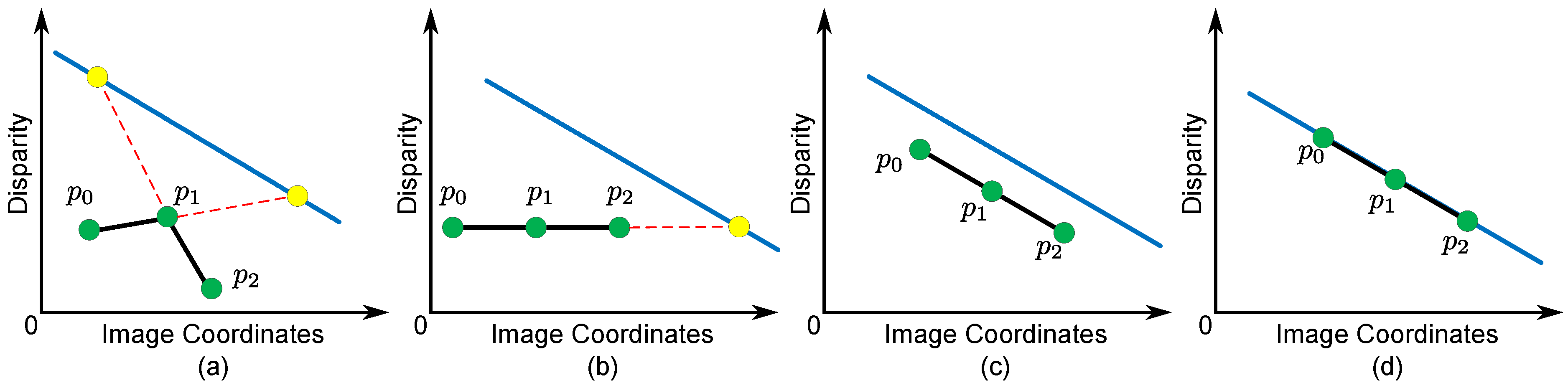
- -
- Case I: When , the disparity gradients of pixels in are not constant (). This case violates the basic segmentation assumptions that the disparity variance of neighboring pixels is smooth, so a large penalty is added to prevent it from happening in our model (see Figure 5a).
- -
- Cases II, III and IV: When , the disparity gradients of pixels in are constant (). This means that the variance of the disparities is smooth. Furthermore, our model checks the relationship between all pixels in and (see Figure 5b–d). does not penalize the disparity assignment if all pixels in belong to (Case IV in Figure 5d), because it is reasonable to assume that the local structure of is the same as the spatial structure of . Note that we impose a larger penalty to Case II than to Case III to strengthen the similarity between the spatial structure of and .

3.5. Texture Term

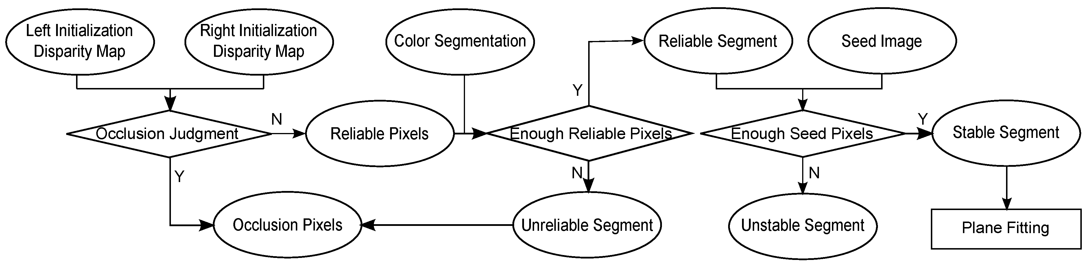
- -
- When is a stable segment () and contains sufficient seed pixels (), is equal to . In this case, there are enough seed pixels from the Xtion to denote a guide for the variance of disparities of p. If p is in the textureless or repetitive region, is small. This indicates that stereo matching may fail in these regions, and a small search range should be used around disparities from the Xtion. In contrast, if p is in the rich textured region or object boundaries, is large. This indicates that disparities from the Xtion may be susceptible to noise and problems caused by rich texture regions where disparities obtained from stereo matching are more reliable. Then, a broader search range should be used, so that we can extract better results not observed by the Xtion.
- -
- When is a stable segment (), but there are not enough seed pixels around p (), is equal to . In this case, although there are some seed pixels from the Xtion, they are not enough to represent the disparity variance around p. On the other hand, because each stable segment is viewed as a 3D fitted plane, the search range for the potential disparities is limited by the fitted disparity of and the disparity variance buffer ().
- -
- When is an unstable segment (), is the minimum disparity ().
3.6. 3D Plane Bias Term
3.7. Optimization
- -
- Proposal A: Uniform value-based proposal. All disparities in the proposal are assigned to a discrete disparity, in the range of to .
- -
- Proposal B: The hierarchical belief propagation-based algorithm [41] is applied to generate proposals with different segmentation maps.
- -
- Proposal C: The joint disparity map and color consistency estimation method [42], which combines mutual information, a SIFT descriptor and segment-based plane-fitting techniques.
3.8. Post-Processing
4. Results and Discussion
| 0.1 | 50 | 3 | 5 | 35 | 1.5 | 200 | 12 | 200 | 40 | 40 | 15 | 15 | 10 |
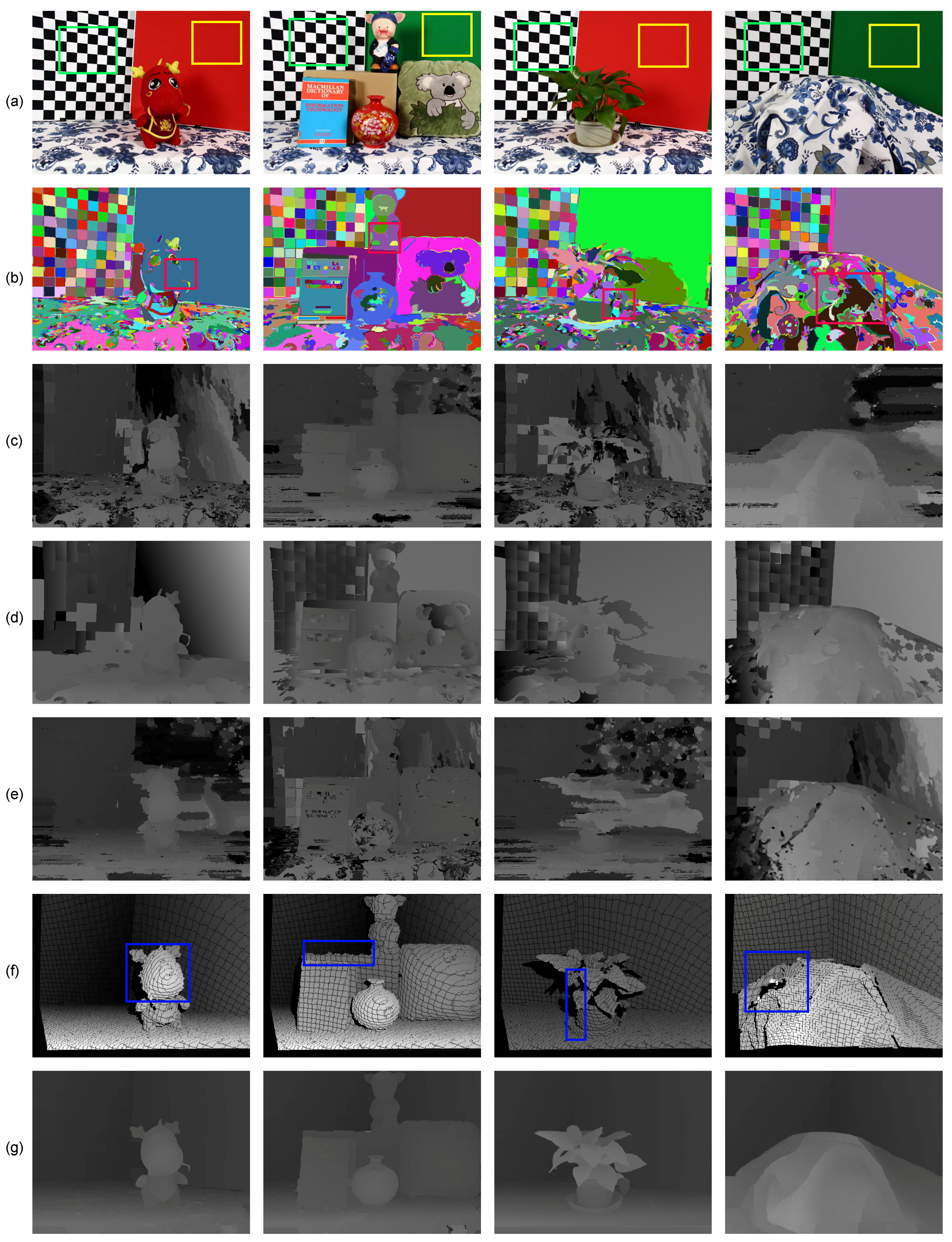
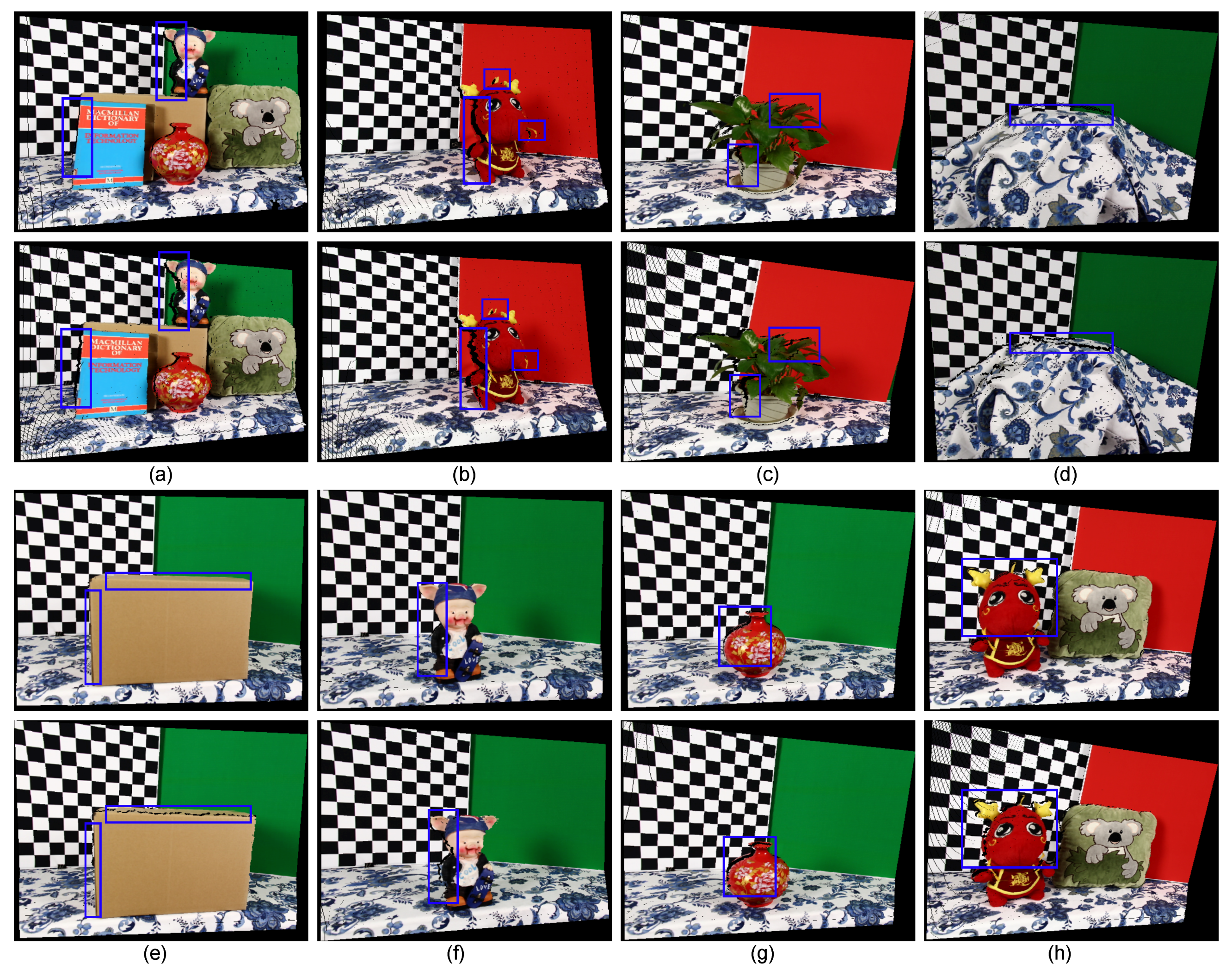
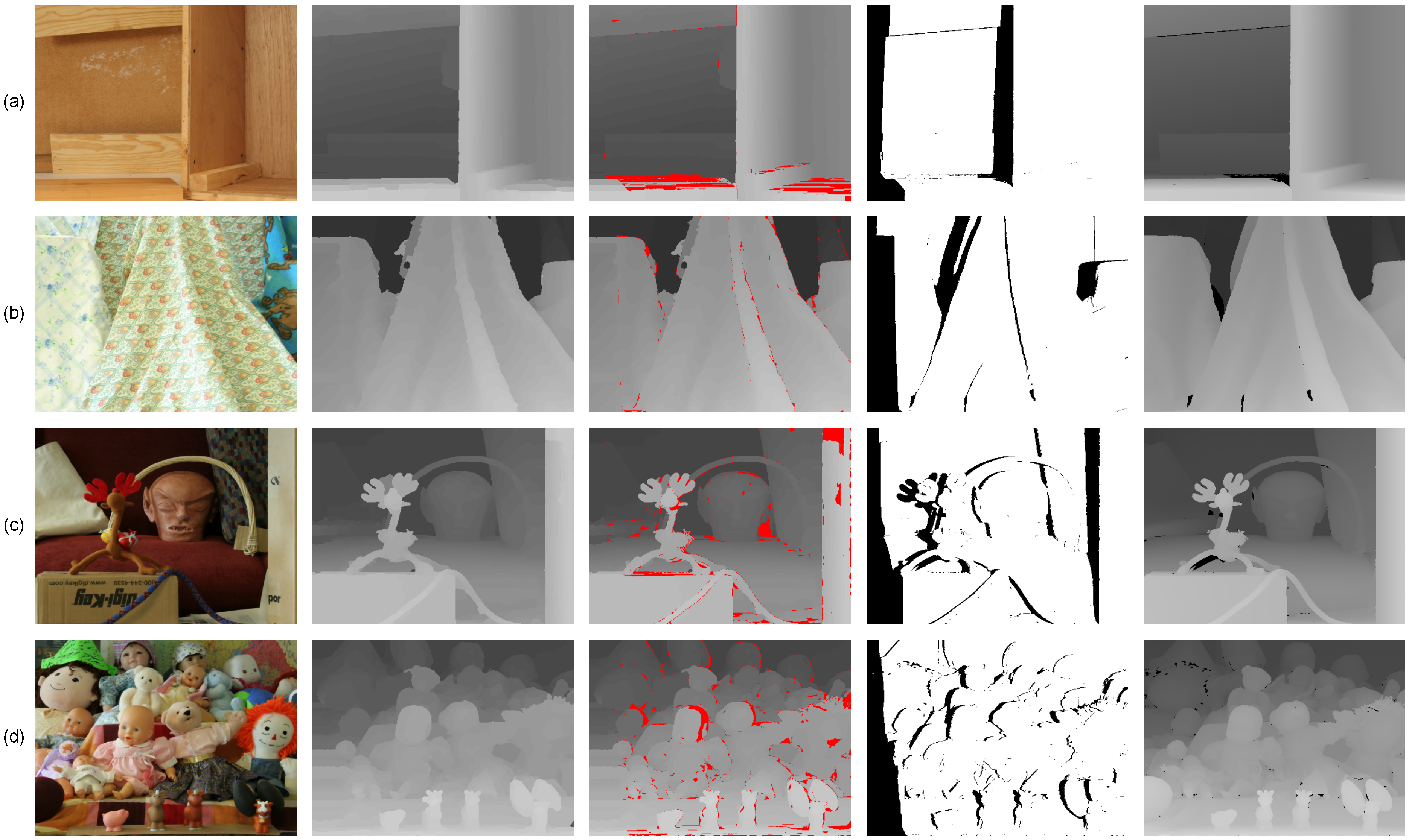
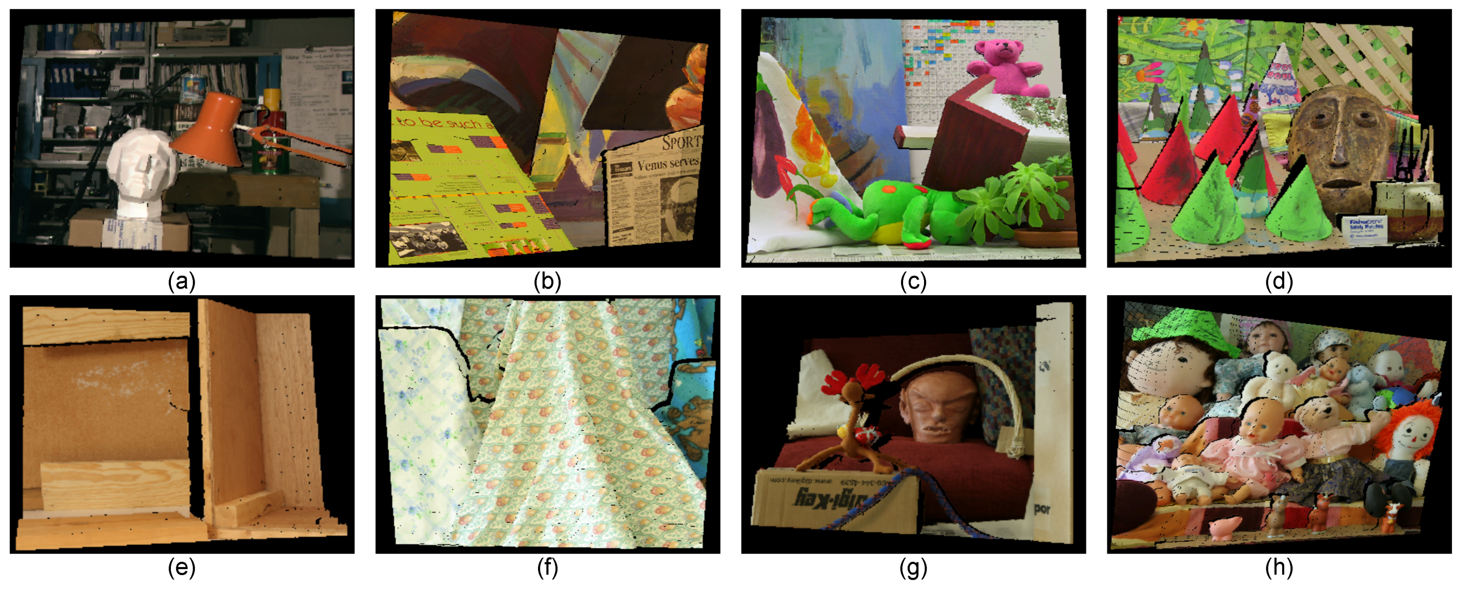
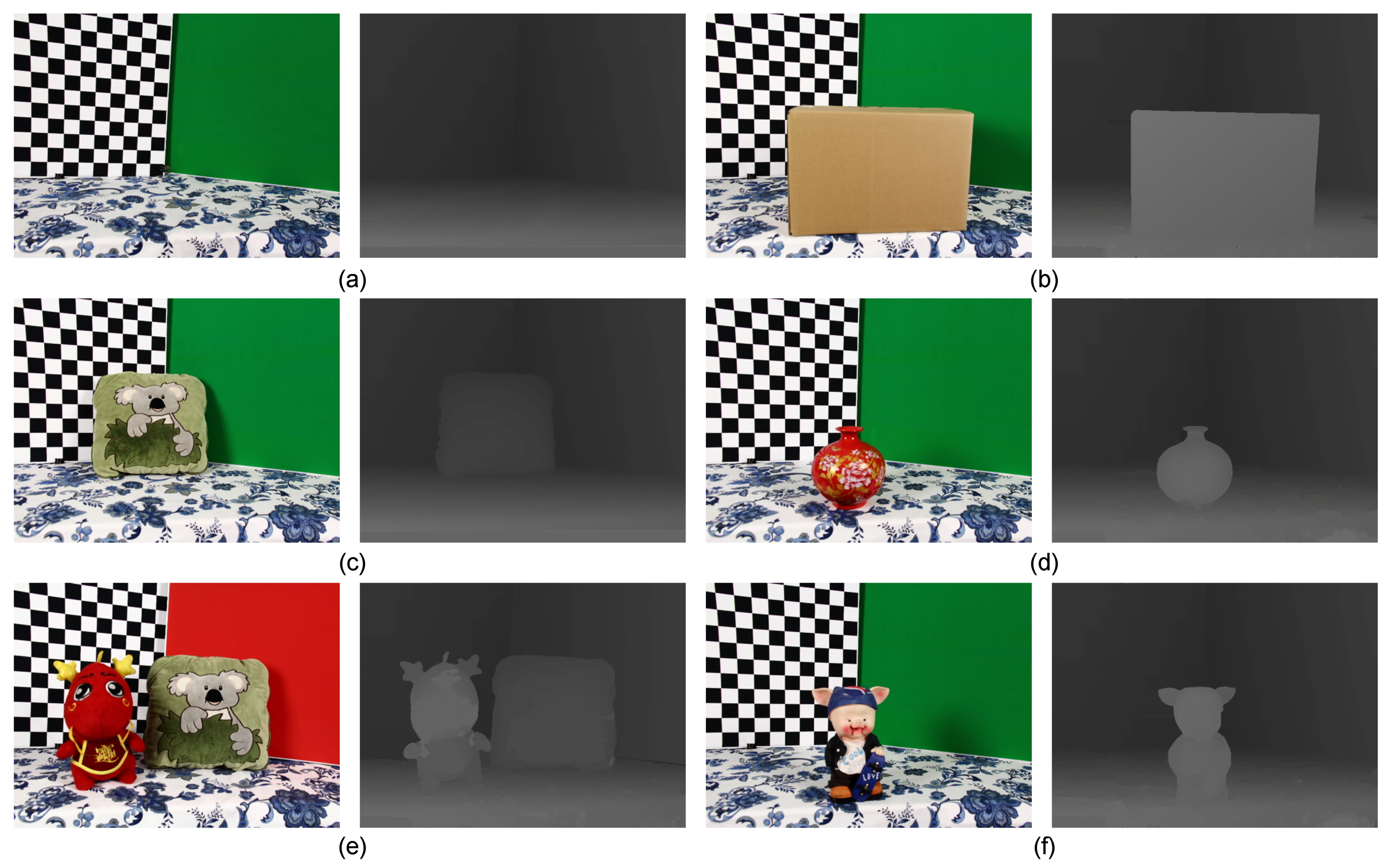
4.1. Qualitative Evaluation Using the Real-World Datasets


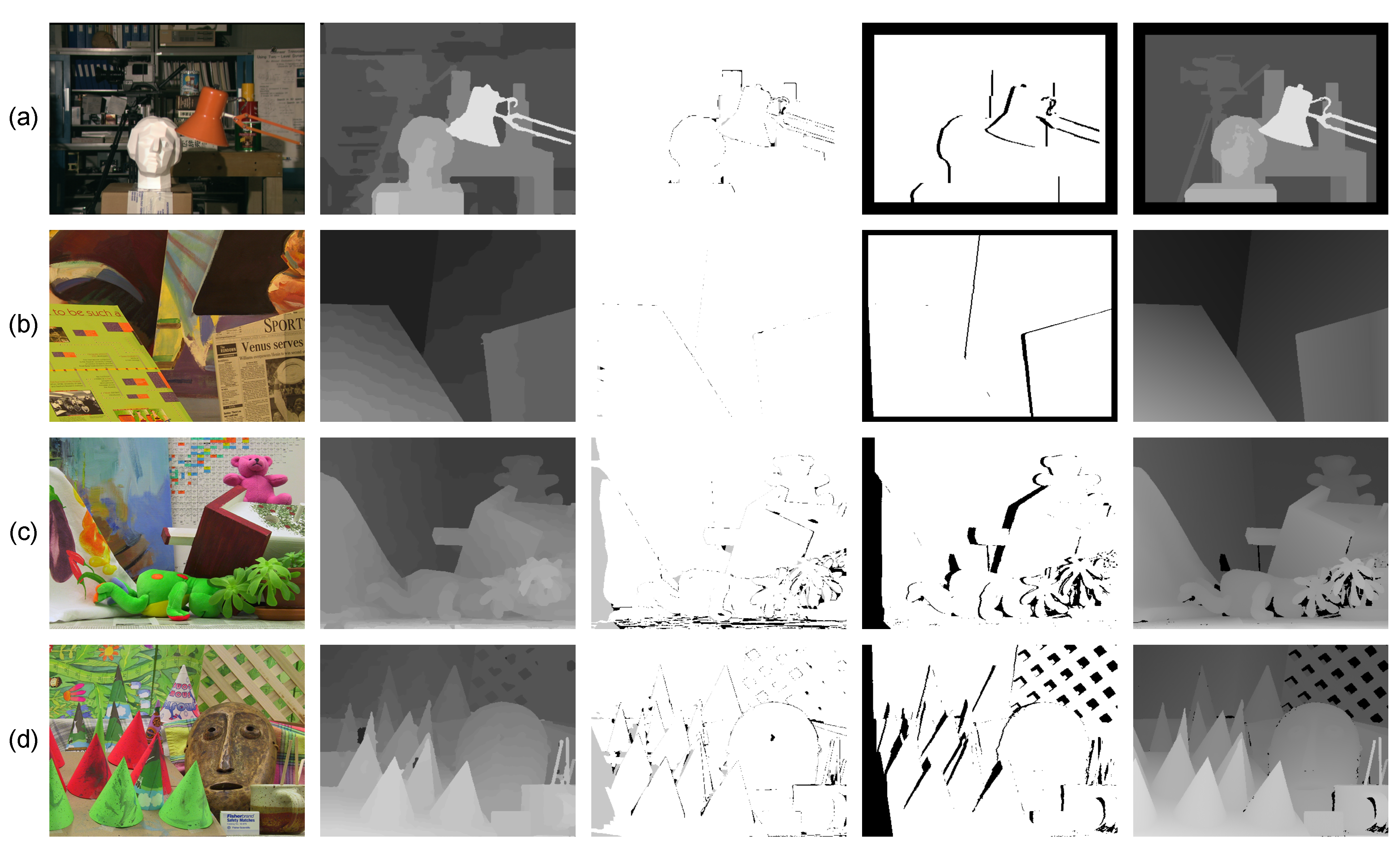
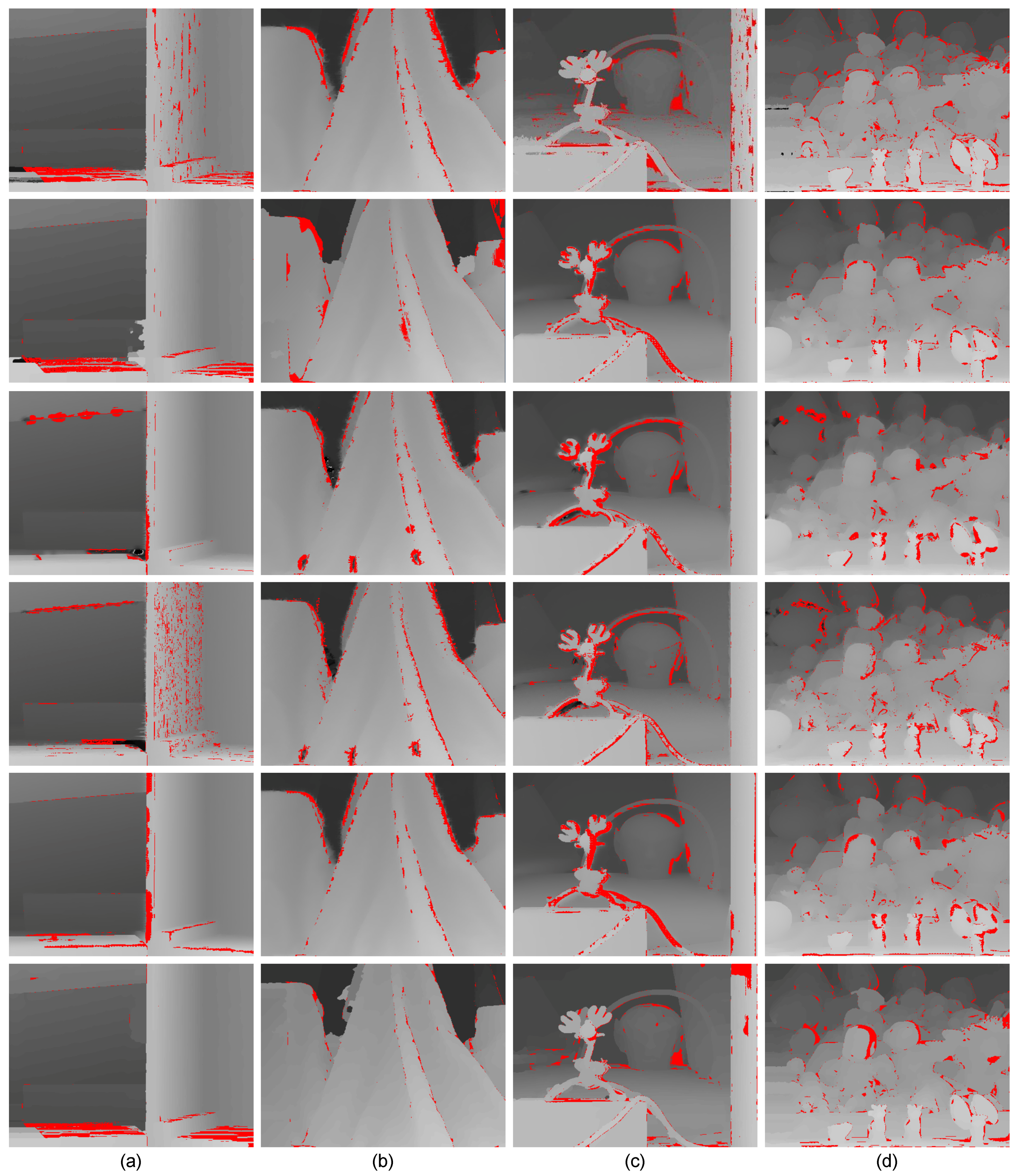
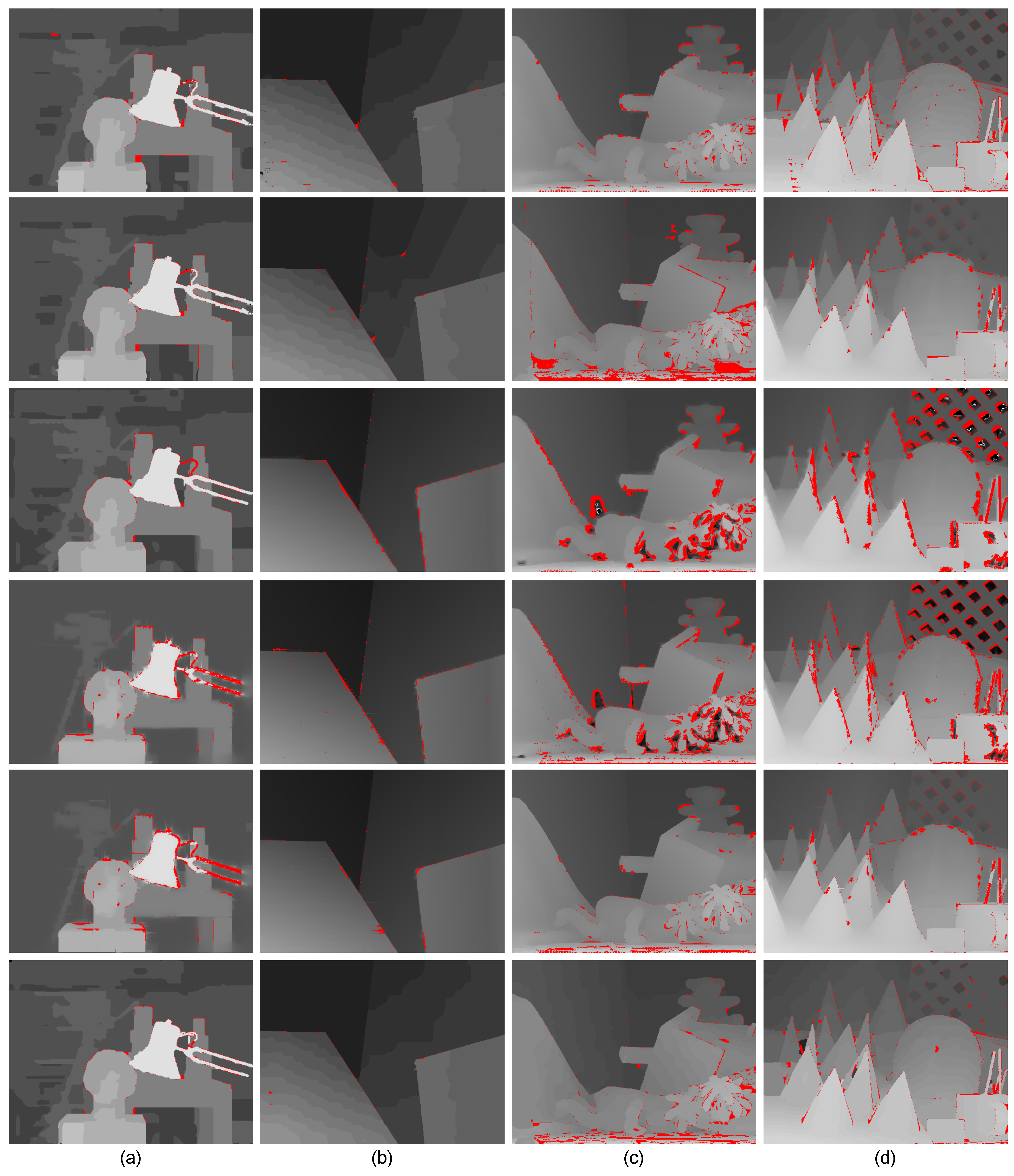
4.2. Quantitative Evaluation Using the Middlebury Datasets


- -
- Noise and outliers are significantly reduced, mainly because of the improved luminance consistency term and the texture term.
- -
- The method obtains precise disparities for slanted or highly-curved surfaces of objects with complex geometric characteristics, mainly because of the 3D plane bias term.
- -
- Ambiguous matchings caused by over-segmentation or under-segmentation are overcome and disparity variances become smoother, mainly because of the hybrid smoothness term.


| The Percentages of Error Pixels (%) | ||||||||||
|---|---|---|---|---|---|---|---|---|---|---|
| Tsukuba | Venus | Teddy | Conse | Wood1 | Colth4 | Reimdeor | Dools | Averages | ||
| Zhu et al. [20] | 1.16 | 0.14 | 2.83 | 3.47 | 5.38 | 3.74 | 5.83 | 5.46 | 3.50 | |
| Wang et al. [23] | 0.89 | 0.12 | 6.39 | 2.14 | 4.05 | 3.81 | 3.55 | 2.71 | 2.96 | |
| Yang et al. [52] | 0.94 | 0.26 | 5.65 | 7.18 | 1.76 | 2.60 | 4.43 | 4.13 | 3.37 | |
| Jaesik et al. [53,55] | 2.38 | 0.56 | 5.59 | 6.28 | 3.72 | 2.88 | 4.04 | 4.69 | 3.77 | |
| James et al. [54] | 2.90 | 0.29 | 2.12 | 2.83 | 2.74 | 2.32 | 5.02 | 4.02 | 2.78 | |
| Ours | 0.79 | 0.10 | 3.49 | 2.06 | 4.35 | 1.03 | 4.31 | 4.78 | 2.61 | |

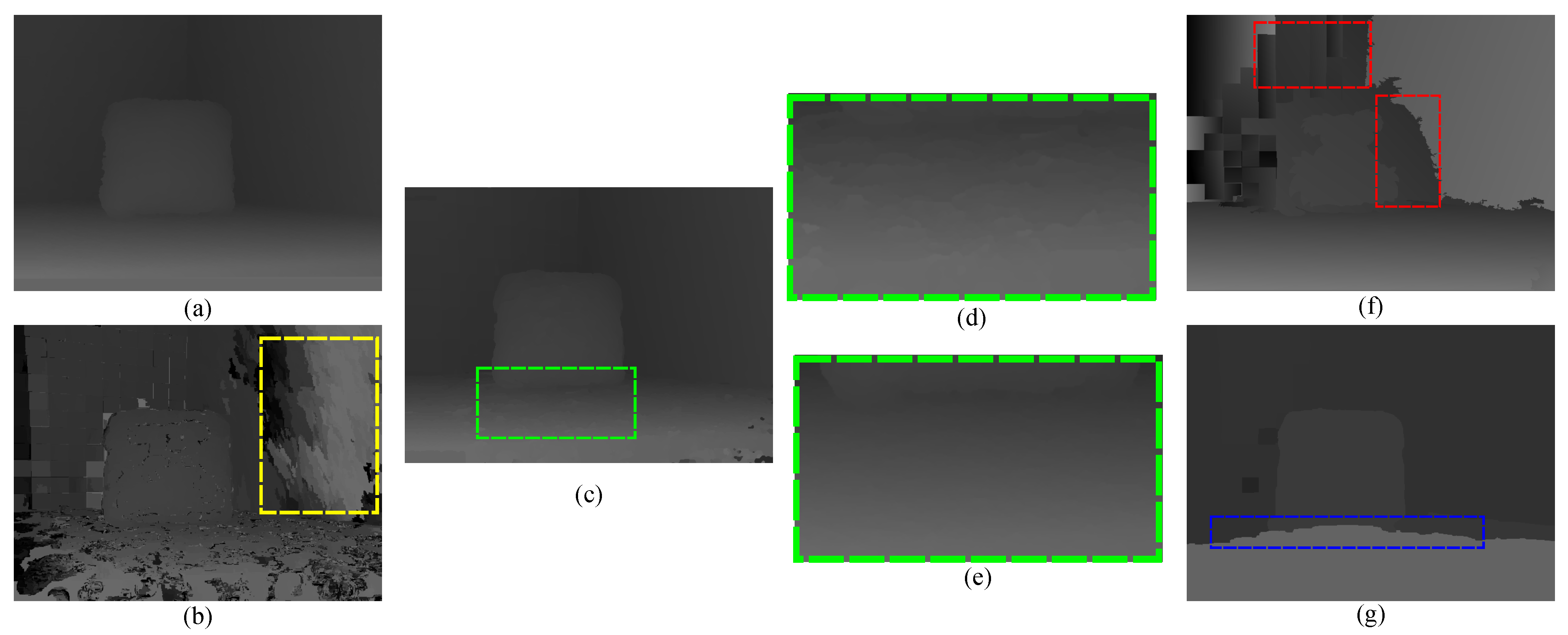
4.3. Evaluation Results for Each Term

| Tsukuba | Venus | Teddy | Cones | Averages | |||||||||||||||
|---|---|---|---|---|---|---|---|---|---|---|---|---|---|---|---|---|---|---|---|
| nonocc | all | disc | nonocc | all | disc | nonocc | all | disc | nonocc | all | disc | nonocc | all | disc | |||||
| Texture term off | 2.04 | 2.12 | 5.78 | 0.81 | 1.03 | 3.09 | 5.43 | 10.2 | 13.25 | 2.79 | 8.26 | 6.35 | 2.77 | 5.40 | 7.12 | ||||
| Luminance term off | 1.01 | 1.65 | 4.78 | 0.11 | 0.25 | 1.54 | 5.49 | 11.20 | 14.92 | 2.88 | 8.47 | 7.74 | 2.37 | 5.39 | 7.25 | ||||
| Smoothness term off | 1.39 | 2.14 | 4.94 | 0.85 | 0.93 | 2.02 | 6.57 | 13.01 | 14.80 | 3.28 | 7.50 | 7.13 | 3.02 | 5.90 | 7.22 | ||||
| Plane bias term off | 0.88 | 1.49 | 4.86 | 0.23 | 0.65 | 2.27 | 4.53 | 9.30 | 10.63 | 2.90 | 7.96 | 8.96 | 2.14 | 4.76 | 6.68 | ||||
| All terms on | 0.79 | 1.21 | 4.30 | 0.10 | 0.21 | 1.27 | 3.49 | 9.04 | 10.90 | 2.06 | 7.05 | 5.80 | 1.61 | 4.37 | 5.56 | ||||
4.4. Computational Time Analyses
| Dragon | Book | Plant | Tableclotd | Board | Box | Kola | Vase | Piggy | Dragon and Piggy | |
|---|---|---|---|---|---|---|---|---|---|---|
| Running Time (m): | 22.15 | 20.54 | 22.16 | 24.31 | 21.51 | 24.26 | 23.43 | 22.30 | 19.44 | 23.04 |
| Tsukuba | Venus | Teddy | Cones | Wood1 | Cloth4 | Reindeer | Dolls | |
|---|---|---|---|---|---|---|---|---|
| Running Time (m): | 1.03 | 1.19 | 4.08 | 4.57 | 8.18 | 7.44 | 7.02 | 8.31 |
| Disparity Map Resolution: | ||||||||
| Maximum Disparity: | 15 | 19 | 59 | 59 | 71 | 69 | 67 | 73 |
5. Conclusions
Acknowledgments
Author Contributions
Conflicts of Interest
References
- Díaz-Vilariño, L.; Khoshelham, K.; Martínez-Sánchez, J.; Arias, P. 3D modeling of building indoor spaces and closed doors from imagery and point clouds. Sensors 2015, 15, 3491–3512. [Google Scholar] [CrossRef] [PubMed]
- Pan, S.; Shi, L.; Guo, S. A kinect-based real-time compressive tracking prototype system for amphibious spherical robots. Sensors 2015, 15, 8232–8252. [Google Scholar] [CrossRef] [PubMed]
- Yebes, J.J.; Bergasa, L.M.; García-Garrido, M. Visual object recognition with 3D-aware features in KITTI urban scenes. Sensors 2015, 15, 9228–9250. [Google Scholar] [CrossRef] [PubMed]
- Tanimoto, M.; Tehrani, M.P.; Fujii, T.; Yendo, T. Free-viewpoint TV. IEEE Signal Process. Mag. 2011, 28, 67–76. [Google Scholar] [CrossRef]
- Liu, J.; Li, C.; Mei, F.; Wang, Z. 3D entity-based stereo matching with ground control points and joint second-order smoothness prior. Vis. Comput. 2014, 31, 1–17. [Google Scholar] [CrossRef]
- ASUS Xtion. Available online: www.asus.com/Multimedia/Xtion/ (accessed on 19 August 2015).
- Microsoft Kinect. Available online: www.microsoft.com/zh-cn/kinectforwindows/ (accessed on 19 August 2015).
- Song, X.; Zhong, F.; Wang, Y.; Qin, X. Estimation of kinect depth confidence through self-training. Vis. Comput. 2014, 30, 855–865. [Google Scholar] [CrossRef]
- Scharstein, D.; Szeliski, R. A taxonomy and evaluation of dense two-frame stereo correspondence algorithms. Int. J. Comput. Vis. 2002, 47, 7–42. [Google Scholar] [CrossRef]
- Yoon, K.J.; Kweon, I.S. Adaptive support-weight approach for correspondence search. IEEE Trans. Pattern Anal. Mach. Intell. 2006, 28, 650–656. [Google Scholar] [CrossRef] [PubMed]
- Woodford, O.; Torr, P.; Reid, I.; Fitzgibbon, A. Global stereo reconstruction under second-order smoothness priors. IEEE Trans. Pattern Anal. Mach. Intell. 2009, 31, 2115–2128. [Google Scholar] [CrossRef] [PubMed]
- Bleyer, M.; Rhemann, C.; Rother, C. Patch match stereo-stereo matching with slanted support windows. BMVC 2011, 11, 1–11. [Google Scholar]
- Mei, X.; Sun, X.; Dong, W.; Wang, H.; Zhang, X. Segment-tree based Cost Aggregation for Stereo Matching. In Proceedings of the 2013 IEEE Conference on Computer Vision and Pattern Recognition, Portland, OR, USA, 23–28 June 2013; pp. 313–320.
- Wang, L.; Yang, R. Global Stereo Matching Leveraged by Sparse Ground Control Points. In Proceedings of the IEEE Conference Computer Vision and Pattern Recognition, Providence, RI, USA, 20–25 June 2011; pp. 3033–3040.
- LiDAR. Available online: www.lidarusa.com (accessed on 19 August 2015).
- 3DV Systems. Available online: www.3dvsystems.com (accessed on 19 August 2015).
- Photonix Mixer Device for Distance Measurement. Available online: www.pmdtec.com (accessed on 19 August 2015).
- Khoshelham, K.; Elberink, S.O. Accuracy and resolution of kinect depth data for indoor mapping applications. Sensors 2012, 12, 1437–1454. [Google Scholar] [CrossRef] [PubMed]
- Zhu, J.; Wang, L.; Gao, J.; Yang, R. Spatial-temporal fusion for high accuracy depth maps using dynamic MRFs. IEEE Trans. Pattern Anal. Mach. Intell. 2010, 32, 899–909. [Google Scholar] [PubMed]
- Zhu, J.; Wang, L.; Yang, R.; Davis, J.E.; Pan, Z. Reliability fusion of time-of-flight depth and stereo geometry for high quality depth maps. IEEE Trans. Pattern Anal. Mach. Intell. 2011, 33, 1400–1414. [Google Scholar]
- Yang, Q.; Tan, K.H.; Culbertson, B.; Apostolopoulos, J. Fusion of Active and Passive Sensors for Fast 3D Capture. In Proceedings of the IEEE International Workshop on Multimedia Signal Processing, Saint Malo, France, 4–6 October 2010; pp. 69–74.
- Zhang, S.; Wang, C.; Chan, S. A New High Resolution Depth Map Estimation System Using Stereo Vision and Depth Sensing Device. In Proceedings of the IEEE 9th International Colloquium on Signal Processing and its Applications, Kuala Lumpur, Malaysia, 8–10 March 2013; pp. 49–53.
- Wang, Y.; Jia, Y. A fusion framework of stereo vision and Kinect for high-quality dense depth maps. Comput. Vis. 2013, 7729, 109–120. [Google Scholar]
- Somanath, G.; Cohen, S.; Price, B.; Kambhamettu, C. Stereo Kinect for High Resolution Stereo Correspondences. In Proceedings of the IEEE International Conference on 3DTV-Conference, Seattle, Washington, DC, USA, 29 June–1 July 2013; pp. 9–16.
- Zhang, Z. A flexible new technique for camera calibration. IEEE Trans. Pattern Anal. Mach. Intell. 2000, 22, 1330–1334. [Google Scholar] [CrossRef]
- Herrera, C.; Kannala, J.; Heikkilä, J. Joint depth and color camera calibration with distortion correction. IEEE Trans. Pattern Anal. Mach. Intell. 2012, 34, 2058–2064. [Google Scholar] [CrossRef] [PubMed]
- Yang, Q. A Non-Local Cost Aggregation Method for Stereo Matching. In Proceedings of the IEEE Conference on Computer Vision and Pattern Recognition, Providence, RI, USA, 16–21 June 2012; pp. 1402–1409.
- Christoudias, C.M.; Georgescu, B.; Meer, P. Synergism in low level vision. IEEE Intern. Conf. Pattern Recognit. 2002, 4, 150–155. [Google Scholar]
- Bleyer, M.; Rother, C.; Kohli, P. Surface Stereo with Soft Segmentation. In Proceedings of the IEEE Conference on Computer Vision and Pattern Recognition (CVPR), San Francisco, CA, USA, 13–18 June 2010; pp. 1570–1577.
- Wei, Y.; Quan, L. Asymmetrical occlusion handling using graph cut for multi-view stereo. IEEE Intern. Conf. Pattern Recognit. 2005, 2, 902–909. [Google Scholar]
- Hu, X.; Mordohai, P. A quantitative evaluation of confidence measures for stereo vision. IEEE Trans. Pattern Anal. Mach. Intell. 2012, 34, 2121–2133. [Google Scholar] [PubMed]
- Liu, Z.; Han, Z.; Ye, Q.; Jiao, J. A New Segment-Based Algorithm for Stereo Matching. In Proceedings of the IEEE International Conference on Mechatronics and Automation, Changchun, China, 9–12 August 2009; pp. 999–1003.
- Rao, A.; Srihari, R.K.; Zhang, Z. Spatial color histograms for content-based image retrieval. In Proceedings of the 11th IEEE International Conference on Tools with Artificial Intelligence, Chicago, IL, USA, 9–11 November 1999; pp. 183–186.
- Lempitsky, V.; Rother, C.; Blake, A. Logcut-Efficient Graph Cut Optimization for Markov Random Fields. In Proceedings of the IEEE 11th International Conference on Computer Vision, Rio de Janeiro, Brazil, 14–21 October 2007; pp. 1–8.
- Boykov, Y.; Veksler, O.; Zabih, R. Fast approximate energy minimization via graph cuts. IEEE Trans. Pattern Anal. Mach. Intell. 2001, 23, 1222–1239. [Google Scholar] [CrossRef]
- Kolmogorov, V.; Zabin, R. What energy functions can be minimized via graph cuts? IEEE Trans. Pattern Anal. Mach. Intell. 2004, 26, 147–159. [Google Scholar] [CrossRef] [PubMed]
- Kolmogorov, V.; Rother, C. Minimizing nonsubmodular functions with graph cuts-a review. IEEE Trans. Pattern Anal. Mach. Intell. 2007, 29, 1274–1279. [Google Scholar] [CrossRef] [PubMed]
- Boros, E.; Hammer, P.L.; Tavares, G. Preprocessing of Unconstrained Quadratic Binary Optimization; Technical Report RRR 10-2006, RUTCOR Research Report; Rutgers University: Piscataway, NJ, USA, 2006. [Google Scholar]
- Lempitsky, V.; Roth, S.; Rother, C. FusionFlow: Discrete-Continuous Optimization for Optical Flow Estimation. In Proceedings of the Conference on Computer Vision and Pattern Recognition, Anchorage, AK, USA, 23–28 June 2008; pp. 1–8.
- Ishikawa, H. Higher-Order Clique Reduction Without Auxiliary Variables. In Proceedings of the IEEE Conference on Computer Vision and Pattern Recognition, Columbus, OH, USA, 23–28 June 2014; pp. 1362–1369.
- Yang, Q.; Wang, L.; Yang, R.; Stewénius, H.; Nistér, D. Stereo matching with color-weighted correlation, hierarchical belief propagation, and occlusion handling. IEEE Trans. Pattern Anal. Mach. Intell. 2009, 31, 492–504. [Google Scholar] [CrossRef] [PubMed]
- Heo, Y.S.; Lee, K.M.; Lee, S.U. Joint depth map and color consistency estimation for stereo images with different illuminations and cameras. IEEE Trans. Pattern Anal. Mach. Intell. 2013, 35, 1094–1106. [Google Scholar] [PubMed]
- Matsuo, T.; Fukushima, N.; Ishibashi, Y. Weighted Joint Bilateral Filter with Slope Depth Compensation Filter for Depth Map Refinement. VISAPP 2013, 2, 300–309. [Google Scholar]
- Rhemann, C.; Hosni, A.; Bleyer, M.; Rother, C.; Gelautz, M. Fast Cost-volume Filtering for Visual Correspondence and Beyond. In Proceedings of the IEEE Conference on Computer Vision and Pattern Recognition, Providence, RI, USA, 20–25 June 2011; pp. 3017–3024.
- Scharstein, D.; Szeliski, R. High-accuracy stereo depth maps using structured light. IEEE Comput. Vis. Pattern Recognit. 2013, 1, 195–202. [Google Scholar]
- Chakrabarti, A.; Xiong, Y.; Gortler, S.J.; Zickler, T. Low-level vision by consensus in a spatial hierarchy of regions. 2014; arXiv:1411.4894. [Google Scholar]
- Lee, S.; Lee, J.H.; Lim, J.; Suh, I.H. Robust stereo matching using adaptive random walk with restart algorithm. Image Vis. Comput. 2015, 37, 1–11. [Google Scholar] [CrossRef]
- Spangenberg, R.; Langner, T.; Adfeldt, S.; Rojas, R. Large Scale Semi-Global Matching on the CPU. In Proceedings of the IEEE Intelligent Vehicles Symposium Proceedings, Dearborn, MI, USA, 8–11 June 2014; pp. 195–201.
- Middlebury Benchmark. Available online: vision.middlebury.edu/stereo/ (accessed on 19 August 2015).
- Hirschmuller, H.; Scharstein, D. Evaluation of Cost Functions for Stereo Matching. In Proceedings of the IEEE Conference on Computer Vision and Pattern Recognition, Minneapolis, MN, USA, 17–22 June 2007; pp. 1–8.
- Scharstein, D.; Pal, C. Learning Conditional Random Fields for Stereo. In Proceedings of the IEEE Conference on Computer Vision and Pattern Recognition, Minneapolis, MN, USA, 17–22 June 2007; pp. 1–8.
- Yang, Q.; Yang, R.; Davis, J.; Nistér, D. Spatial-depth super resolution for range images. In Proceedings of the IEEE Conference on Computer Vision and Pattern Recognition, Minneapolis, MN, USA, 17–22 June 2007; pp. 1–8.
- Park, J.; Kim, H.; Tai, Y.W.; Brown, M.S.; Kweon, I.S. High-Quality Depth Map Upsampling and Completion for RGB-D Cameras. IEEE Trans Image Process. 2014, 23, 5559–5572. [Google Scholar] [CrossRef] [PubMed]
- Diebel, J.; Thrun, S. An application of markov random fields to range sensing. NIPS 2005, 5, 291–298. [Google Scholar]
- Park, J.; Kim, H.; Tai, Y.W.; Brown, M.S.; Kweon, I. High Quality Depth Map Upsampling for 3D-TOF Cameras. In Proceedings of the IEEE International Conference on Computer Vision, Barcelona, Spain, 6–13 November 2011; pp. 1623–1630.
- Huhle, B.; Schairer, T.; Jenke, P.; Straßer, W. Fusion of range and color images for denoising and resolution enhancement with a non-local filter. Comput. Vis. image Underst. 2010, 114, 1336–1345. [Google Scholar] [CrossRef]
© 2015 by the authors; licensee MDPI, Basel, Switzerland. This article is an open access article distributed under the terms and conditions of the Creative Commons Attribution license (http://creativecommons.org/licenses/by/4.0/).
Share and Cite
Liu, J.; Li, C.; Fan, X.; Wang, Z. Reliable Fusion of Stereo Matching and Depth Sensor for High Quality Dense Depth Maps. Sensors 2015, 15, 20894-20924. https://doi.org/10.3390/s150820894
Liu J, Li C, Fan X, Wang Z. Reliable Fusion of Stereo Matching and Depth Sensor for High Quality Dense Depth Maps. Sensors. 2015; 15(8):20894-20924. https://doi.org/10.3390/s150820894
Chicago/Turabian StyleLiu, Jing, Chunpeng Li, Xuefeng Fan, and Zhaoqi Wang. 2015. "Reliable Fusion of Stereo Matching and Depth Sensor for High Quality Dense Depth Maps" Sensors 15, no. 8: 20894-20924. https://doi.org/10.3390/s150820894
APA StyleLiu, J., Li, C., Fan, X., & Wang, Z. (2015). Reliable Fusion of Stereo Matching and Depth Sensor for High Quality Dense Depth Maps. Sensors, 15(8), 20894-20924. https://doi.org/10.3390/s150820894