
Sea-Based Infrared Scene Interpretation by Background Type Classification and Coastal Region Detection for Small Target Detection


Abstract
:1. Introduction


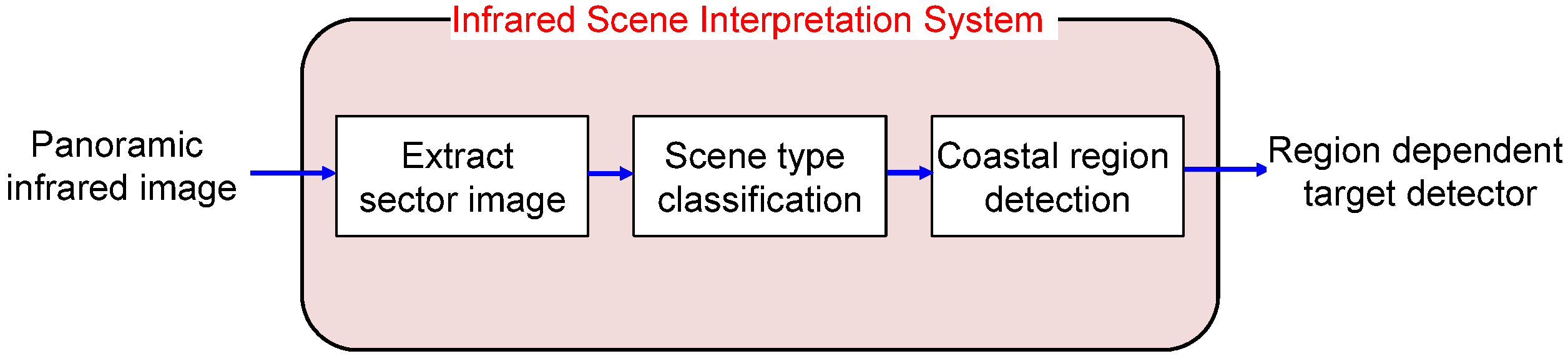
2. Proposed Infrared Scene Interpretation System

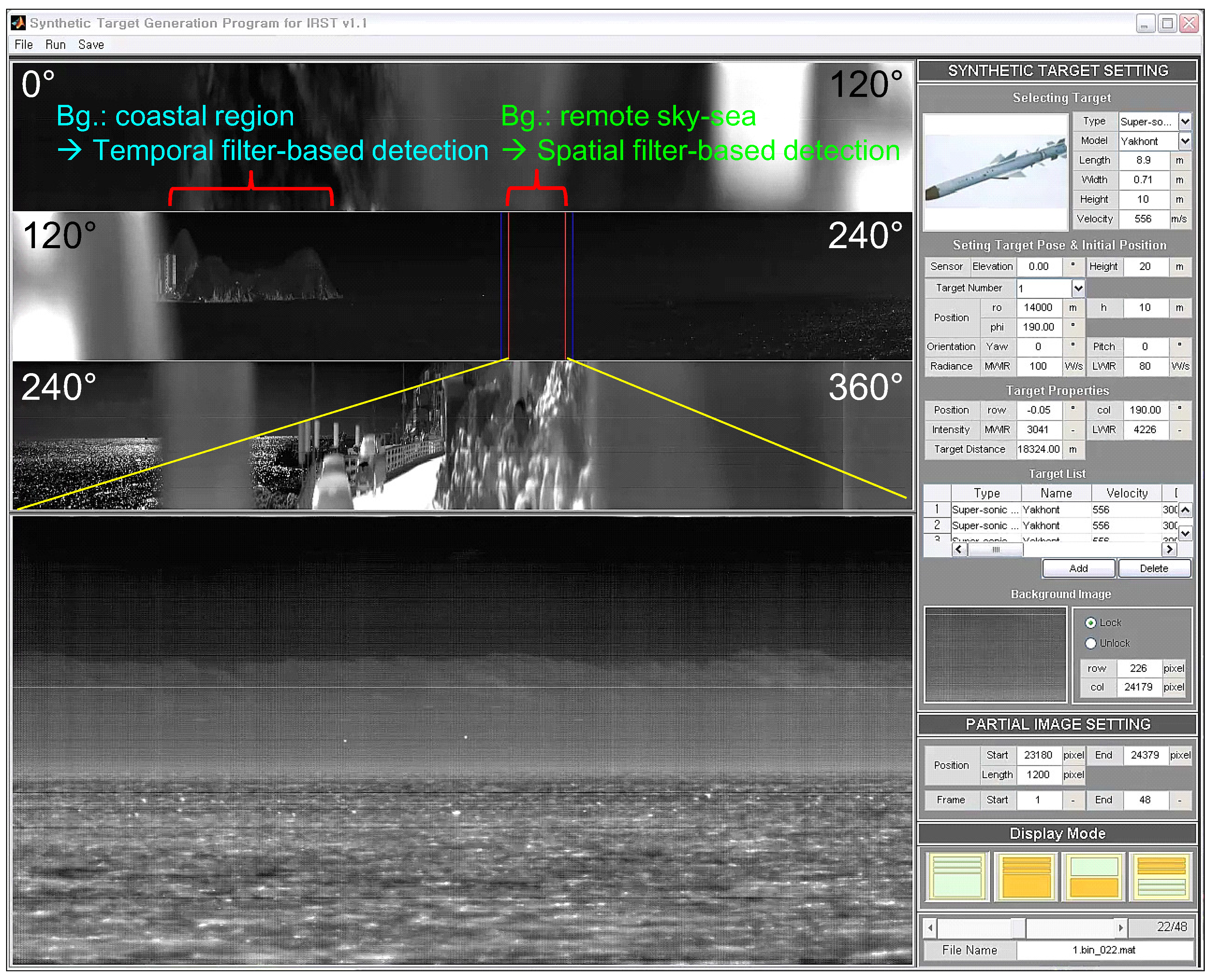
2.1. Properties of the Sea-Based IRST Background
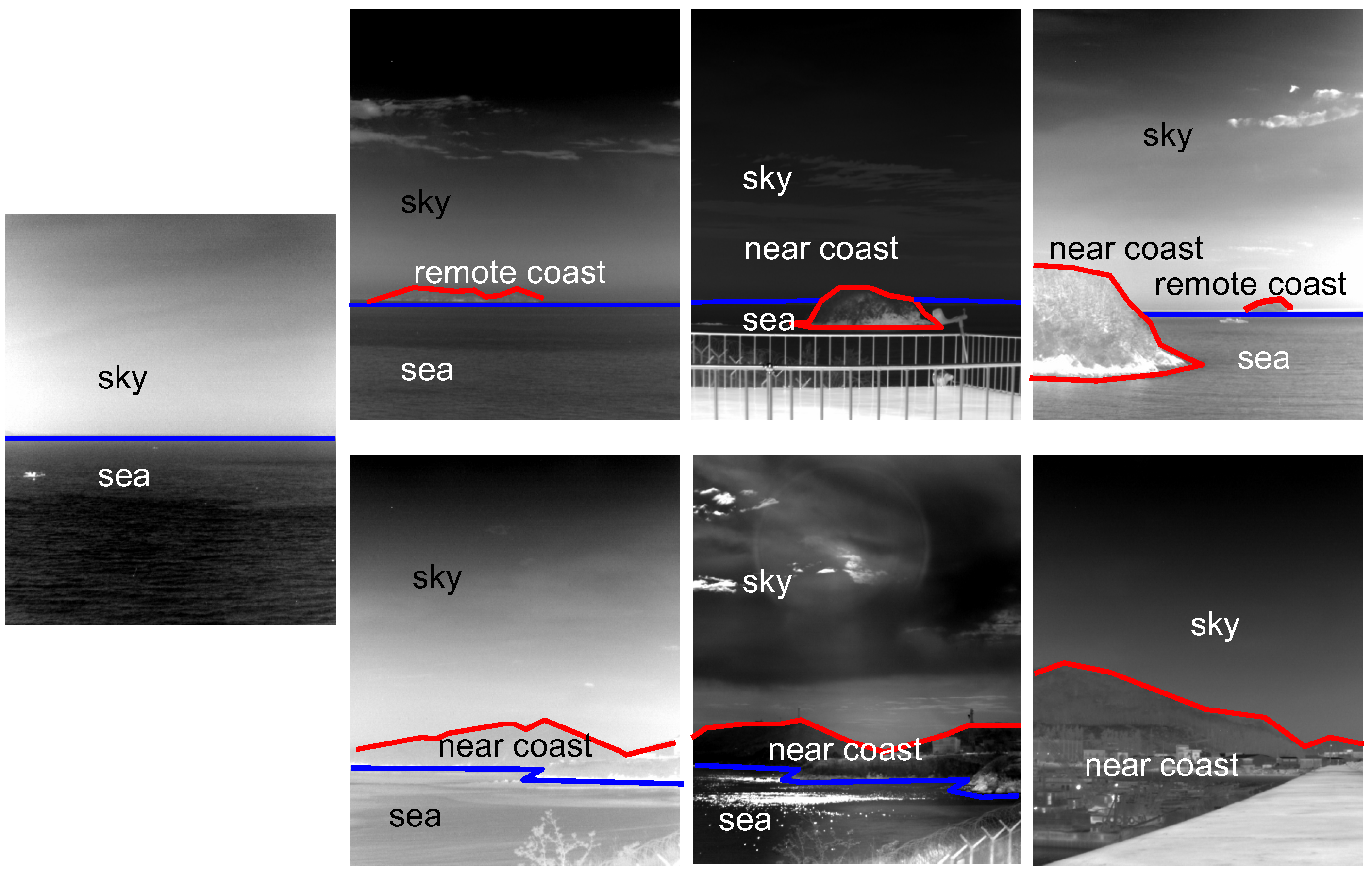
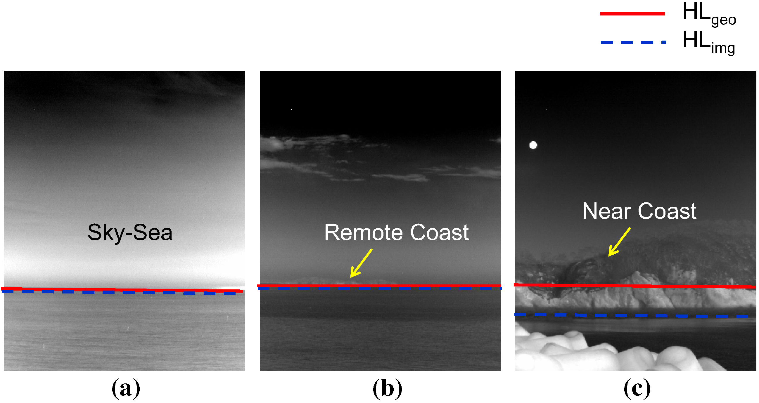
- The shapes of the sky, coast and sea regions are wide, because the imaging view point is slanted.
- The order of the background is predictable, such as sky-sea, sky-coast-sea and sky-coast. The reverse order is not permitted.
- A lower coast region generally occludes other remote regions due to the geometry of the camera projection.


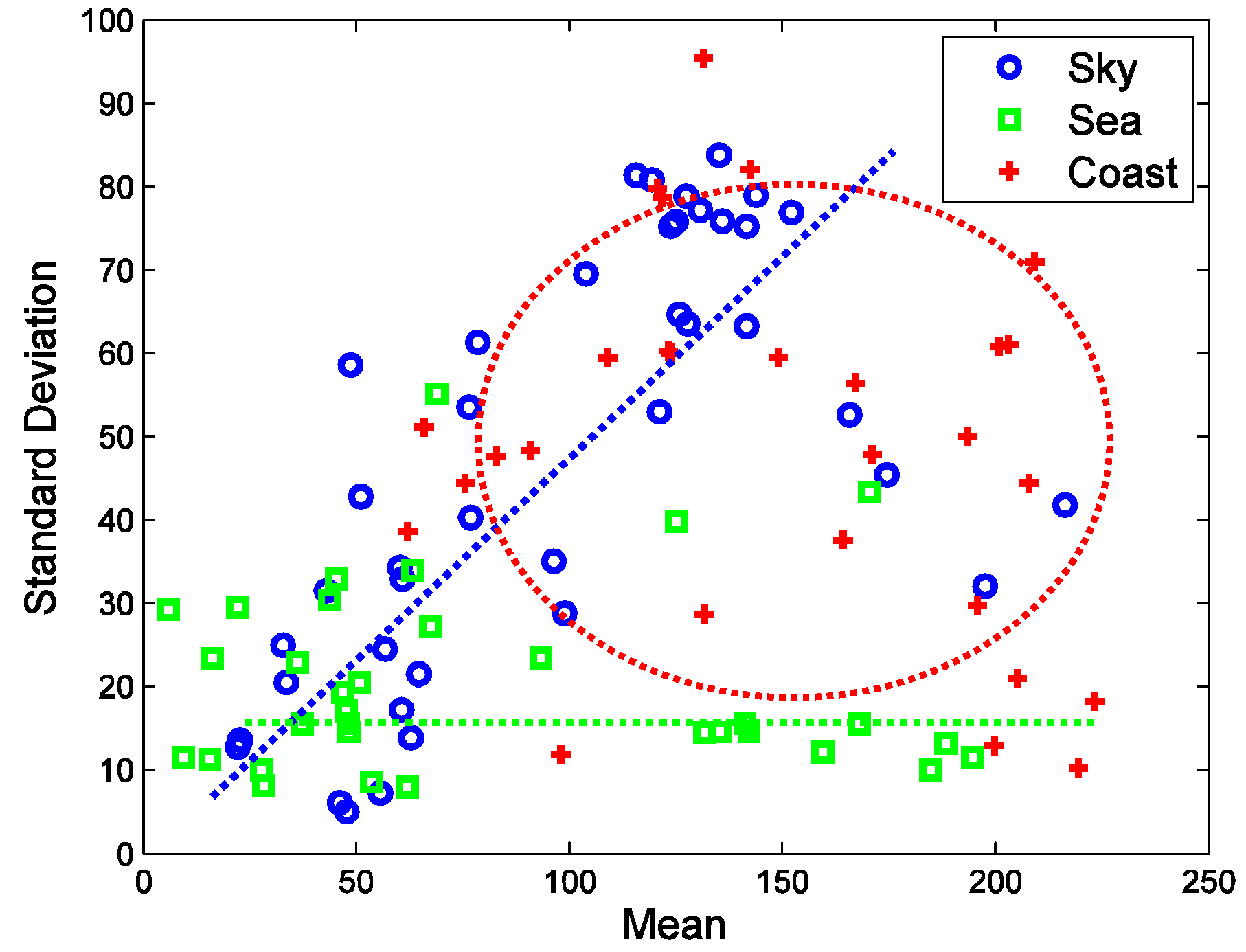
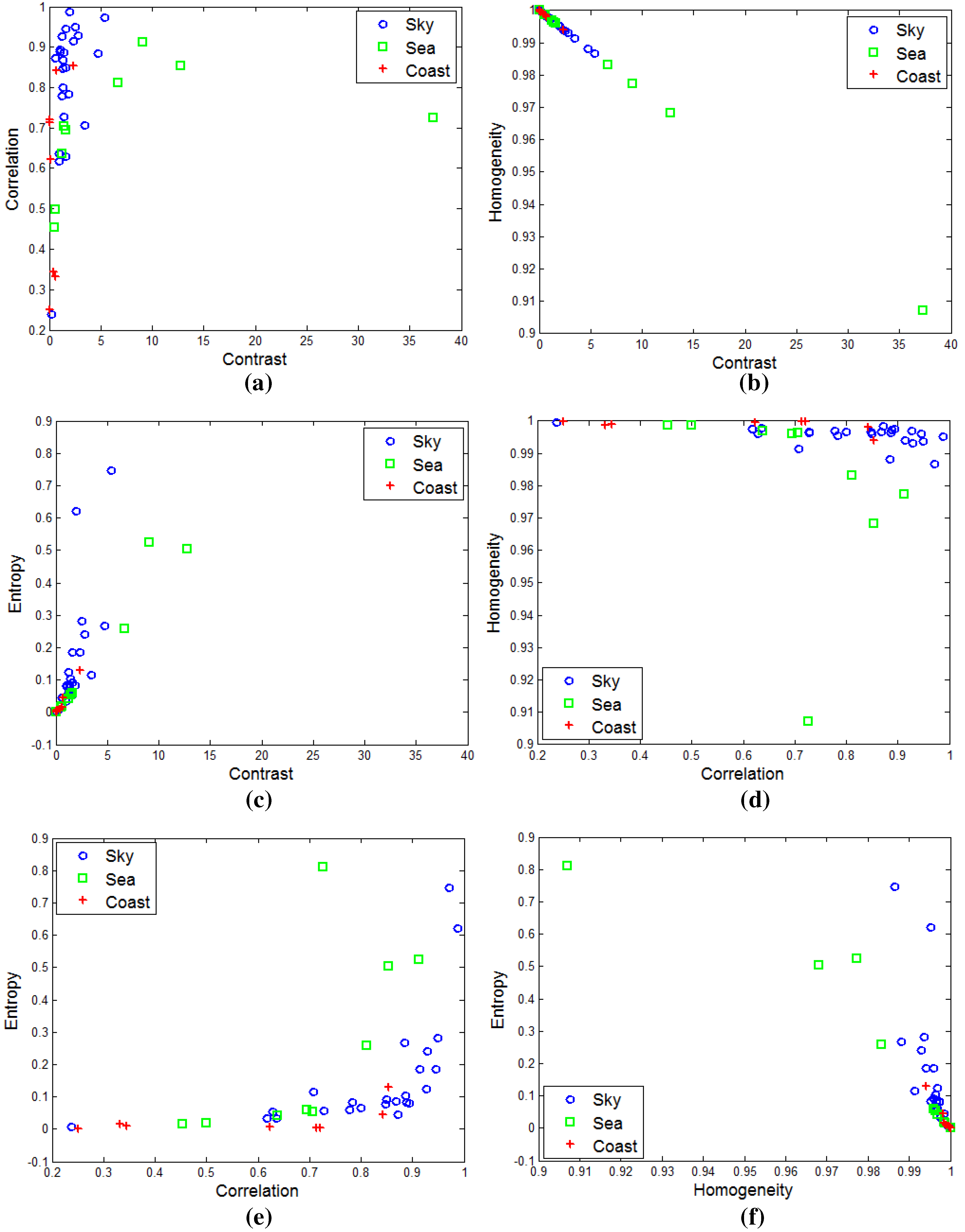
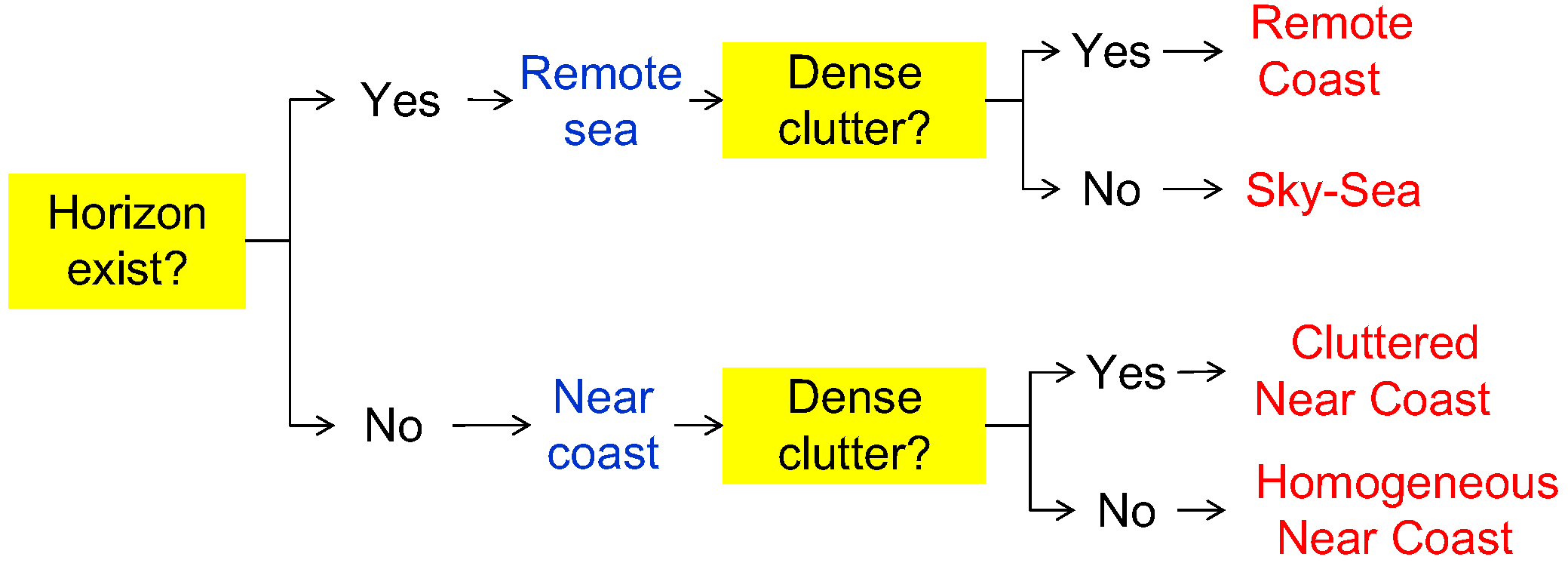
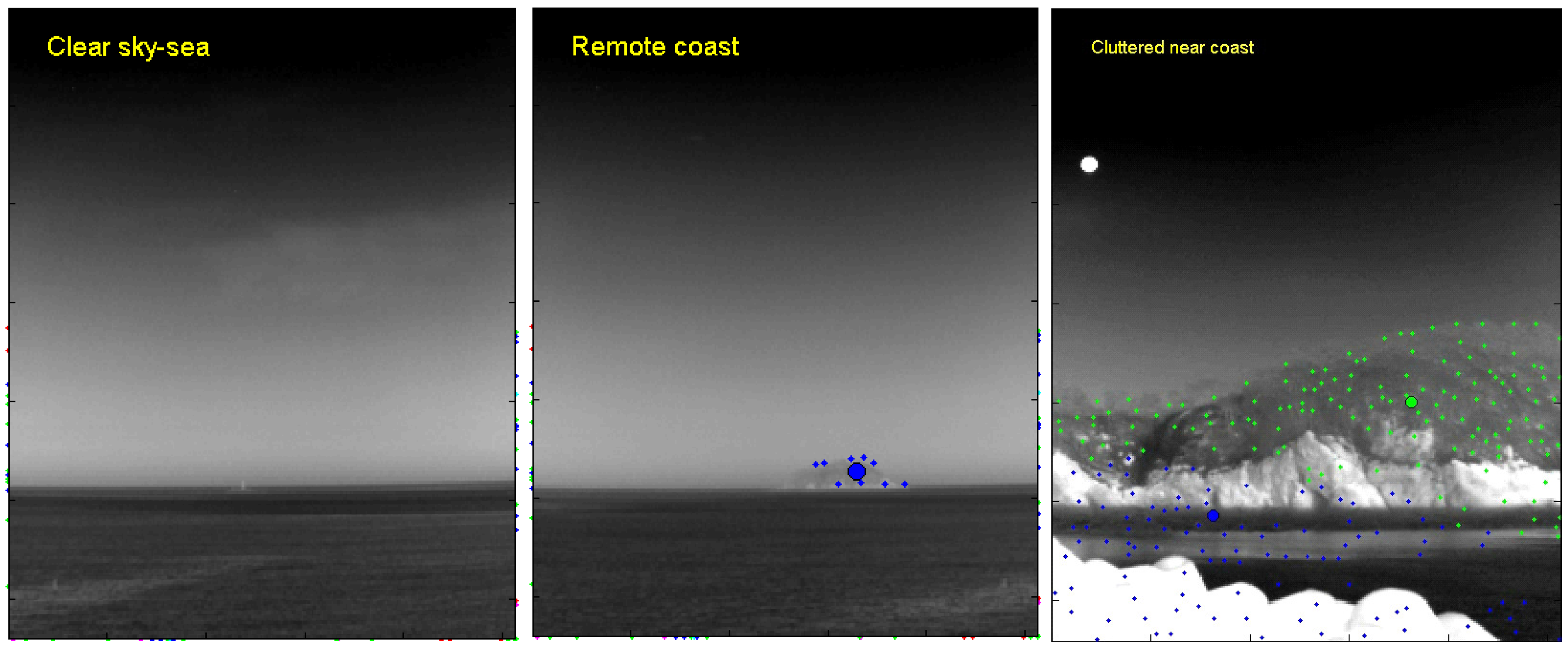
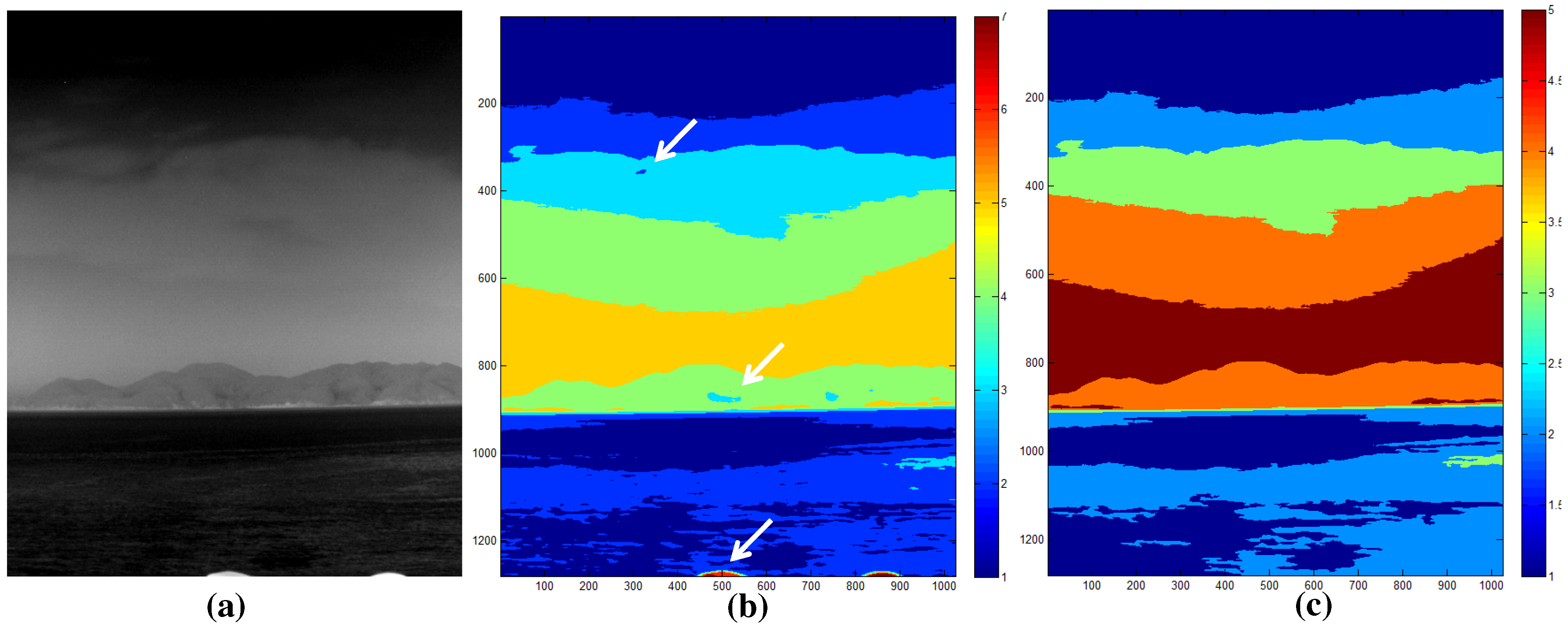
2.2. Infrared Background Type Classification


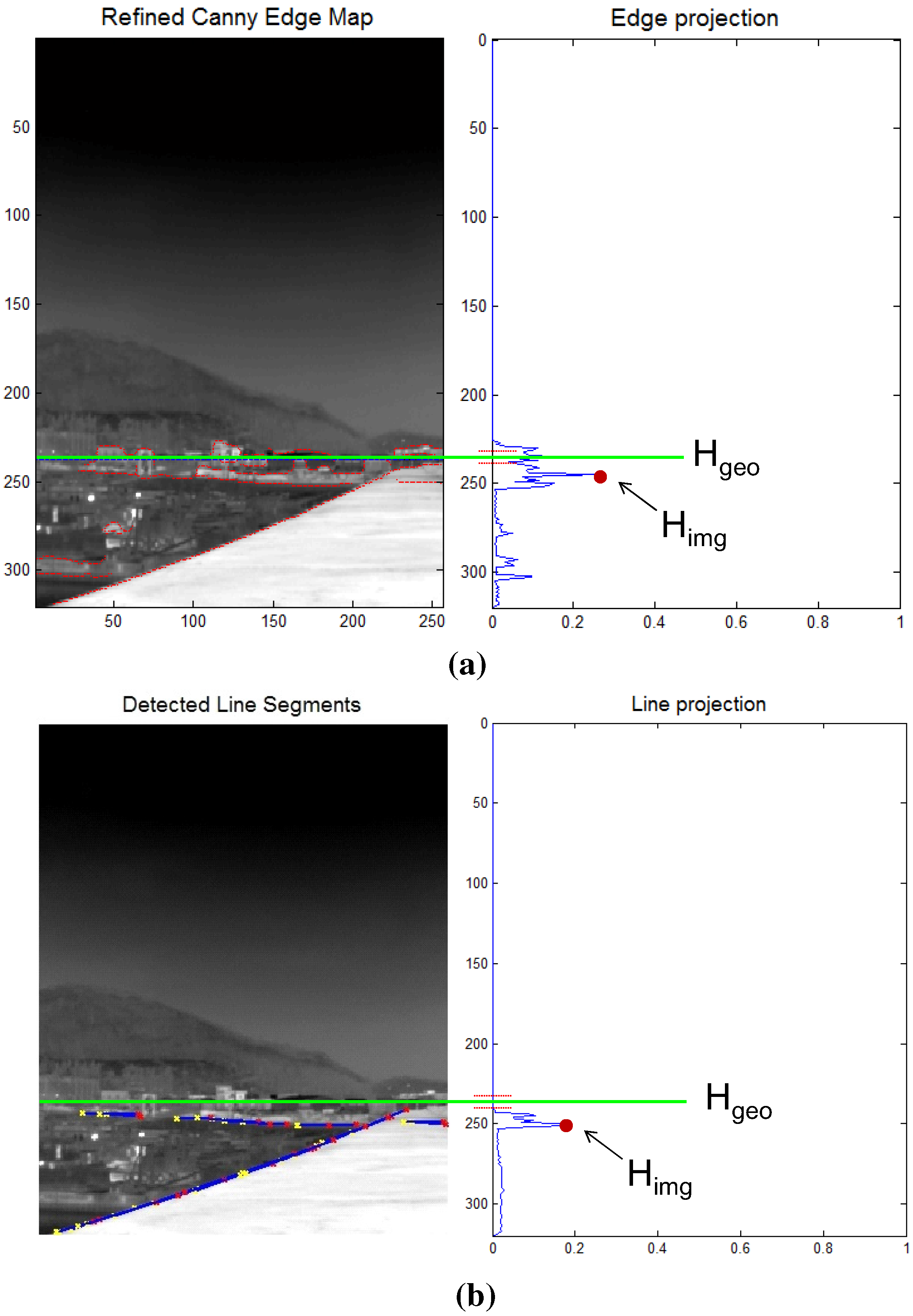
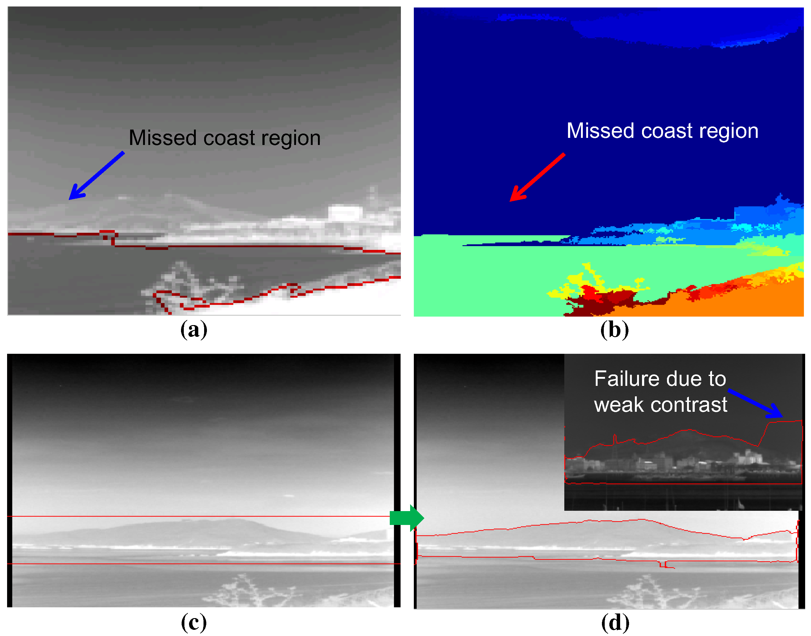
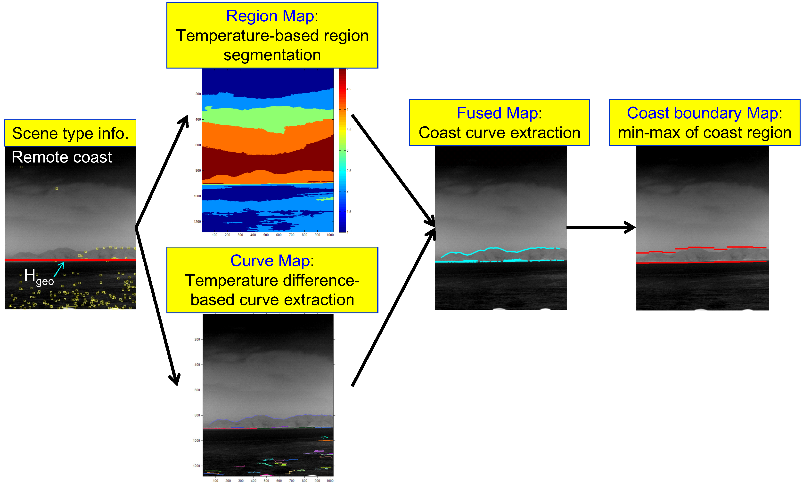
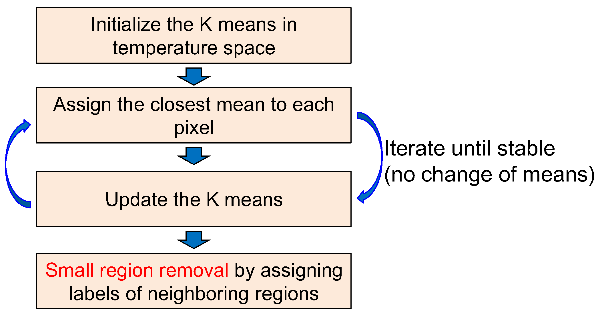
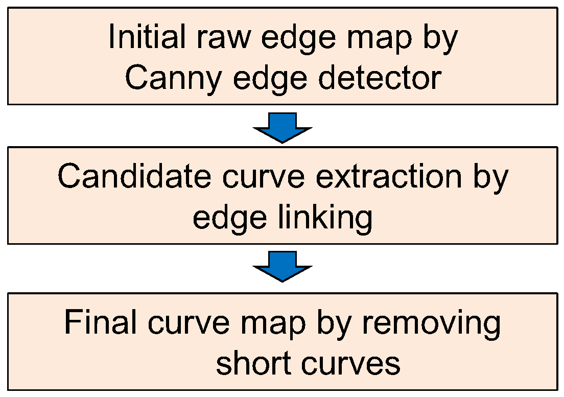
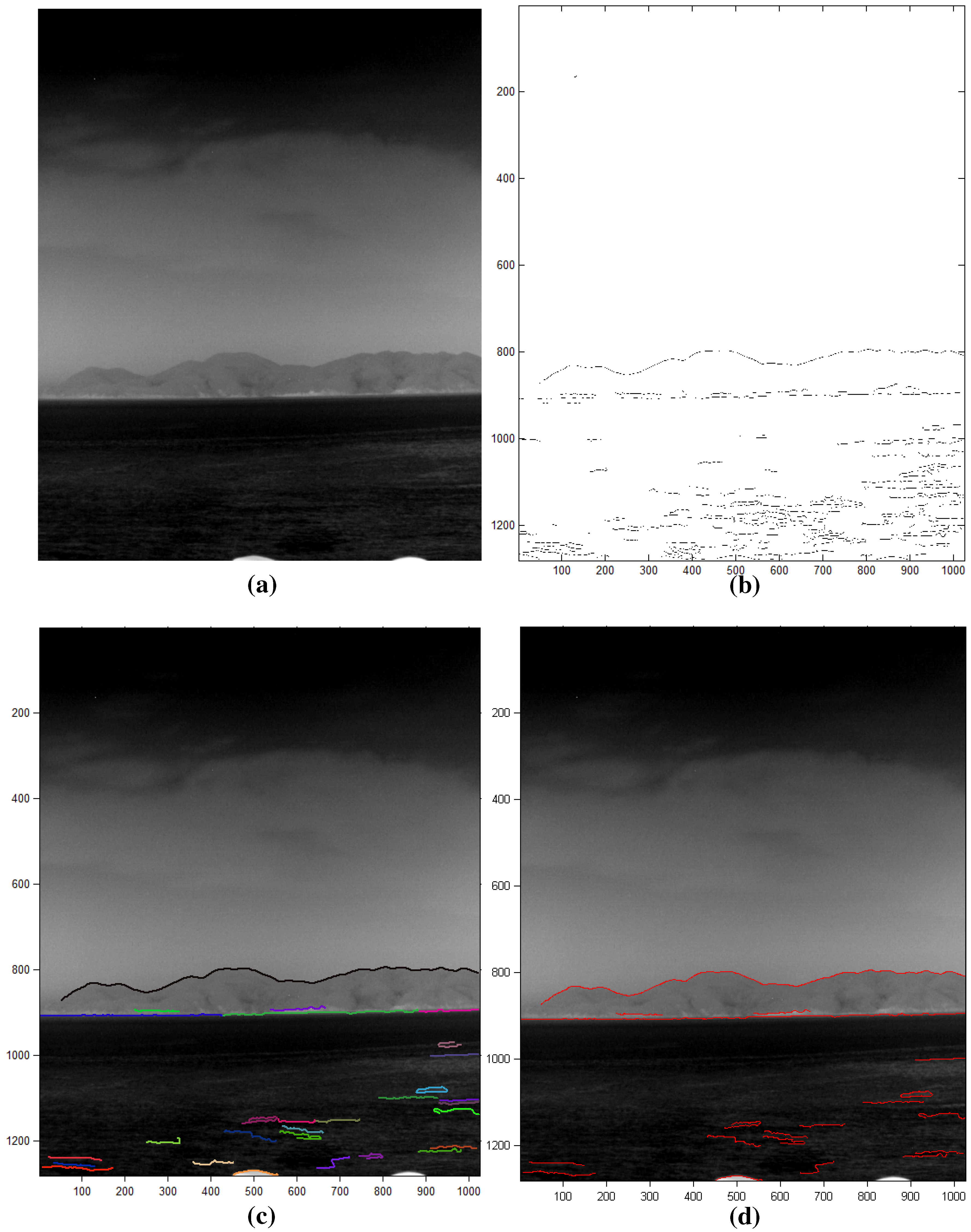
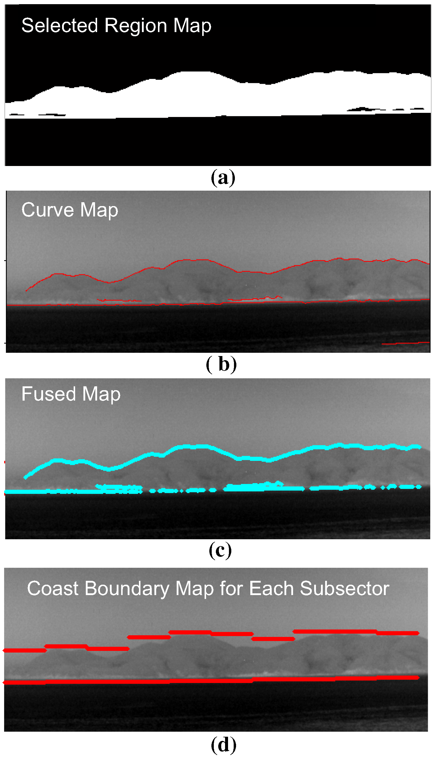
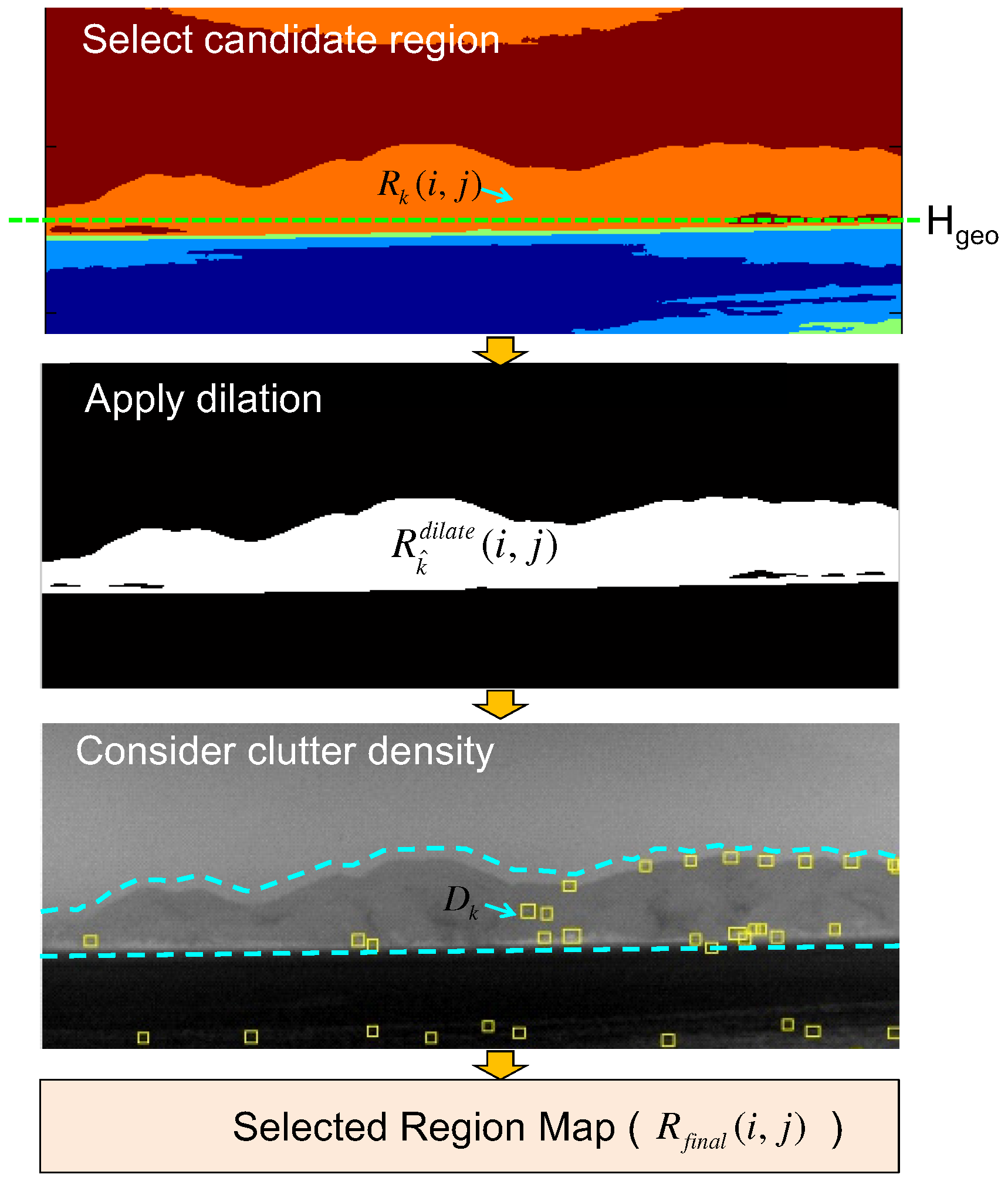
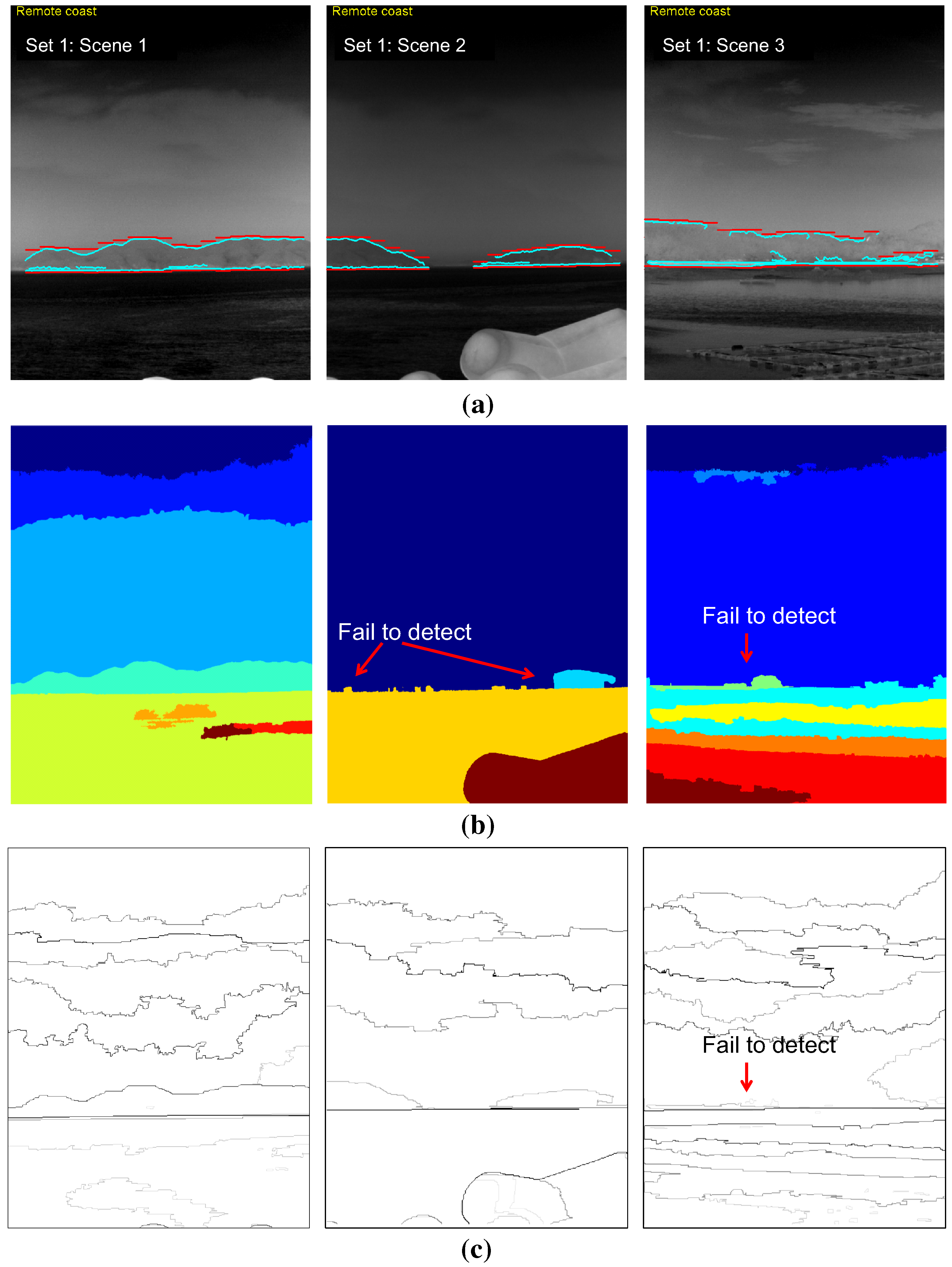
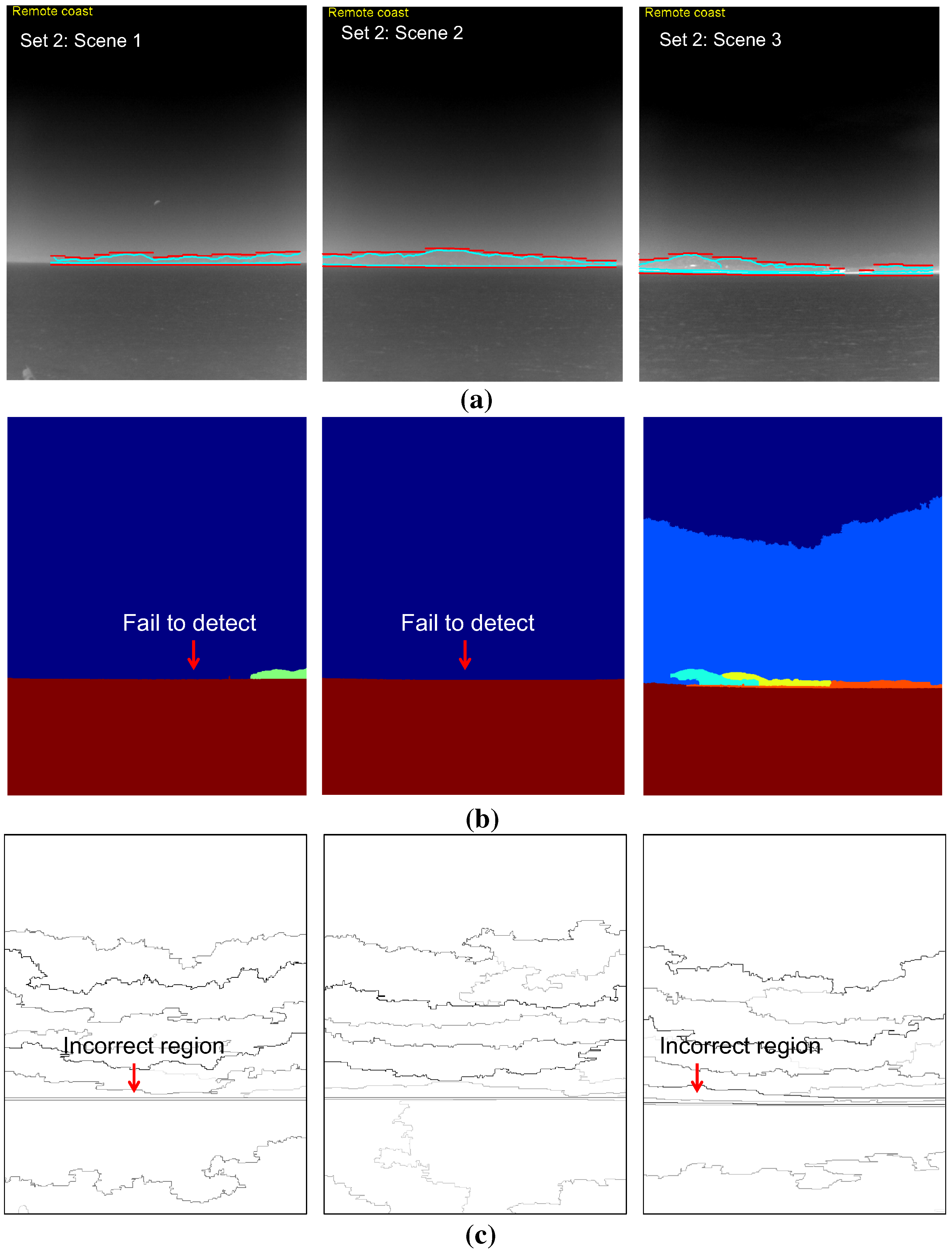
2.3. Coastal Region Detection


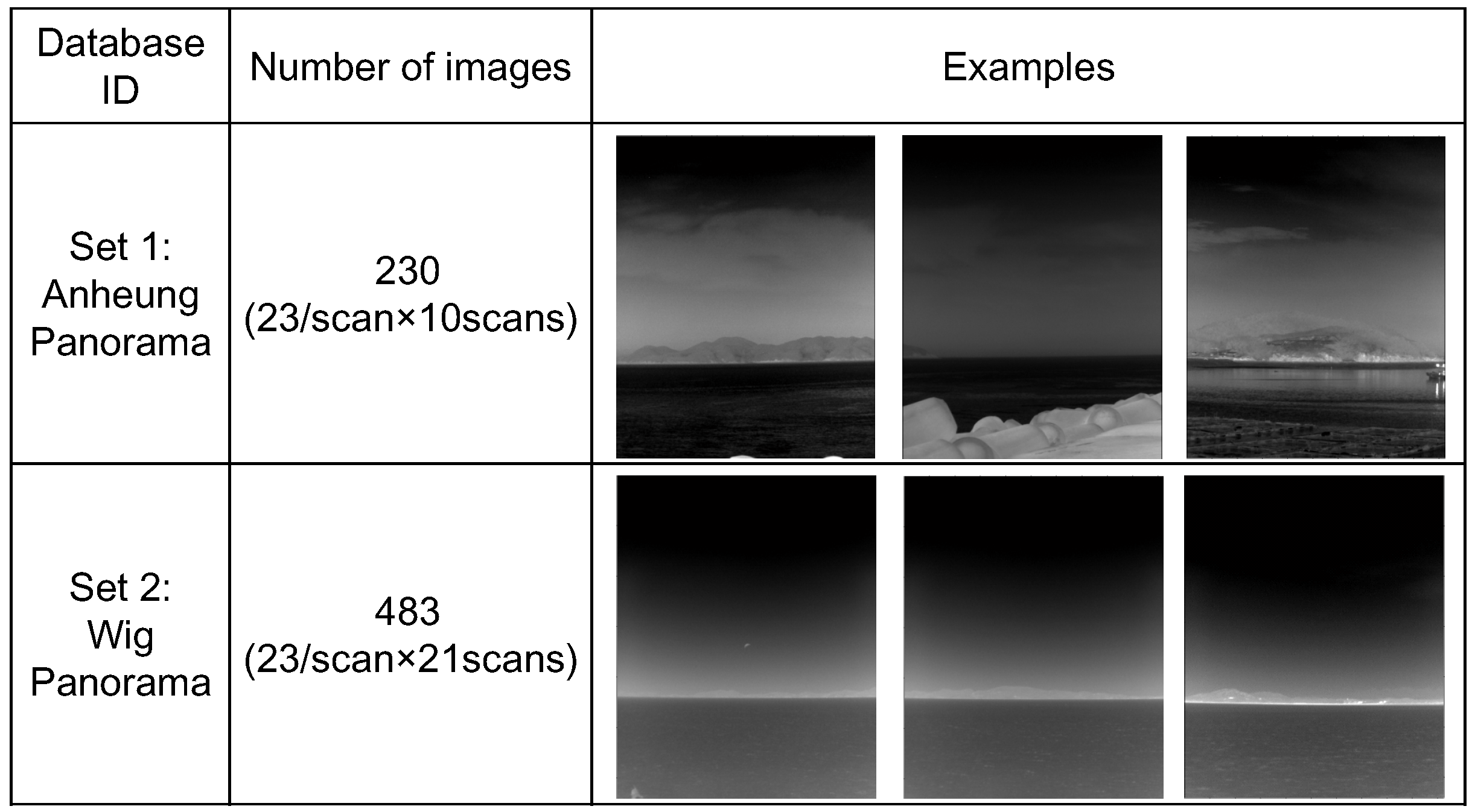
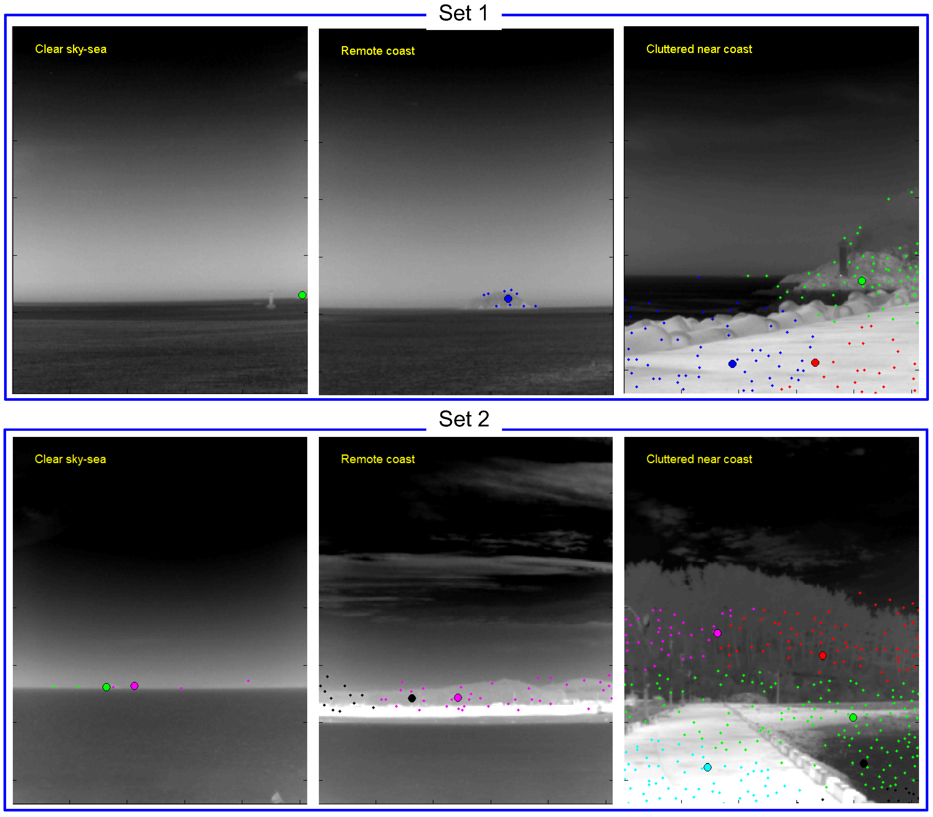
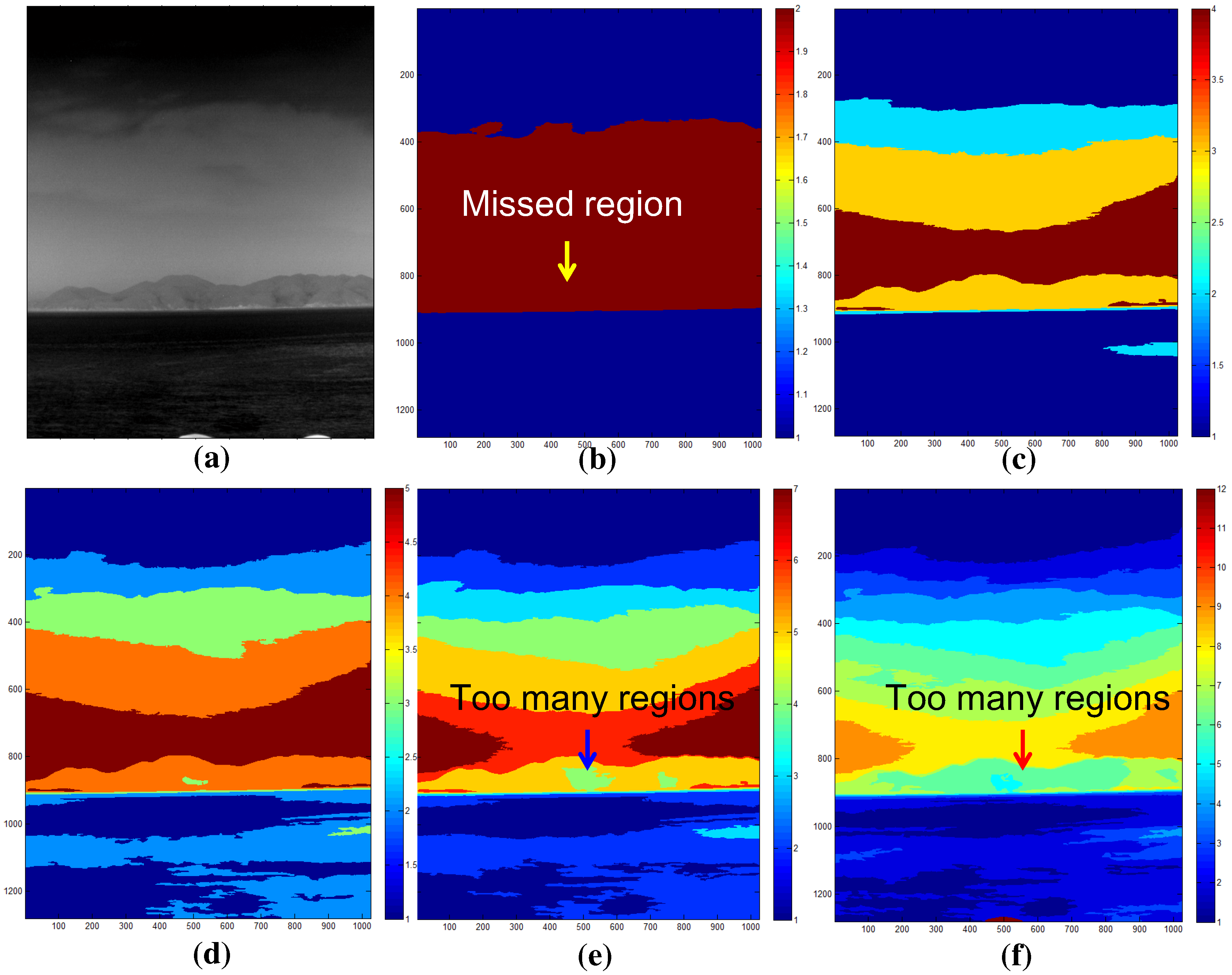
3. Experimental Results


| Dataset | Sky-Sea | Cluttered Remote Coast | Cluttered Near Coast | Accuracy (%) |
|---|---|---|---|---|
| Set 1 | 60/60 | 60/60 | 100/110 | 95.6% (220/230) |
| Set 2 | 42/42 | 294/315 | 126/126 | 95.7% (463/484) |


| Test scene | Proposed | Mean-Shift Segmentation [28] | Statistical Region Mergin [35] | |||
|---|---|---|---|---|---|---|
| DR [%] | DR [%] | DR [%] | ||||
| Set 1:Scene 1 | 19/19 | 100% | 19/19 | 100% | 19/19 | 100% |
| Set 1:Scene 2 | 19/19 | 100% | 2/19 | 10.5% | 19/19 | 100% |
| Set 1:Scene 3 | 16/19 | 84.2% | 0/19 | 0% | 0/19 | 0% |
| Set 2:Scene 1 | 17/17 | 100% | 2/17 | 11.8% | 0/19 | 0% |
| Set 2:Scene 2 | 19/19 | 100% | 0/19 | 0% | 19/19 | 100% |
| Set 2:Scene 3 | 18/19 | 94.7% | 16/19 | 84.2% | 17/19 | 89.4% |
| Overall | 108/112 | 96.4% | 39/112 | 34.8% | 74/112 | 66.0% |


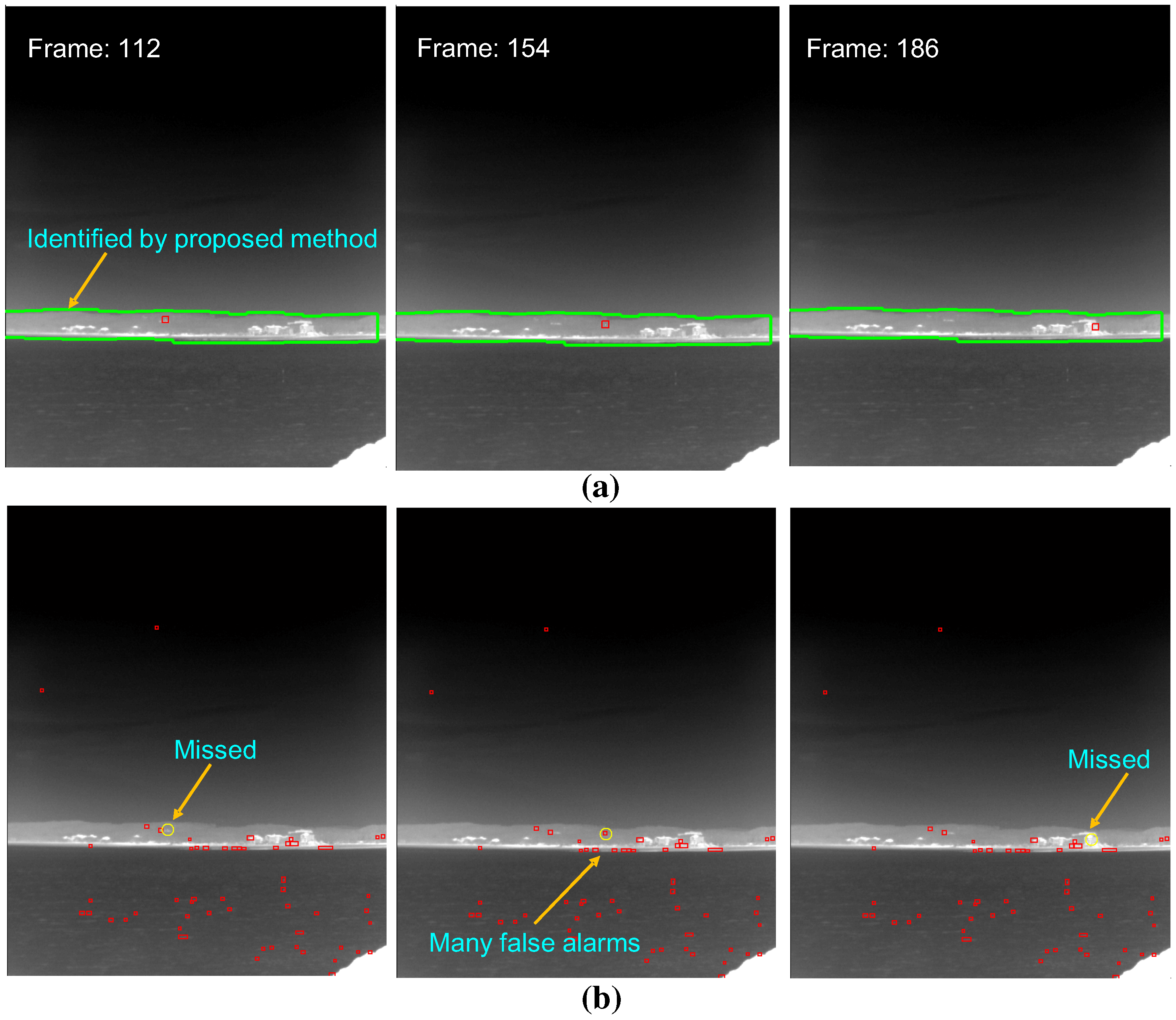
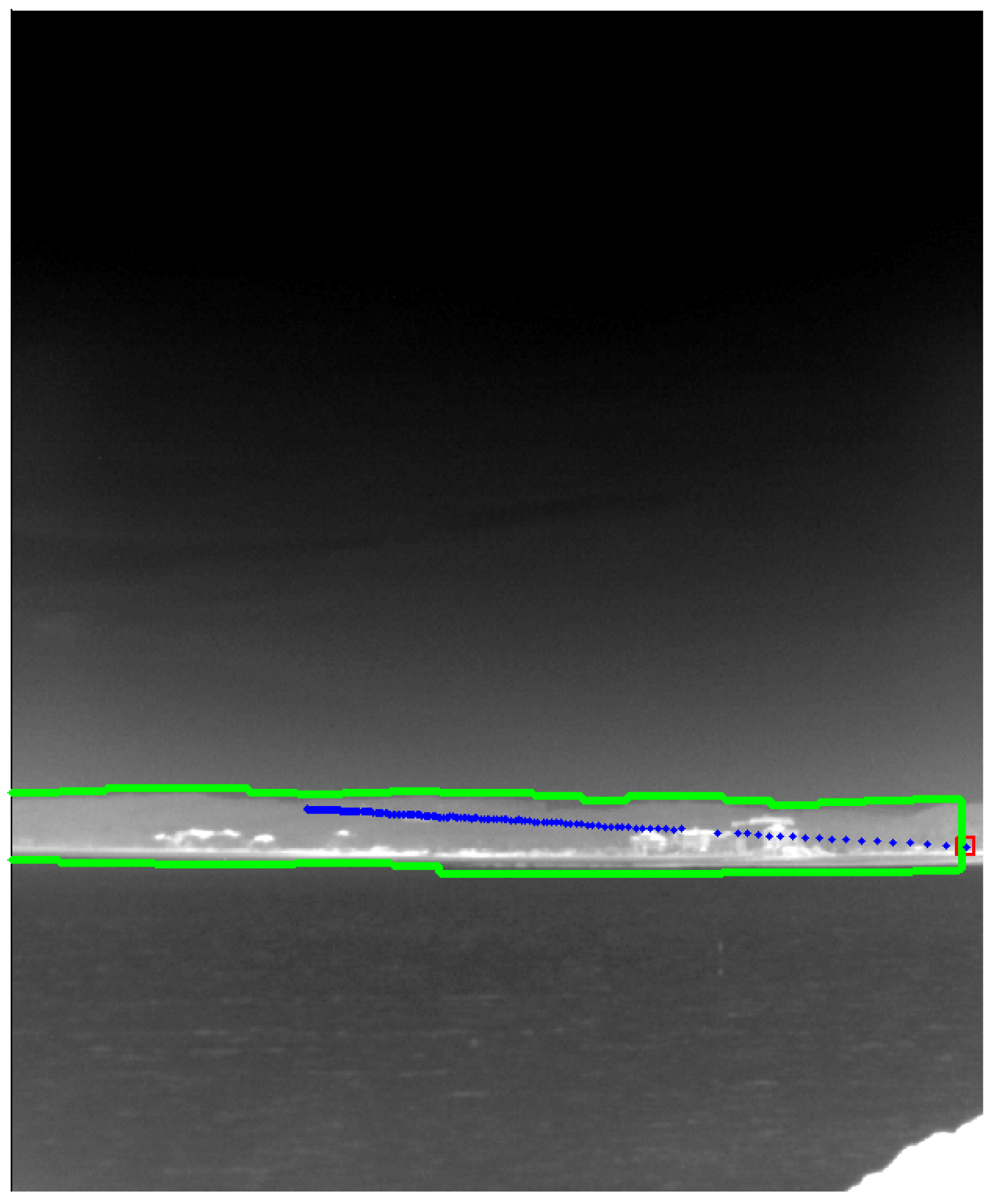
| DB Types | Performance Measure | With Coast Information by the Proposed Method Temporal Filter (TCF [37]) | Without Coast Information Spatial Filter (Top-Hat [5]) |
|---|---|---|---|
| Synthetic | Detection rate | 97.7% (171/175) | 89.7% (157/175) |
| DB | FAR | 0/image | 54/image |
| WIGcraft | Detection rate | 98.3% (60/61) | 85.3% (52/61) |
| DB | FAR | 0/image | 65/image |


4. Conclusions and Discussion
Acknowledgments
Author Contributions
Conflicts of Interest
References
- De Jong, A.N. IRST and perspective. Proc. SPIE 1995, 2552, 206–213. [Google Scholar]
- Ristic, B.; Hernandez, M.; Farina, A.; Hwa-Tung, O. Analysis of radar allocation requirements for an IRST aided tracking of anti-ship missiles. In Proceedings of the 9th International Conference on Information Fusion, Florence, Italy, 10–13 July 2006; pp. 1–8.
- Sang, H.; Shen, X.; Chen, C. Architecture of a configurable 2-D adaptive filter used for small object detection and digital image processing. Opt. Eng. 2003, 48, 2182–2189. [Google Scholar] [CrossRef]
- Warren, R.C. Detection of Distant Airborne Targets in Cluttered Backgrounds in Infrared Image Sequences. Ph.D. Thesis, University of South Australia, Adelaide, Australia, 2002. [Google Scholar]
- Wang, Y.L.; Dai, J.M.; Sun, X.G.; Wang, Q. An efficient method of small targets detection in low SNR. J. Phys. Conf. Ser. 2006, 48, 427–430. [Google Scholar] [CrossRef]
- Rozovskii, B.; Petrov, A. Optimal Nonlinear Filtering for Track-before-Detect in IR Image Sequences. Proc. SPIE 1999, 3809, 152–163. [Google Scholar]
- Thiam, E.; Shue, L.; Venkateswarlu, R. Adaptive Mean and Variance Filter for Detection of Dim Point-Like Targets. Proc. SPIE 2002, 4728, 492–502. [Google Scholar]
- Zhang, Z.; Cao, Z.; Zhang, T.; Yan, L. Real-time detecting system for infrared small target. Proc. SPIE 2007, 6786. [Google Scholar] [CrossRef]
- Kim, S.; Sun, S.G.; Kim, K.T. Highly efficient supersonic small infrared target detection using temporal contrast filter. Electron. Lett. 2014, 50, 81–83. [Google Scholar] [CrossRef]
- Sang, N.; Zhang, T.; Shi, W. Detection of Sea Surface Small Targets in Infrared Images based on Multi-level Filters. Proc. SPIE 1998, 3373, 123–129. [Google Scholar]
- Chan, D.S.K. A Unified Framework for IR Target Detection and Tracking. Proc. SPIE 1992, 1698, 66–76. [Google Scholar]
- Tzannes, A.P.; Brooks, D.H. Point Target Detection in IR Image Sequences: A Hypothesis-Testing Approach based on Target and Clutter Temporal Profile Modeling. Opt. Eng. 2000, 39, 2270–2278. [Google Scholar]
- Schwering, P.B.; van den Broek, S.P.; van Iersel, M. EO System Concepts in the Littoral. Proc. SPIE 2007, 6542. [Google Scholar] [CrossRef]
- Wong, W.-K.; Chew, Z.-Y.; Lim, H.-L.; Loo, C.-K.; Lim, W.-S. Omnidirectional Thermal Imaging Surveillance System Featuring Trespasser and Faint Detection. Int. J. Image Proc. 2011, 4, 518–538. [Google Scholar]
- Missirian, J.M.; Ducruet, L. IRST: A key system in modern warfare. Proc. SPIE 1997, 3061, 554–565. [Google Scholar]
- Grollet, C.; Klein, Y.; Megaides, V. ARTEMIS: Staring IRST for the FREMM frigate. Proc. SPIE 2007, 6542. [Google Scholar] [CrossRef]
- Fontanella, J.C.; Delacourt, D.; Klein, Y. ARTEMIS: First naval staring IRST in service. Proc. SPIE 2010, 7660. [Google Scholar] [CrossRef]
- Weihua, W.; Zhijun, L.; Jing, L.; Yan, H.; Zengping, C. A Real-time Target Detection Algorithm for Panorama Infrared Search and Track System. Procedia Eng. 2012, 29, 1201–1207. [Google Scholar] [CrossRef]
- Dijk, J.; van Eekeren, A.W.M.; Schutte, K.; de Lange, D.J.J. Point target detection using super-resolution reconstruction. Proc. SPIE 2007, 6566. [Google Scholar] [CrossRef]
- Kim, S. Min-local-LoG filter for detecting small targets in cluttered background. Electron. Lett. 2011, 47, 105–106. [Google Scholar] [CrossRef]
- Kim, S.; Lee, J. Scale invariant small target detection by optimizing signal-to-clutter ratio in heterogeneous background for infrared search and track. Pattern Recognit. 2012, 45, 393–406. [Google Scholar] [CrossRef]
- Kim, S.; Sun, S.G.; Kwon, S.; Kim, K.T. Robust coastal region detection method using image segmentation and sensor LOS information for infrared search and track. Proc. SPIE 2013, 8744. [Google Scholar] [CrossRef]
- Blanton, W.B.; Barner, K.E. Infrared Region Classification using Texture and Model-based Features. In Proceedings of the IEEE International Conference on Acoustics, Speech and Signal Processing (ICASSP), Las Vegas, NV, USA, 31 March–4 April 2008; pp. 1329–1332.
- Kim, S.; Lee, J. Small Infrared Target Detection by Region-Adaptive Clutter Rejection for Sea-Based Infrared Search and Track. Sensors 2014, 2014, 13210–13242. [Google Scholar] [CrossRef] [PubMed]
- Zhou, P.; Ye, W.; Wang, Q. An Improved Canny Algorithm for Edge Detection. J. Comput. Inf. Syst. 2011, 7, 1516–1523. [Google Scholar]
- Fernandes, L.; Oliveira, M. Real-time line detection through an improved Hough transform voting scheme. Pattern Recognit. 2007, 41, 299–314. [Google Scholar] [CrossRef]
- Richter, R.; Davis, J.S.; Duggin, M.J. Radiometric sensor performance model including atmospheric and IR clutter effects. Proc. SPIE 1997, 3062. [Google Scholar] [CrossRef]
- Comaniciu, D.; Meer, P. Mean Shift: A Robust Approach Toward Feature Space Analysis. IEEE Trans. Pattern Anal. Mach. Intell. 2002, 24, 603–619. [Google Scholar] [CrossRef]
- Shi, J.; Malik, J. Normalized Cuts and Image Segmentation. IEEE Trans. Pattern Anal. Mach. Intell. 2000, 22, 888–905. [Google Scholar]
- Xu, C.; Prince, J.L. Snakes, Shapes, and Gradient Vector Flow. IEEE Trans. Image Proc. 1998, 7, 359–369. [Google Scholar]
- Yao, H.; Duan, Q.; Li, D.; Wang, J. An improved K-means clustering algorithm for fish image segmentation. Math. Comput. Model. 2013, 58, 790–798. [Google Scholar] [CrossRef]
- Gonzalez, R.; Woods, R. Digital Image Processing, 3rd ed.; Prentice Hall: Saddle River, NJ, USA, 2008. [Google Scholar]
- Klein, L.A. Sensor and Data Fusion Concepts and Applications, 2nd ed.; SPIE Press: Bellingham, WA, USA, 1999. [Google Scholar]
- Mikolajczyk, K.; Tuytelaars, T.; Schmid, C.; Zisserman, A.; Matas, J.; Schaffalitzky, F.; Kadir, T.; Gool, L.V. A Comparison of Affine Region Detectors. Int. J. Comput. Vis. 2005, 65, 43–72. [Google Scholar] [CrossRef]
- Nock, R.; Nielsen, F. Statistical Region Merging. IEEE Trans. Pattern Anal. Mach. Intell. 2004, 26, 1452–1458. [Google Scholar] [CrossRef] [PubMed]
- Kim, S.; Yang, Y.; Choi, B. Realistic infrared sequence generation by physics-based infrared target modeling for infrared search and track. Opt. Eng. 2010, 49. [Google Scholar] [CrossRef]
- Kim, S. High-speed incoming infrared target detection by fusion of spatial and temporal detectors. Sensors 2015, 15, 7267–7293. [Google Scholar] [CrossRef] [PubMed]
© 2015 by the author; licensee MDPI, Basel, Switzerland. This article is an open access article distributed under the terms and conditions of the Creative Commons Attribution license (http://creativecommons.org/licenses/by/4.0/).
Share and Cite
Kim, S. Sea-Based Infrared Scene Interpretation by Background Type Classification and Coastal Region Detection for Small Target Detection. Sensors 2015, 15, 24487-24513. https://doi.org/10.3390/s150924487
Kim S. Sea-Based Infrared Scene Interpretation by Background Type Classification and Coastal Region Detection for Small Target Detection. Sensors. 2015; 15(9):24487-24513. https://doi.org/10.3390/s150924487
Chicago/Turabian StyleKim, Sungho. 2015. "Sea-Based Infrared Scene Interpretation by Background Type Classification and Coastal Region Detection for Small Target Detection" Sensors 15, no. 9: 24487-24513. https://doi.org/10.3390/s150924487
APA StyleKim, S. (2015). Sea-Based Infrared Scene Interpretation by Background Type Classification and Coastal Region Detection for Small Target Detection. Sensors, 15(9), 24487-24513. https://doi.org/10.3390/s150924487