3.1. Experimental Setup
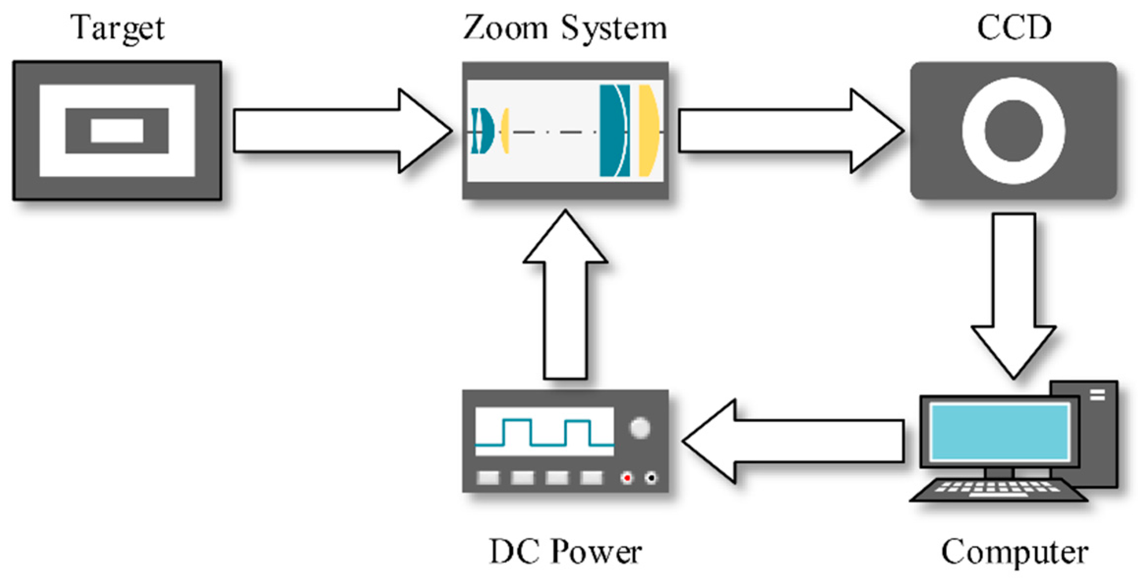
In order to test the performance of the zoom system, we set up an experimental platform shown in
Figure 6. Test targets were backlit with white light and two forms of targets were used in measurement. The size of the target was 240 mm × 170 mm. The zoom system was placed between the test target and the CCD camera, and the object distance was set to be 265 mm. The CCD was 1/4 inch, pixel size of which was 7.4 μm. In fact, the zoom system and the CCD camera were fixed connected through a standard C lens mount. CCD camera captured the images and then sent them to the computer. We obtained the information on imaging quality and magnification through image processing, and then sent new control parameters to the zoom system. A dc power supply was used to complete the D/A conversion.
Figure 6.
Structure of the experimental platform.
Figure 6.
Structure of the experimental platform.
There were two major parameters we needed to measure: EFL and modulation transfer function (MTF). EFL was used to evaluate the zoom ratio and zoom precision, and MTF was used to evaluate the imaging quality. During measurement, we selected 20 sampling points as we had done in simulation when adjusted I2 from 5 mA to 100 mA. The forms of targets and the methods of measuring EFL and MTF would be discussed in the following sections.
3.2. Initial Structure
In their initial state, I
1 and I
2 both took 0 mA. MTF was used to evaluate the quality of imaging. The method of calculating MTF of the system would be provided in
Section 3.6, we currently used the calculation result. Initial parameters of the zoom system are shown in
Table 4. MTF value when spatial frequency took 20 lp/mm was used to evaluate the image quality.
Table 4.
Initial parameters of the zoom system.
Table 4.
Initial parameters of the zoom system.
| I2 (mA) | EFL (mm) | FOV (Degree) | MTF Value at 20l p/mm |
|---|
| 0 | 6.56 | 41.7 | 0.01 |
| 5 | 6.93 | 39.7 | 0.28 |
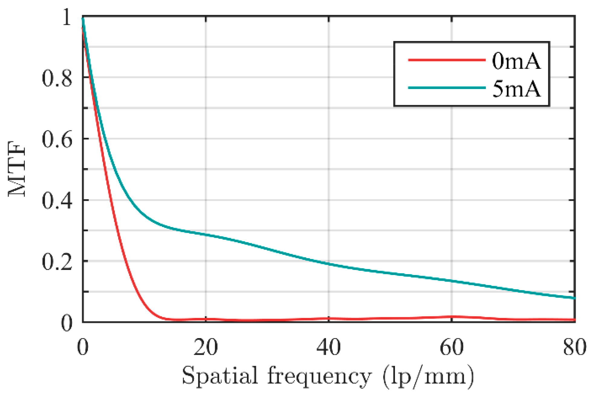
Image quality was poor because L1 had not compensated for L2 and the optical aberration of L2 was high when Φ4 took values near the limit position.
In order to achieve high image quality in the whole zoom process, we set I
2 = 5 mA and adjusted L
1 to compensate for L
2. MTF diagram is shown in
Figure 7. Parameters of the zoom system when I
2 takes 5 mA are shown in
Table 4.
Figure 7.
MTF curve of the zoom system when I2 took 0 mA and 5 mA, respectively.
Figure 7.
MTF curve of the zoom system when I2 took 0 mA and 5 mA, respectively.
In the following discussion, we take the state when I2 = 5 mA as the initial state.
3.3. Electrical Performance Testing
In the process of measuring, L2 was adjusted actively to change EFL of the zoom system when L1 supplied compensation to get clear images. The relationship between I1 and I2 can be calculated from Equations (1) and (2).
We set I
2 to a value, coarsely adjusted I
1 till we got clear image on computer, and then tightly adjusted I
1. Range of tight adjustment was usually less than ±4 mA in actual measurement. We could obtain the real-time MTF of the zoom system with the software written by ourselves on computer. In fact, the MTF curve had no obvious change when we adjusted I
1 in ±2 mA range. For I
1, this was an acceptable error range. Then we chose the value of MTF when spatial frequency was 20l p/mm as the image quality factor (Q). We considered the zoom system to achieve highest imaging quality when Q got maximum, and I
1 would be recorded. The results of simulation and measurement are shown in
Figure 8. Although there were differences between simulated curve and measured curve, we could easily obtain I
1 as function of I
2 by curve fitting. This enabled the zoom system to realize precise electric control. Both the simulated and the measured curves could be fitted well by three-order polynomials, and the correlation coefficients were larger than 0.999. This meant that we only needed a small amount of addition and multiplication operations to obtain I
1 by I
2.
Figure 8.
L1’s control current (I1) as function of L2’s control current (I2).
Figure 8.
L1’s control current (I1) as function of L2’s control current (I2).
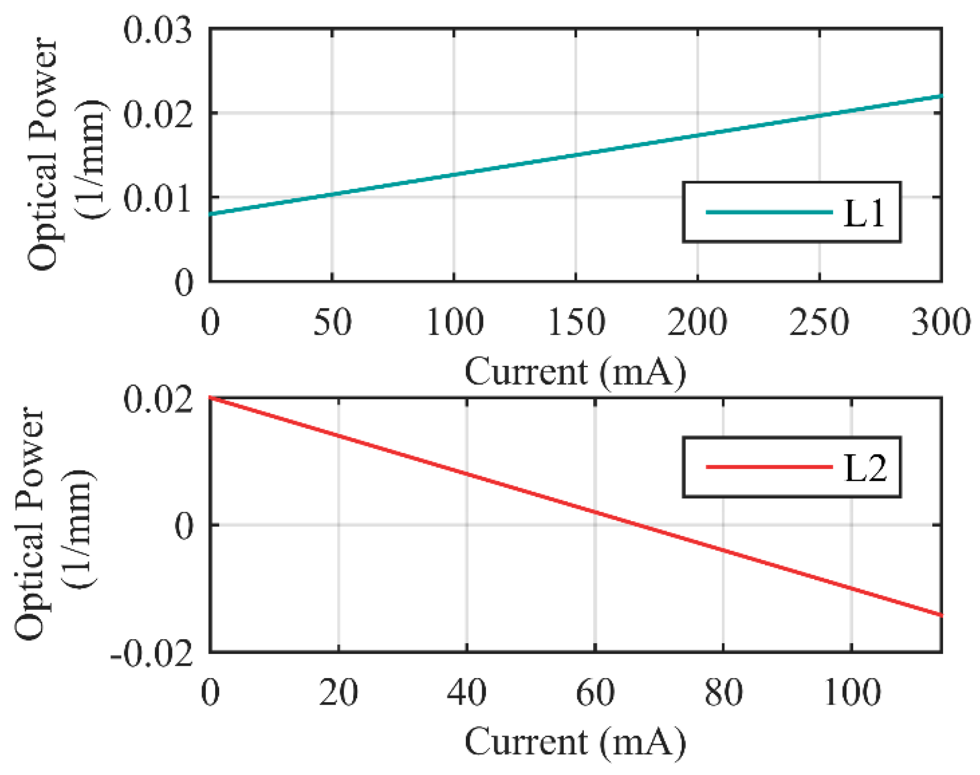
Optical power of the liquid lens was the only variant in the zoom system. Although in actual application on ground vehicle, it needed time to calculate I1 and I2 for specific EFL, the calculation time was usually at a microsecond level for most of the processors since there were only multiply and add operations in the fitting function. Therefore, the zoom speed depended only on the performance of the liquid lens. The response time of the system was less than 2.5 ms, and the settling time was less than 15 ms due to fluid viscosity.
3.4. Zoom Ratio Testing
Relationships between EFL, field of view (FOV), object height (OH), paraxial image height (PIH), and object distance (OD) could be obtained refer to Equations (5) and (6).
We obtained the magnification (m) of the zoom system by imaging a fixed length (lo) target. The magnification could be calculated refer to Equation (7) by counting the pixels (n) when the pixel size (μ) of the CCD camera was known.
Thus from Equations (5)−(7), we can obtain EFL refer to Equation (8).
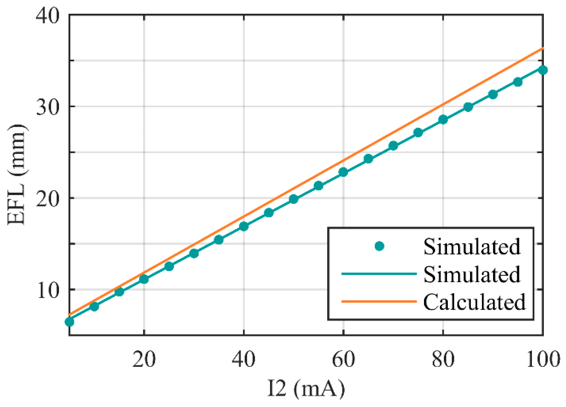
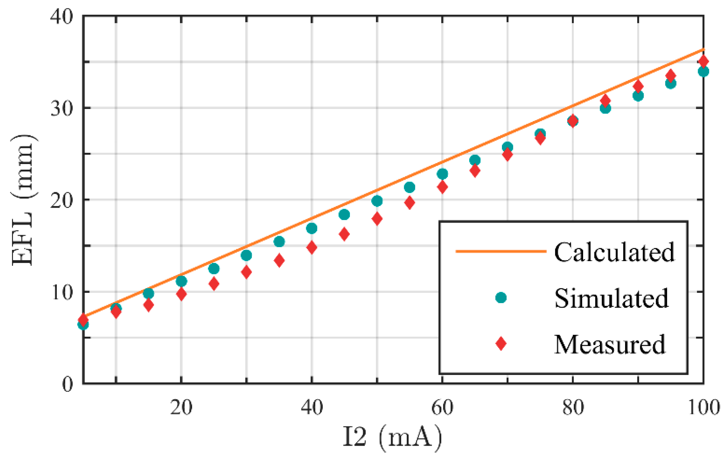
The measured and simulated results of EFLs are shown in
Table 5, and the EFL comparison diagram of calculated value, simulated value and measured value is shown in
Figure 9. An approximate linear relationship exists between EFL and I
2. Thus, we can easily determine I
2 to achieve specific EFL in actual application. As presented in
Section 3.3, I
1 could be calculated out by I
2 through the fitting function. Thus far, issues of determining control parameters to achieve specific EFL are completely solved.
Table 5.
Comparisons between simulated EFL and measured EFL.
Table 5.
Comparisons between simulated EFL and measured EFL.
| I2 (mA) | Simulated EFL (mm) | Measured EFL (mm) | Difference (mm) |
|---|
| 5 | 6.46 | 6.93 | 0.47 |
| 10 | 8.14 | 7.81 | −0.33 |
| 15 | 9.78 | 8.58 | −1.20 |
| 20 | 11.12 | 9.77 | −1.35 |
| 25 | 12.52 | 10.85 | −1.67 |
| 30 | 13.97 | 12.15 | −1.82 |
| 35 | 15.43 | 13.38 | −2.05 |
| 40 | 16.91 | 14.80 | −2.11 |
| 45 | 18.39 | 16.28 | −2.11 |
| 50 | 19.88 | 17.95 | −1.93 |
| 55 | 21.35 | 19.67 | −1.68 |
| 60 | 22.82 | 21.40 | −1.42 |
| 65 | 24.28 | 23.19 | −1.09 |
| 70 | 25.72 | 24.91 | −0.81 |
| 75 | 27.15 | 26.7 | −0.45 |
| 80 | 28.56 | 28.55 | 0.01 |
| 85 | 29.94 | 30.77 | 0.83 |
| 90 | 31.31 | 32.31 | 1.00 |
| 95 | 32.65 | 33.46 | 0.81 |
| 100 | 33.97 | 35.06 | 1.09 |
Figure 9.
EFL comparison among calculated value, simulated value, and measured value.
Figure 9.
EFL comparison among calculated value, simulated value, and measured value.
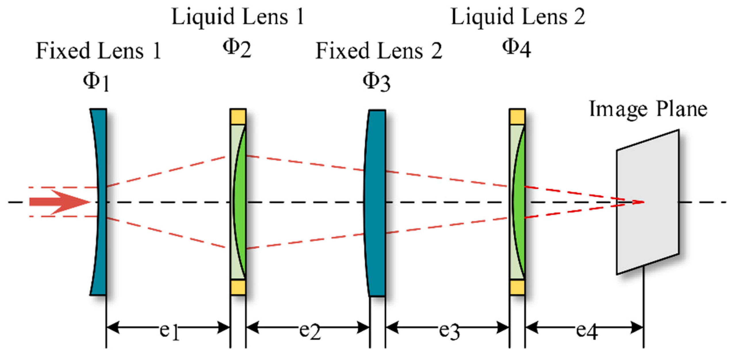
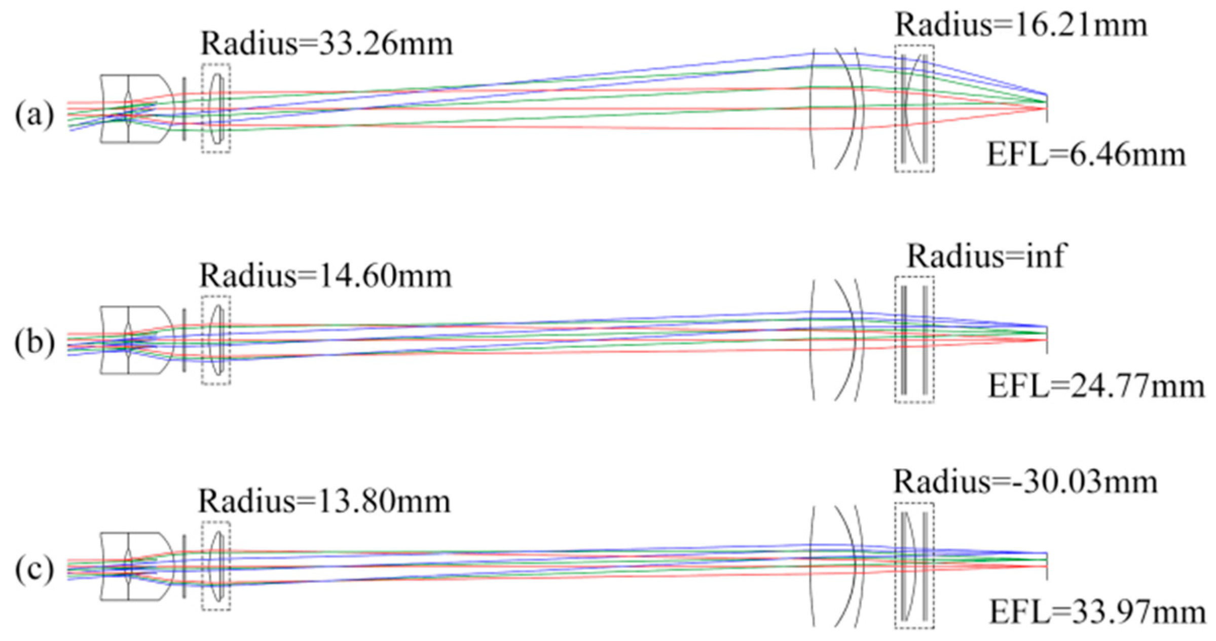
Therefore, the measured EFL range of the zoom system is 6.93 mm to 35.06 mm, the zoom ratio is 5.06:1. When I2 = 5 mA, EFL takes minimum, at this moment Φ2 = 0.0087 mm−1 and Φ4 = 0.0185 mm−1, the FOV is 40°. When I2 = 100 mA, EFL takes maximum, Φ2 = 0.0192 mm−1 and Φ4 = −0.0100 mm−1 at this moment, the FOV is 8°.
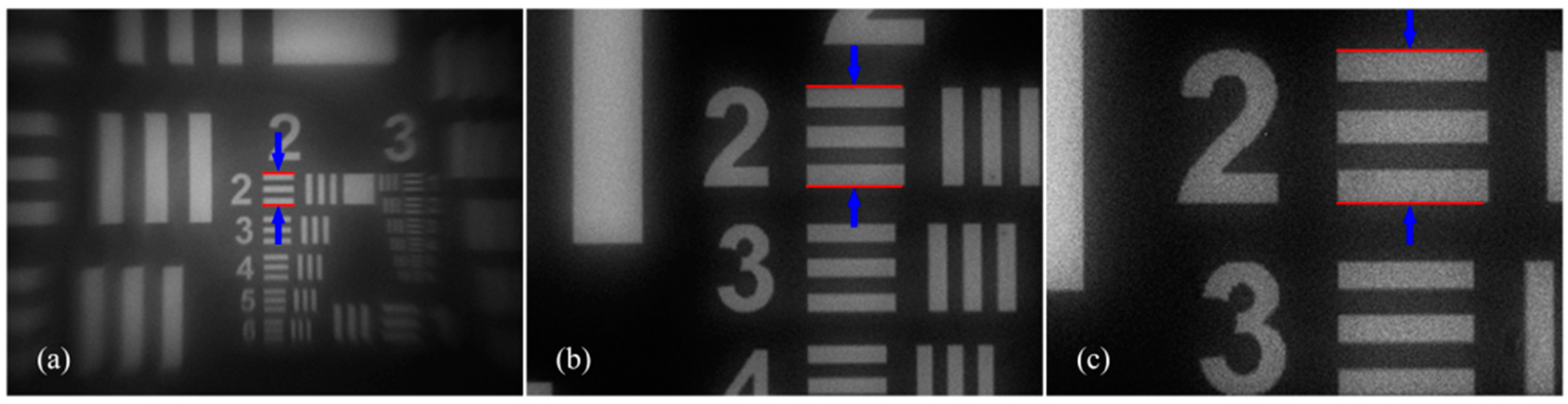
Images captured in different EFL are shown in
Figure 10a–c show the wide end, the middle phase, and the tele end respectively. In wide end, EFL is 6.93 mm, the zoom system has the widest FOV, and there are 18 pixels between two red lines shown in
Figure 10a. In tele end, EFL is 35.06 mm, the zoom system is most detailed, and the number of pixels between two red lines shown in
Figure 10c increases to 91. We can also get the conclusion of a 5.06:1 zoom ratio. A middle phase is presented too, in order to make readers observe the zoom process from wide end to tele end visually.
Figure 10.
Images captured in different EFL. (a) wide end, when I2 = 5 mA, 18 pixels between two red lines; (b) middle phase, when I2 = 60 mA, 59 pixels between two red lines; (c) tele end, when I2 = 100 mA, 91 pixels between two red lines.
Figure 10.
Images captured in different EFL. (a) wide end, when I2 = 5 mA, 18 pixels between two red lines; (b) middle phase, when I2 = 60 mA, 59 pixels between two red lines; (c) tele end, when I2 = 100 mA, 91 pixels between two red lines.
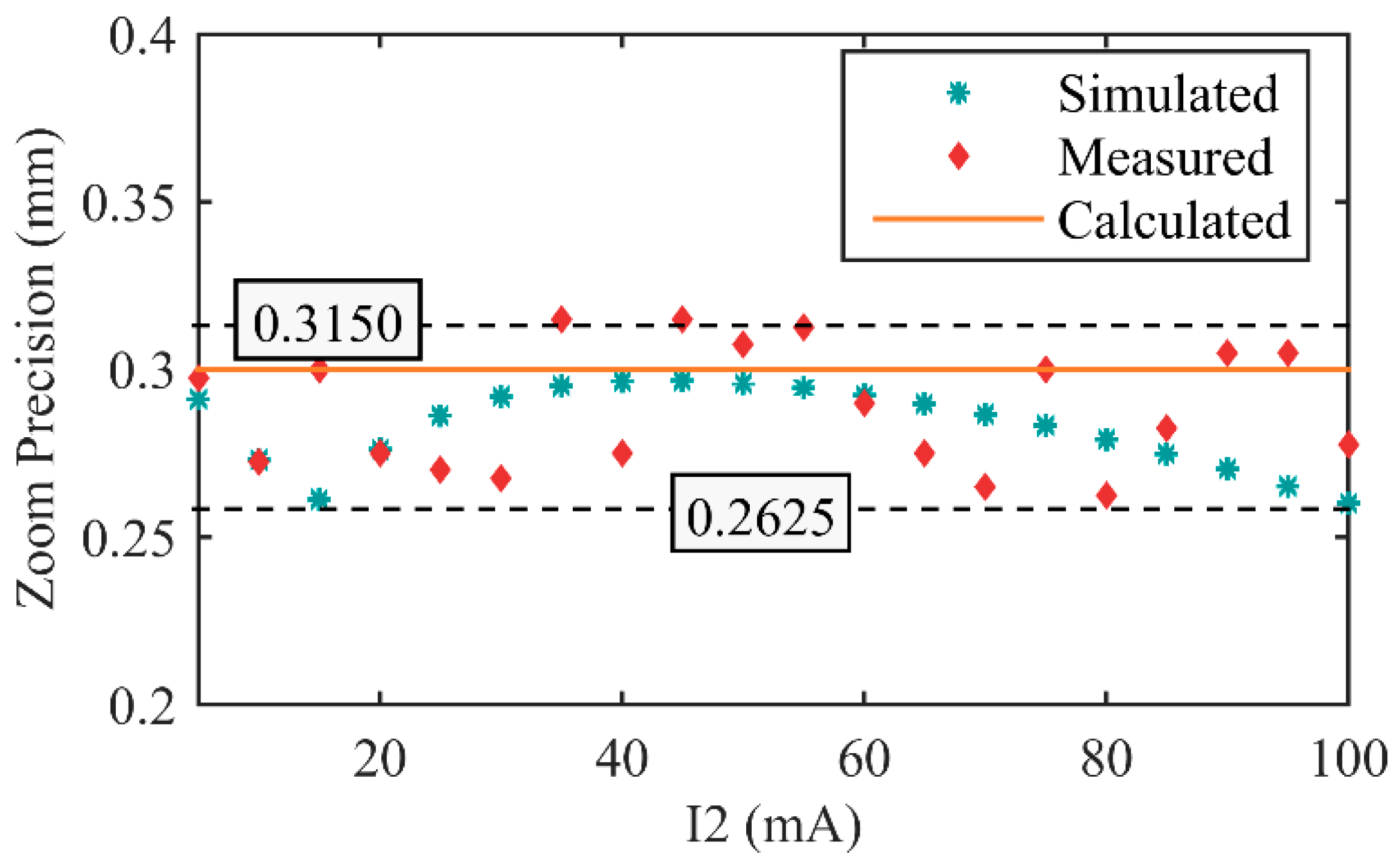
3.5. Zoom Precision Testing
In order to measure the zoom precision of the system, we set I
2 to a value firstly, measured EFL at this moment. Then we adjusted I
2 to increase 1 mA, and measured the variation of EFL. In the above, we had simulated the test process. The simulated results had been shown in
Table 3. The measured results are shown in
Table 6, and diagram of comparison among calculated, simulated, and measured results is shown in
Figure 11.
Table 6.
Measured zoom precision.
Table 6.
Measured zoom precision.
| I2 (mA) | Zoom Precision (mm) | I2 (mA) | Zoom Precision (mm) |
|---|
| 5 | 0.2975 | 55 | 0.3125 |
| 10 | 0.2725 | 60 | 0.2900 |
| 15 | 0.3000 | 65 | 0.2750 |
| 20 | 0.2750 | 70 | 0.2650 |
| 25 | 0.2700 | 75 | 0.3000 |
| 30 | 0.2675 | 80 | 0.2625 |
| 35 | 0.3150 | 85 | 0.2825 |
| 40 | 0.2750 | 90 | 0.3050 |
| 45 | 0.3150 | 95 | 0.3050 |
| 50 | 0.3075 | 100 | 0.2775 |
| Average | 0.2885 | RMS | 0.0181 |
Figure 11.
Zoom precision comparison among calculated, simulated, and measured values.
Figure 11.
Zoom precision comparison among calculated, simulated, and measured values.
Zoom precision of the realized zoom system is approximately uniform in the whole zoom process. The average of measured zoom precision is 0.2885 mm, near to the calculated value 0.3 mm, and all of measured values are in the range of ±0.0265 mm to average zoom precision, RMS of the measured zoom precision is 0.0181 mm. Parameters of the realized lens are consistent with the calculated and simulated values.
Therefore, there are 96 discrete EFL states in the entire zoom range, spaces between adjacent states are approximately uniform to be 0.2885 mm. Because the EFL states are so compact, we can consider the realized system as a continuous zoom system.
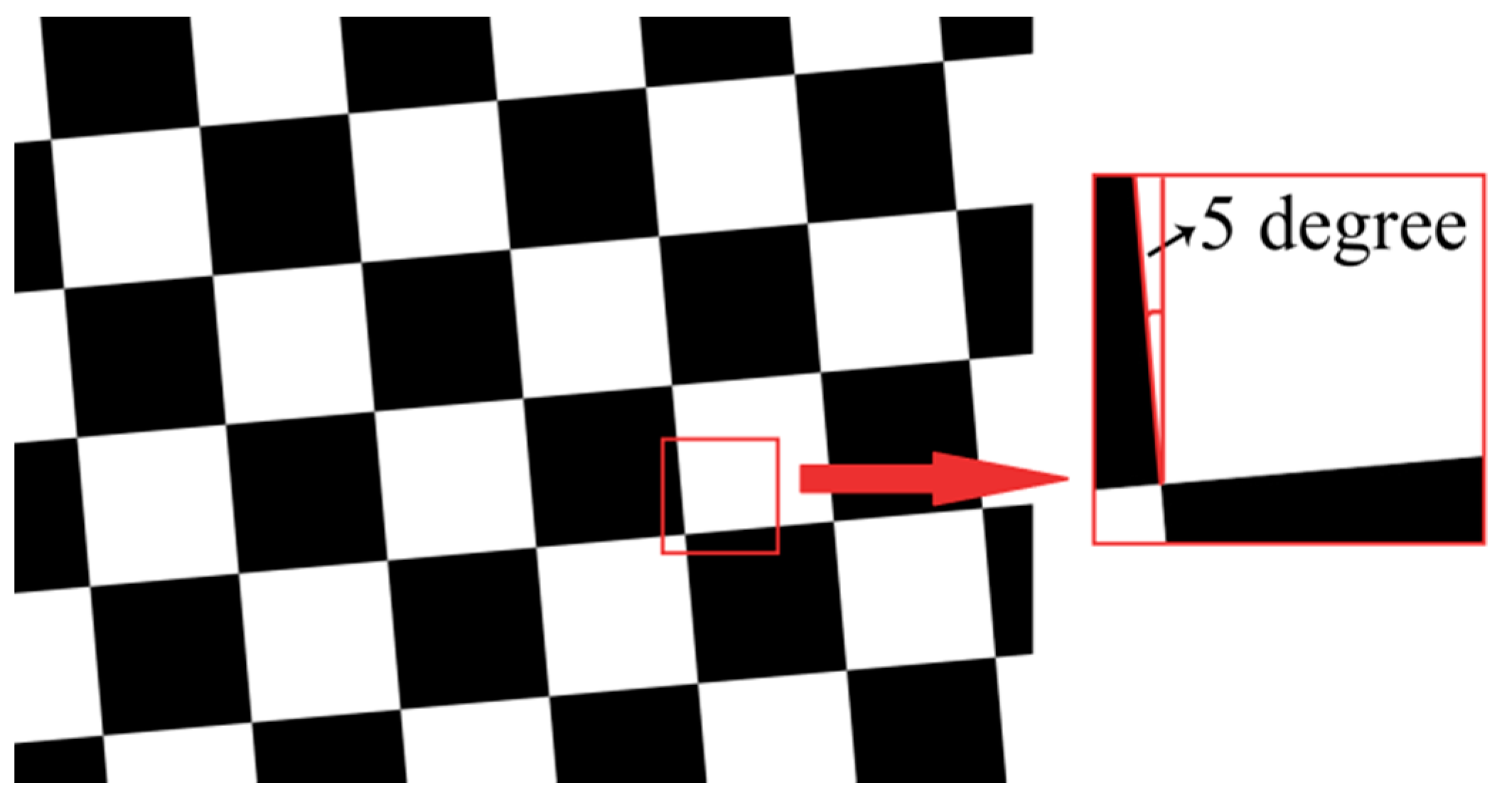
3.6. Imaging Quality Testing
We used MTF to evaluate the imaging quality of the zoom system. The test target used in imaging quality testing is shown in
Figure 12, similar to a black and white chessboard. The tilt of edge was set to 5° according to ISO12233.
Figure 12.
Structure of the target used to test the imaging quality.
Figure 12.
Structure of the target used to test the imaging quality.
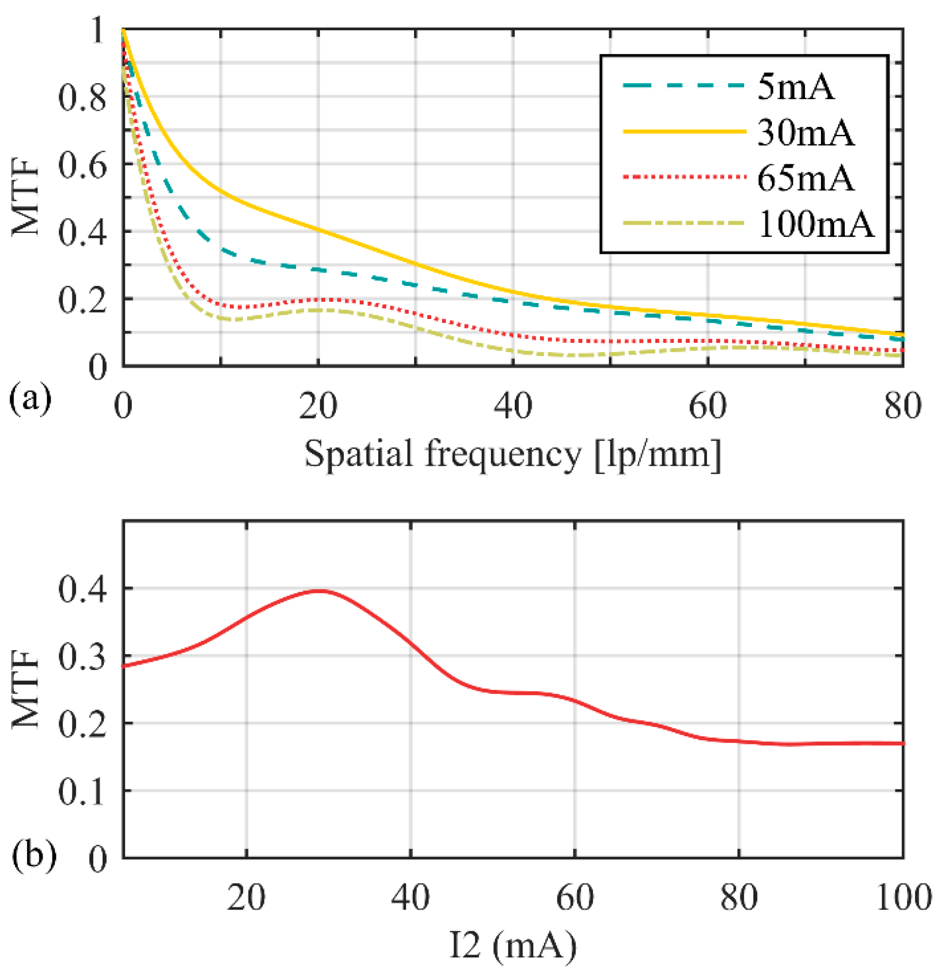
In the test process, we selected a region-of-interest (ROI) that contains a slanted-edge in the beginning, then obtained the Edge Spread Function (ESF) by the use of knife-edge method and got the Line Spread Function (LSF) through the differential of ESF. The MTF could be computed by a Fast Fourier Transform (FFT) of LSF. MTFs were measured when I
2 took different values. The results are shown in
Figure 13a.
Figure 13.
MTF of the zoom system. (a) MTFs were measured when I2 took different values; (b) relationship between MTF and I2 at 20 lp/mm.
Figure 13.
MTF of the zoom system. (a) MTFs were measured when I2 took different values; (b) relationship between MTF and I2 at 20 lp/mm.
At 20 lp/mm, the relationship between MTF and I
2 is shown in
Figure 13b. The zoom system got the highest imaging quality when I
2 = 30 mA, MTF reached 0.40 at 20 lp/mm. When I
2 > 90 mA, MTF reduced to 0.17 at 20 lp/mm.


