
Integrated Fault Diagnosis Algorithm for Motor Sensors of In-Wheel Independent Drive Electric Vehicles

Abstract
:1. Introduction
2. High-Level Fault Diagnosis
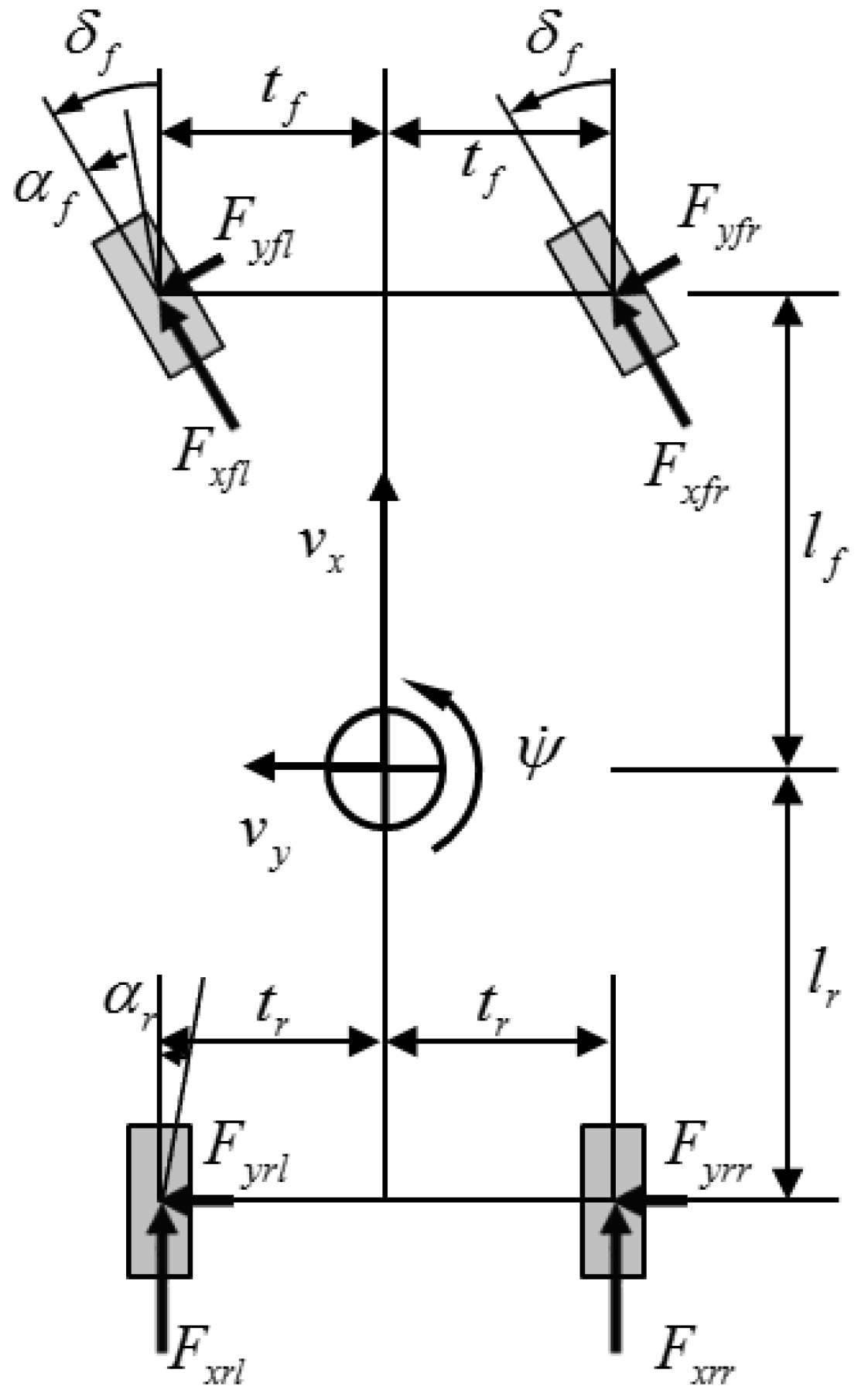
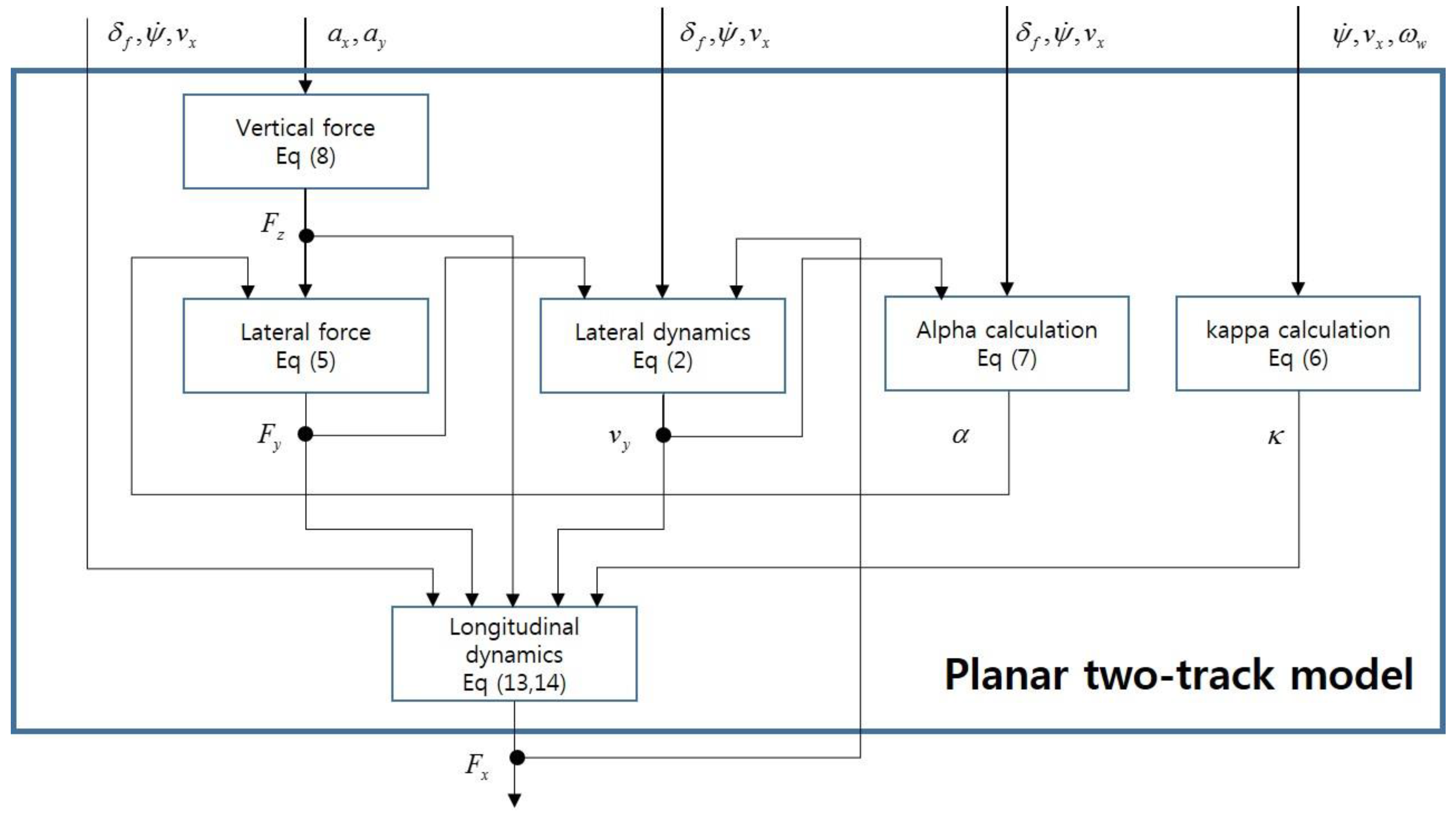
2.1. Planar Two-Track Model
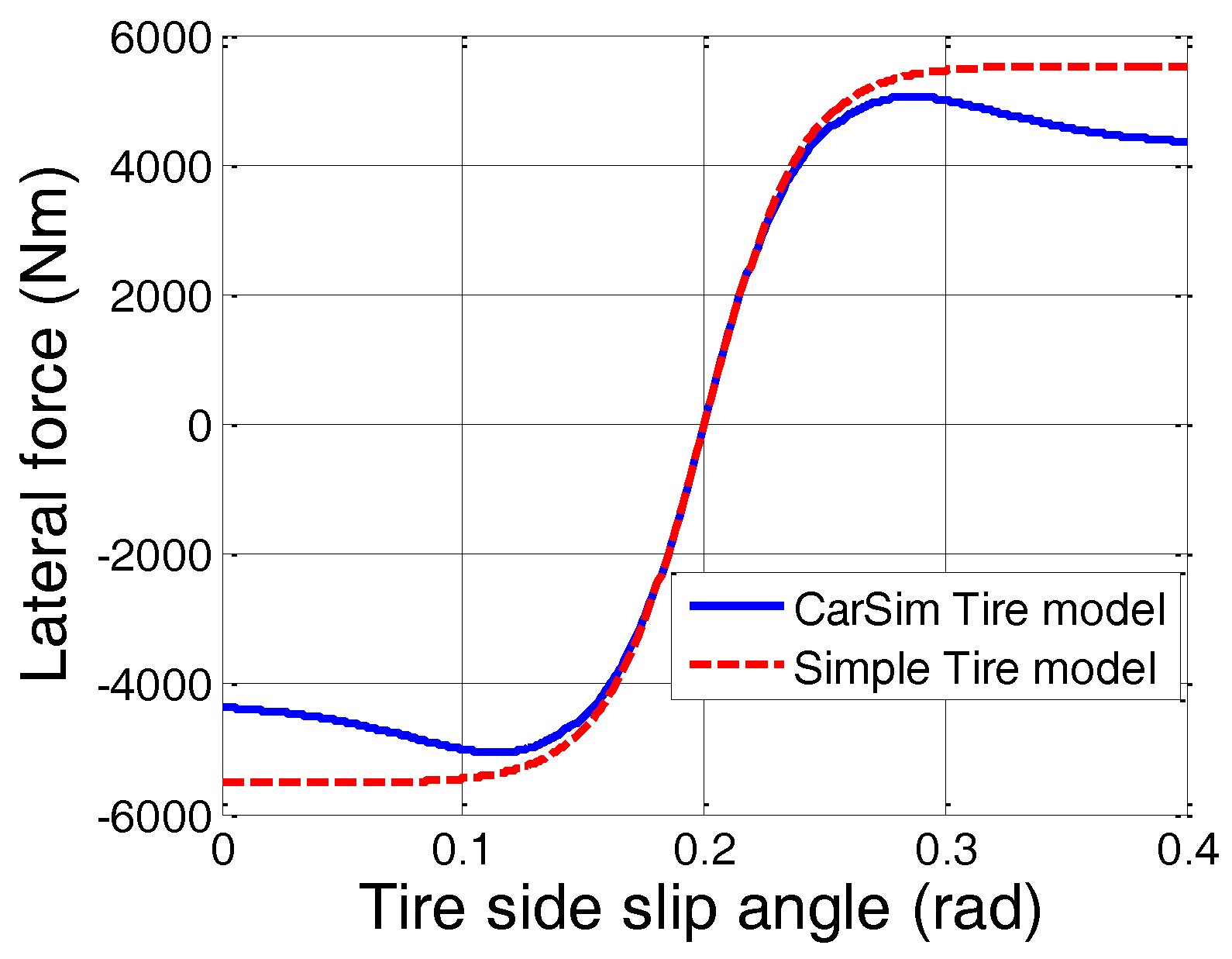
2.2. Non-Linear Simple Tire Model
2.3. Wheel Dynamics
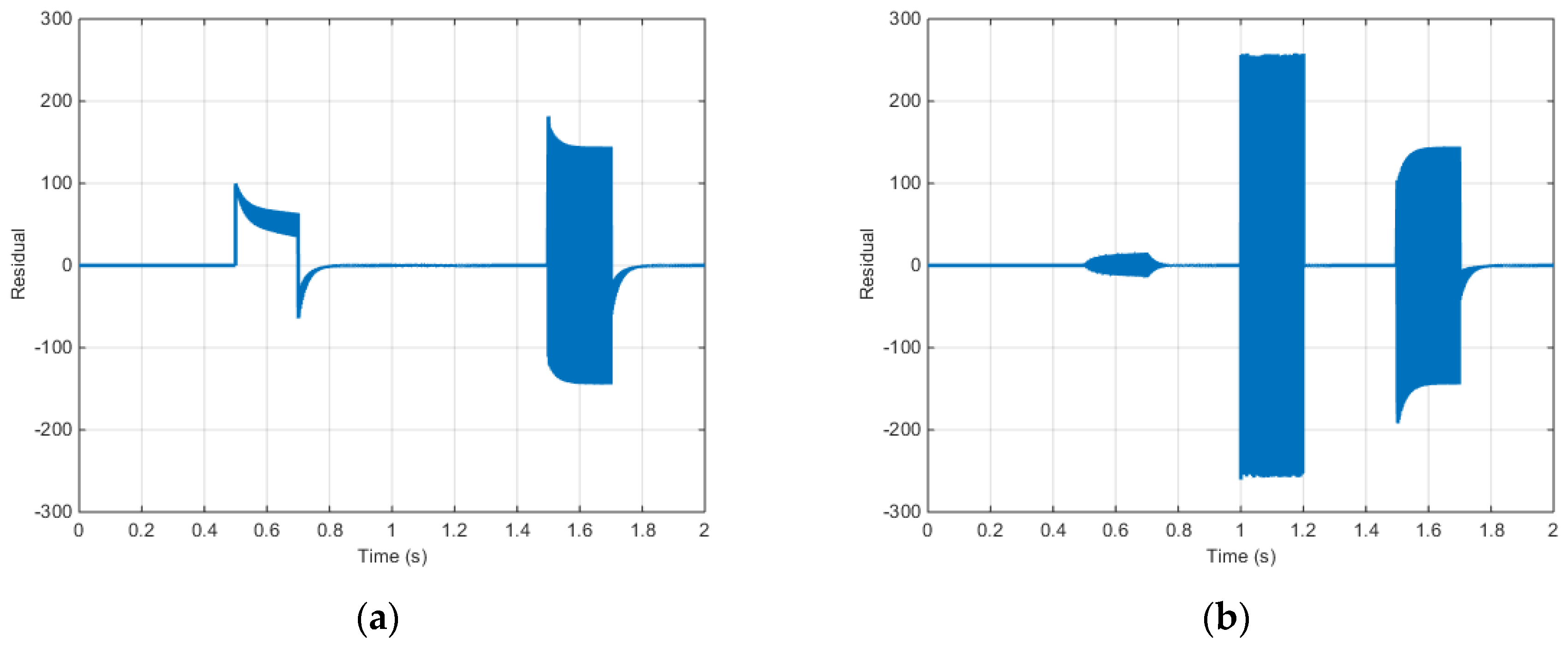
2.4. Residual
2.5. Longitudinal Force Estimation
2.6. Analysis of the Correlation between Each Sensor and the Residual
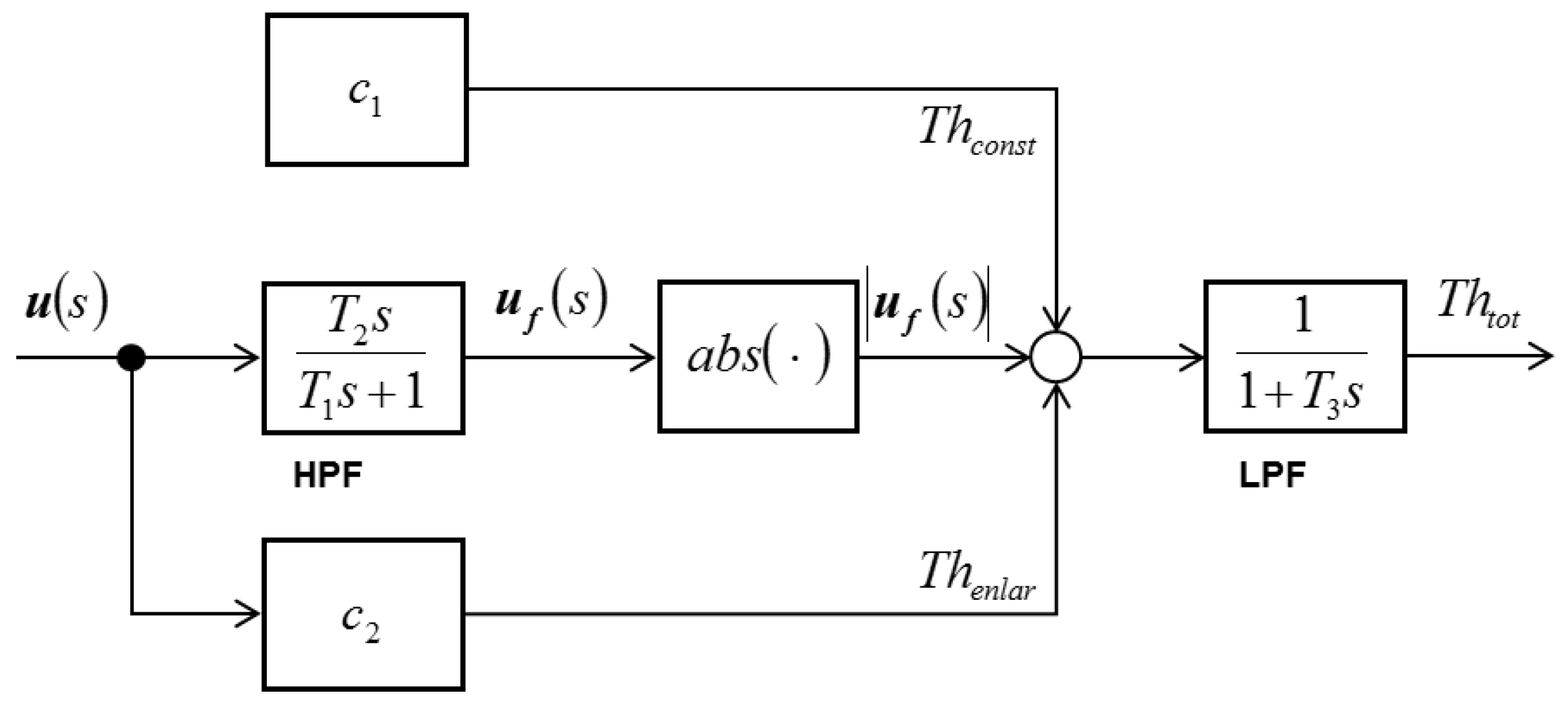
2.7. Adaptive Threshold
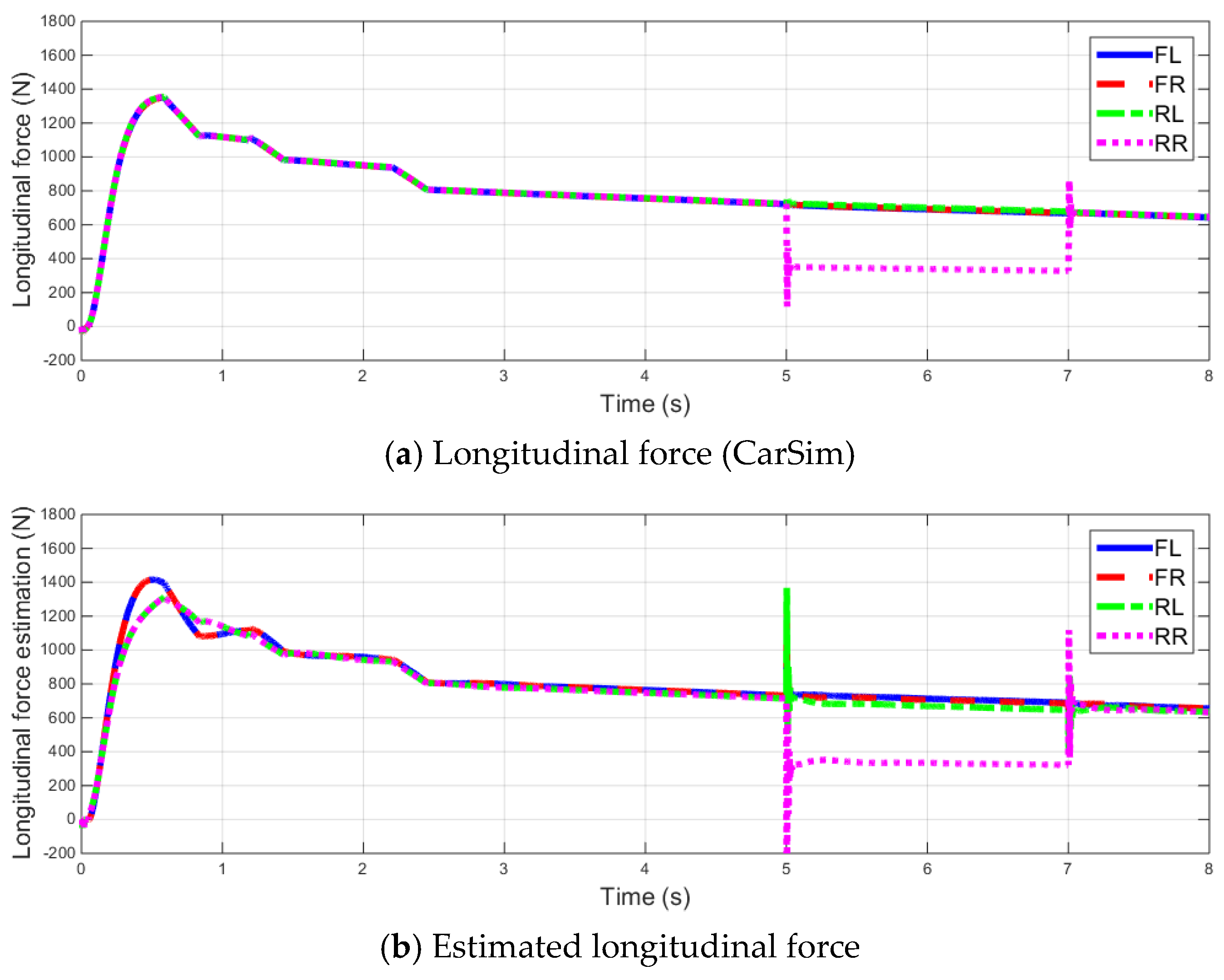
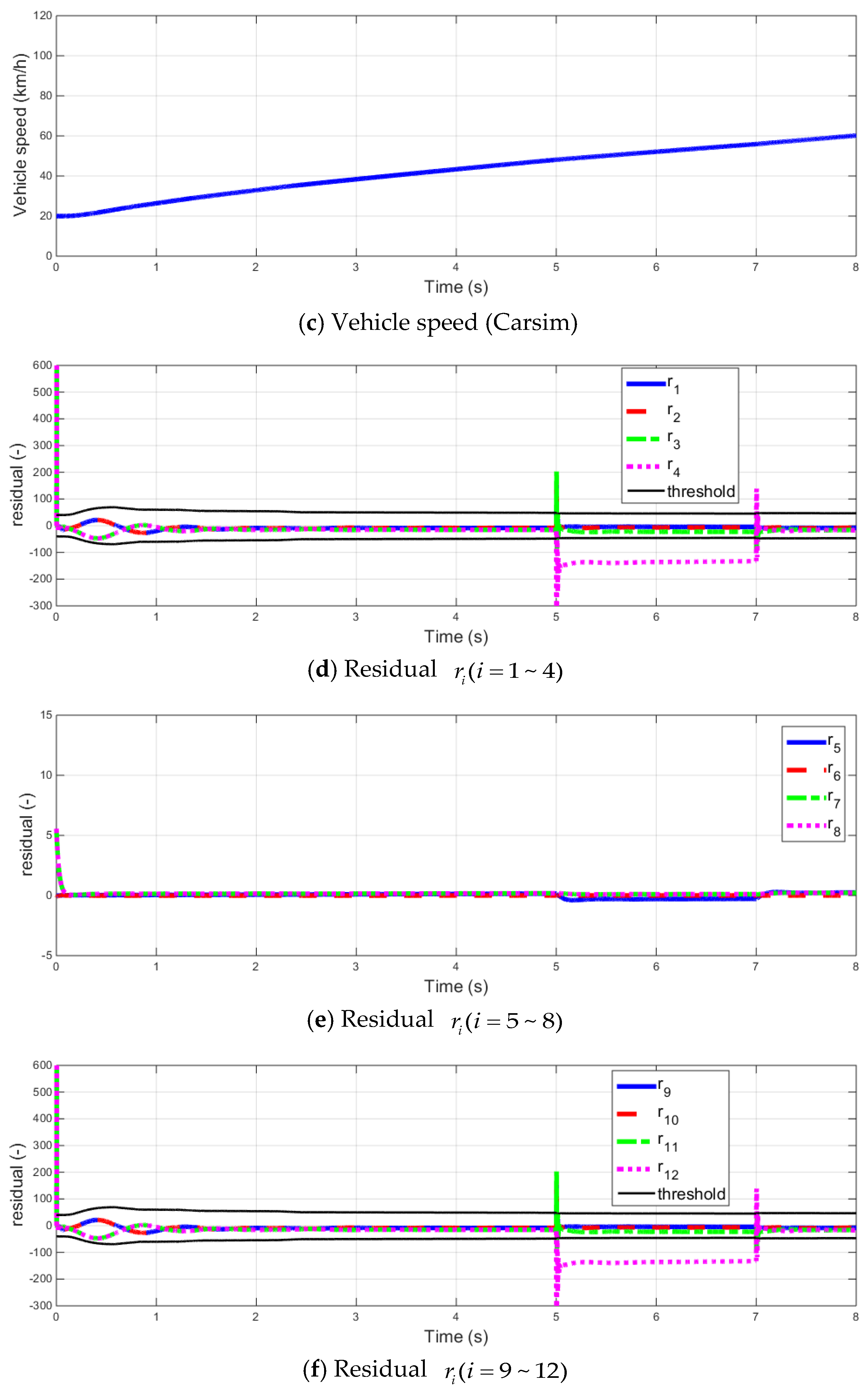
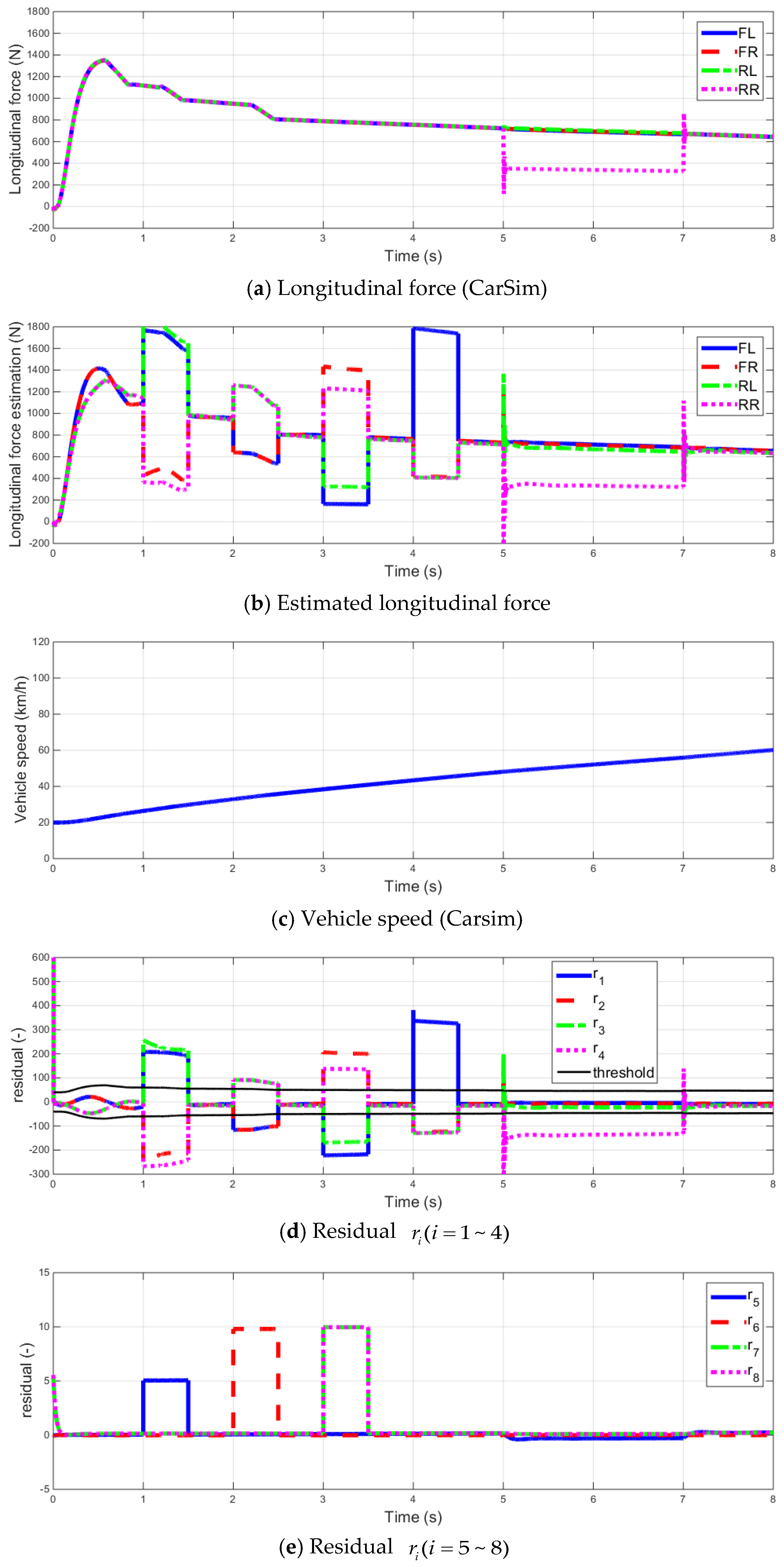
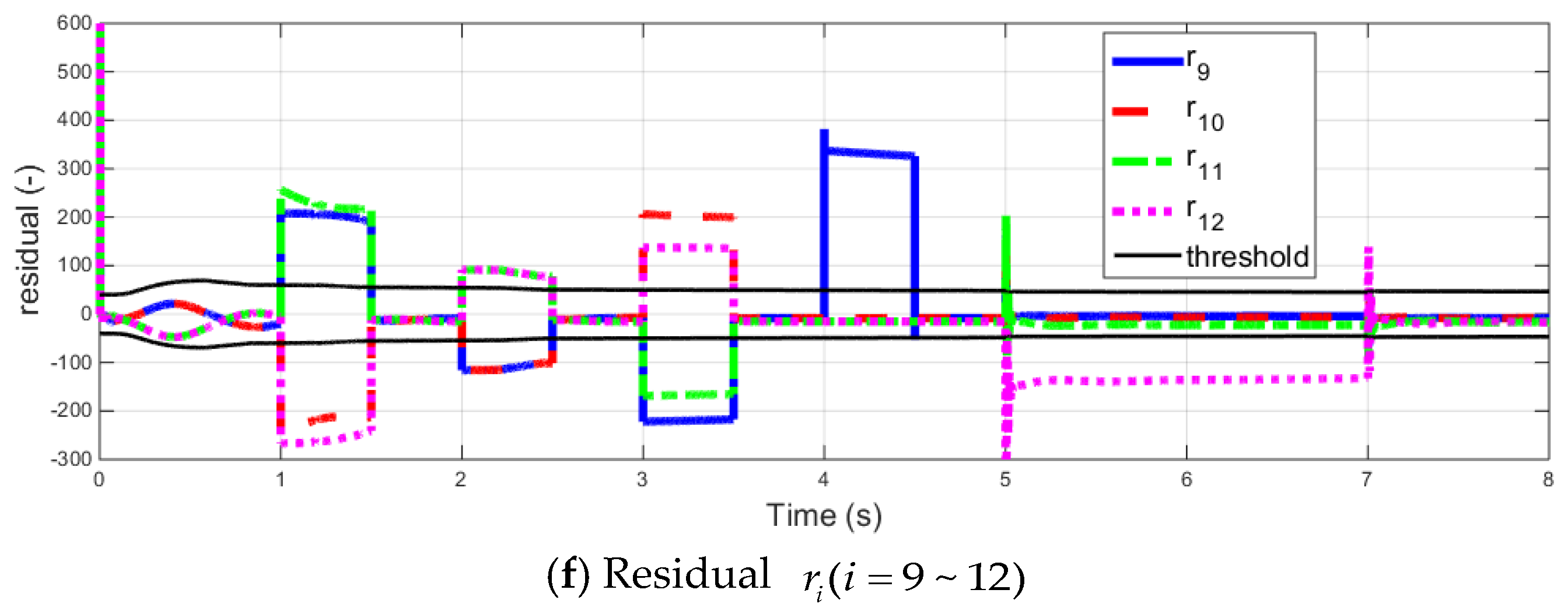
2.8. Simulation Result
3. Low-Level Fault Diagnosis
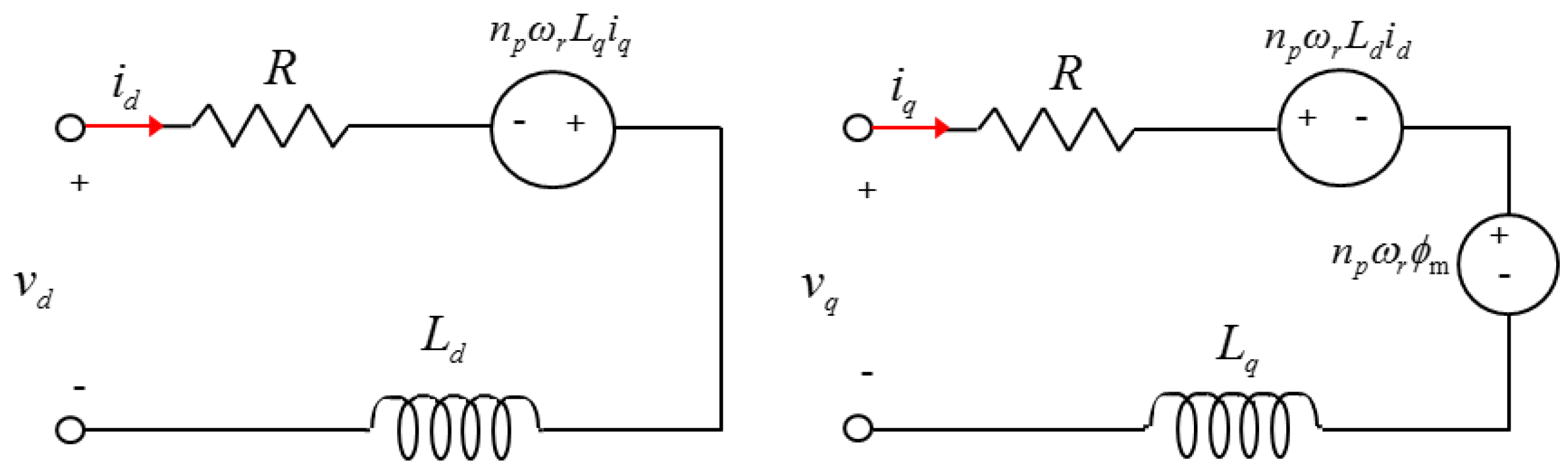
3.1. IPMSM Model
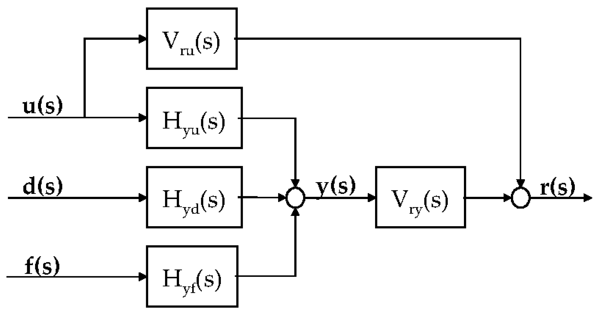
3.2. Current and Position Sensor Fault Diagnosis
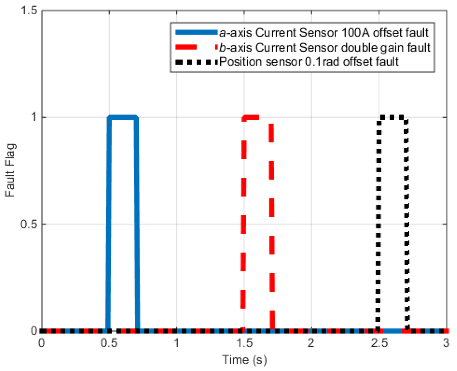
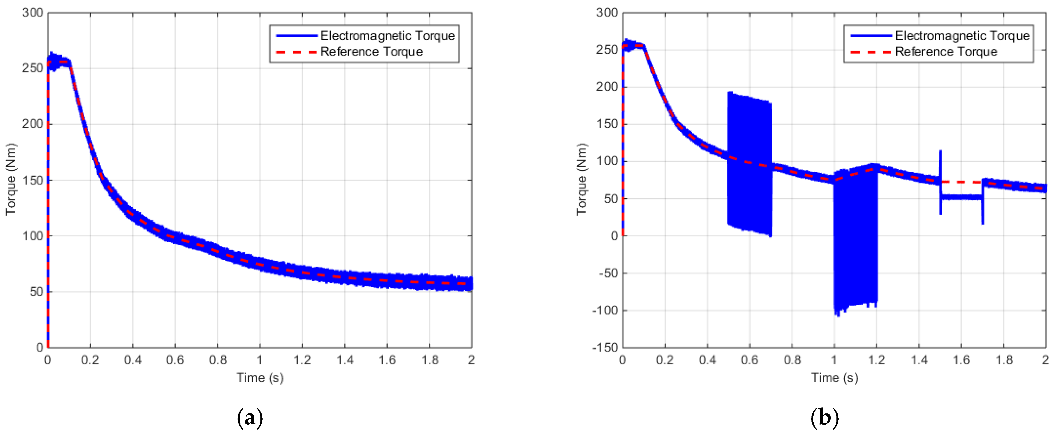
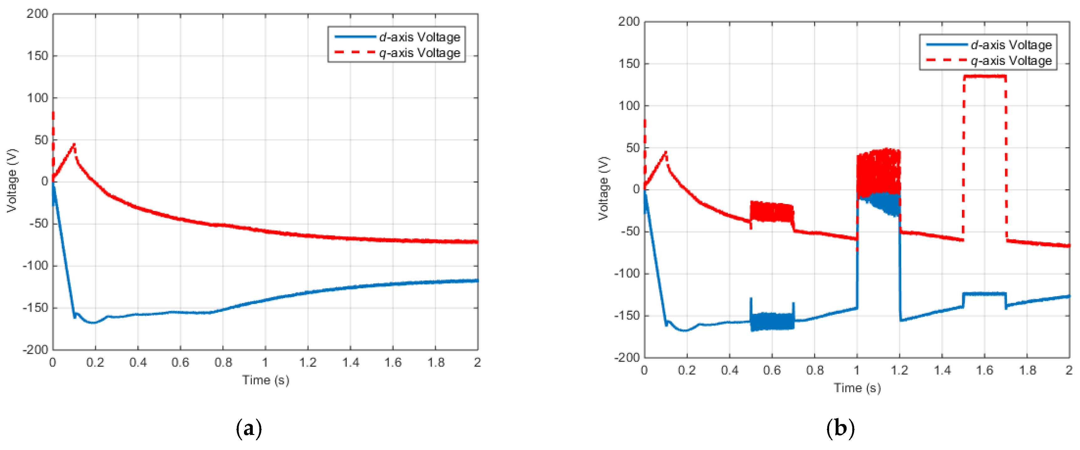
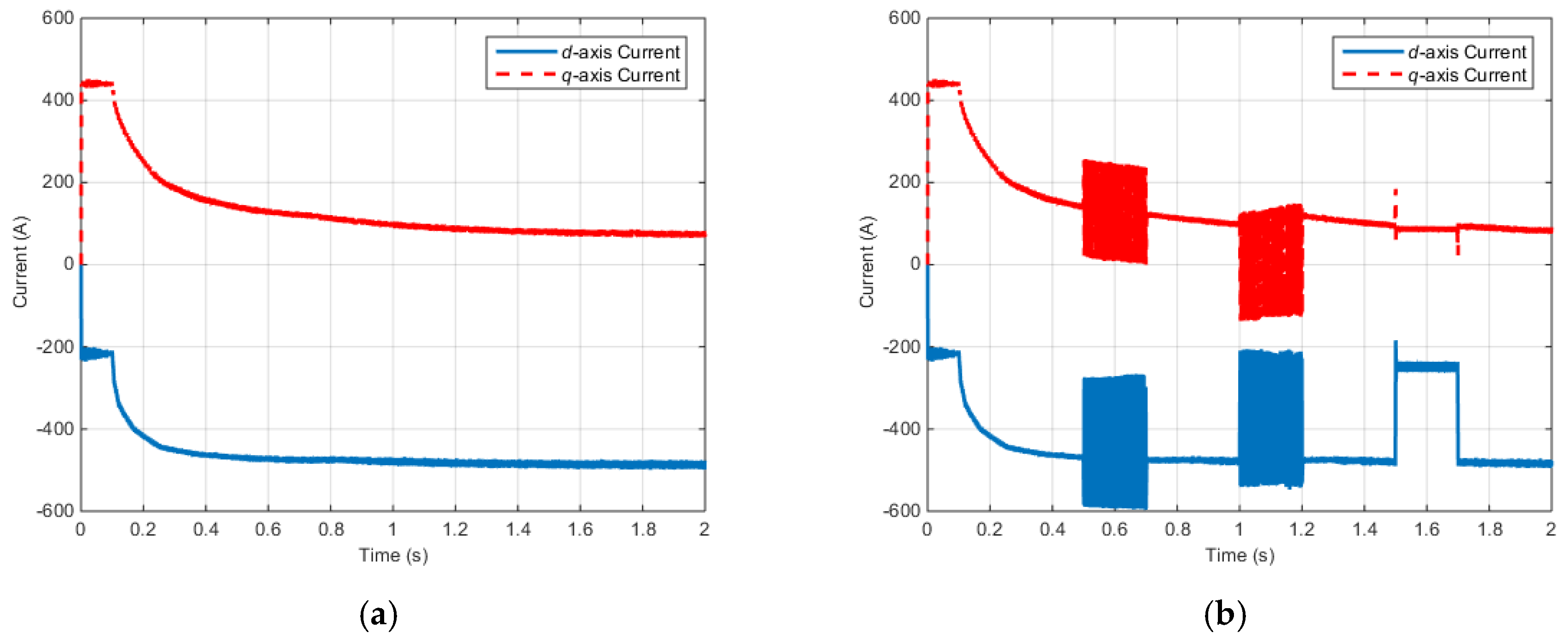
3.3. Simulation Result
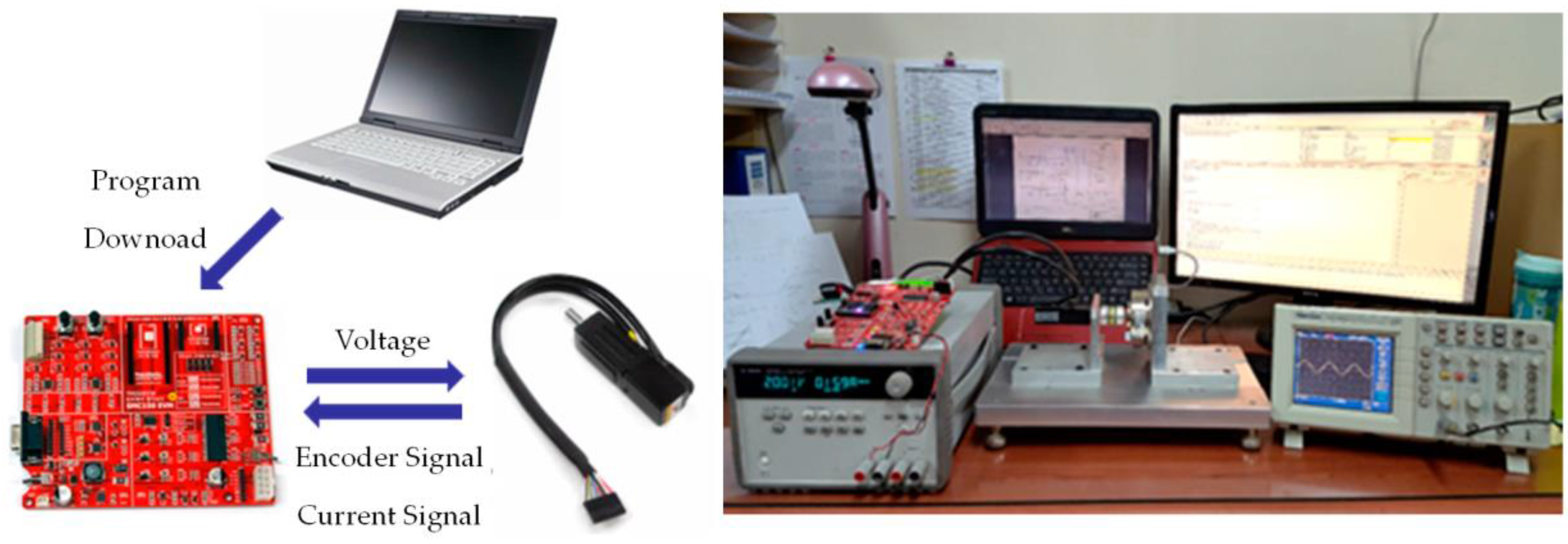
3.4. Experimental Result
4. Integrated Fault-Diagnosis Algorithm
5. Conclusions
Acknowledgments
Author Contributions
Conflicts of Interest
References
- Hori, Y.; Toyoda, Y.; Tsuruoka, Y. Traction control of electric vehicle: Basic experimental results using the test EV UOT Electric March. IEEE Trans. Ind. Appl. 1998, 34, 1131–1138. [Google Scholar] [CrossRef]
- Hori, Y. Future vehicle driven by electricity and control-research on four-wheel-motored UOT Electric March II. IEEE Trans. Ind. Electron. 2004, 51, 954–962. [Google Scholar] [CrossRef]
- Murata, S. Innovation by in-wheel-motor drive unit, Vehicle System Dynamics. Int. J. Veh. Mech. Mobil. 2012, 50, 807–830. [Google Scholar]
- Luo, Y.; Tan, D. Study on the dynamics of the in-wheel motor system. IEEE Trans. Veh. Technol. 2012, 61, 3510–3518. [Google Scholar]
- Chow, E.Y.; Willsky, A.S. Analytical redundancy and the design of robust failure detection systems. IEEE Trans. Autom. Control 1984, 29, 603–614. [Google Scholar] [CrossRef]
- Benbouzid, M.E.H.; Diallo, D.; Zeraoulia, M. Advanced fault-tolerant control of induction-motor drives for EV/HEV traction applications: From conventional to modern and intelligent control techniques. IEEE Trans. Veh. Technol. 2007, 56, 519–528. [Google Scholar] [CrossRef] [Green Version]
- Akin, B.; Ozturk, S.B.; Toliyat, H.; Rayner, M. DSP-based sensorless electric motor fault-diagnosis tools for electric and hybrid electric vehicle powertrain applications. IEEE Trans. Veh. Technol. 2009, 58, 2679–2688. [Google Scholar] [CrossRef]
- Xu, J.; Wang, J.; Li, S.; Cao, B.A. Method to simultaneously detect the current sensor fault and estimate the state of energy for batteries in electric vehicles. Sensors 2016, 16, 1328. [Google Scholar] [CrossRef] [PubMed]
- Huang, G.; Luo, Y.-P.; Zhang, C.-F.; Huang, Y.-S.; Zhao, K.-H. Current sensor fault diagnosis based on a sliding mode observer for PMSM driven systems. Sensors 2015, 15, 11027–11049. [Google Scholar] [CrossRef] [PubMed]
- Huang, G.; Luo, Y.-P.; Zhang, C.-F.; He, J.; Huang, Y.-S. Current sensor fault reconstruction for PMSM Drives. Sensors 2016, 16, 178. [Google Scholar] [CrossRef] [PubMed]
- Lee, B.-H.; Jeon, N.-J.; Lee, H.-C. Current sensor fault detection and isolation of the driving motor for an in-wheel motor drive vehicle. In Proceedings of the 2011 11th International Conference on Control, Automation and Systems (ICCAS 2011), Gyeonggi-do, Korea, 26–29 October 2011; pp. 486–491.
- Kim, Y.-J.; Jeon, N.; Lee, H. Model based fault detection and isolation for driving motors of a ground vehicle. Sens. Transducers 2016, 199, 67–72. [Google Scholar]
- Diallo, D.; Benbouzid, M.E.H.; Makouf, A. A fault-tolerant control architecture for induction motor drives in automotive applications. IEEE Trans. Veh. Technol. 2004, 53, 1847–1855. [Google Scholar] [CrossRef] [Green Version]
- Ifedi, C.J.; Mecrow, B.C.; Brockway, S.T.; Boast, G.S.; Atkinson, G.J.; Kostic-Perovic, D. Fault-tolerant in-wheel motor topologies for high-performance electric vehicles. IEEE Trans. Ind. Appl. 2013, 49, 1249–1257. [Google Scholar] [CrossRef]
- Jeong, Y.-S.; Sul, S.-K.; Schulz, S.E.; Patel, N.R. Fault detection and fault-tolerant control of interior permanent-magnet motor drive system for electric vehicle. IEEE Trans. Ind. Appl. 2005, 41, 46–51. [Google Scholar] [CrossRef]
- Park, B.-G.; Lee, K.-J.; Kim, R.-Y.; Kim, T.-S.; Ryu, J.-S.; Hyun, D. Simple fault diagnosis based on operating characteristic of brushless direct-current motor drives. IEEE Trans. Ind. Electron. 2011, 58, 1586–1593. [Google Scholar] [CrossRef]
- Naidu, M.; Gopalakrishnan, S.; Nehl, T.W. Fault-tolerant permanent magnet motor drive topologies for automotive x-by-wire systems. IEEE Trans. Ind. Appl. 2010, 46, 841–848. [Google Scholar] [CrossRef]
- Parsa, L.; Toliyat, H. Fault-tolerant interior-permanent-magnet machines for hybrid electric vehicle applications. IEEE Trans. Veh. Technol. 2007, 56, 1546–1552. [Google Scholar] [CrossRef]
- Fang, X.; Gertler, J.; Kunwer, M.; Heron, J.; Barkana, T. A double-threshold-testing robust method for fault detection and isolation in dynamic systems. In Proceedings of the American Control Conference, Baltimore, MD, USA, 29 June–1 July 1994; pp. 1979–1983.
- Song, B.; Hedrick, J.K. Fault tolerant nonlinear control with applications to an automated transit bus. Veh. Syst. Dyn. 2005, 43, 331–350. [Google Scholar] [CrossRef]
- Kim, S.; Song, B.; Song, H. Integrated fault detection and diagnosis system for longitudinal control of an autonomous all-terrain vehicle (ATV). Int. J. Automot. Technol. 2009, 10, 505–512. [Google Scholar] [CrossRef]
- Ho, L.M.; Ossmann, D. Fault detection and isolation of vehicle dynamics sensors and actuators for an overactuated X-by-wire vehicle. In Proceedings of the 53rd IEEE Conference on Decision and Control, Los Angeles, CA, USA, 15–17 December 2014.
- Anwar, S.; Chen, L. An analytical redundancy-based fault detection and isolation algorithm for a road-wheel control subsystem in a steer-by-wire system. IEEE Trans. Veh. Technol. 2007, 56, 2859–2869. [Google Scholar] [CrossRef]
- Isermann, R.; Schwarz, R.; Stolzl, S. Fault-tolerant drive-by-wire systems. IEEE Control Syst. 2002, 22, 64–81. [Google Scholar] [CrossRef]
- Jayabalan, R.; Fahimi, B. Monitoring and fault diagnosis of multiconverter systems in hybrid electric vehicles. IEEE Trans. Veh. Technol. 2006, 55, 1475–1484. [Google Scholar] [CrossRef]
- Lia, B.; Dua, H.; Lib, W. Fault-tolerant control of electric vehicles with in-wheel motors using actuator-grouping sliding mode controllers. Mech. Syst. Signal Process. 2016, 72–73, 462–485. [Google Scholar] [CrossRef]
- Zhang, X.; Cocquempot, V. Fault tolerant control for an electric 4WD Vehicle’s path tracking with active fault diagnosis. IFAC Proc. Vol. 2014, 47, 6728–6734. [Google Scholar] [CrossRef]
- Wang, R.; Wang, J. Fault-tolerant control with active fault diagnosis for four-wheel independently-driven electric ground vehicles. IEEE Trans. Veh. Technol. 2011, 60, 4276–4287. [Google Scholar] [CrossRef]
- Djeziri, M.A.; Merzouki, R.; Bouamama, B.O.; Ouladsine, M. Fault diagnosis and fault-tolerant control of an electric vehicle overactuated. IEEE Trans. Veh. Technol. 2013, 62, 986–994. [Google Scholar] [CrossRef]
- Jeon, N.; Park, C.; Lee, H. Fault diagnosis algorithm for driving motor of in-wheel independent drive electric vehicle. In Proceedings of the World Congress on Electrical Engineering and Computer Systems and Science (EECSS 2015), Barcelona, Spain, 13–14 July 2015.
- Jeon, N.; Lee, H. Integrated fault diagnosis algorithm for driving motor of in-wheel independent drive electric vehicle. Trans. Korean Soc. Automot. Eng. 2016, 24, 99–111. [Google Scholar] [CrossRef]
- Zhou, Q.; Ai, Y.; Bao, H. A hybrid vehicle model for advanced cruise control. In Proceedings of the 2003 IEEE International Conference on Intelligent Transportation Systems, Shanghai, China, 12–15 October 2003; pp. 1165–1170.
- Kaiser, G.; Liu, Q.; Hoffmann, C.; Korte, M.; Werner, H. Torque vectoring for an electric vehicle using an LPV drive controller and a torque and slip limiter. In Proceedings of the 2012 IEEE 51st Annual Conference on Decision and Control (CDC), Maui, HI, USA, 10–13 December 2012; pp. 5016–5021.
- Mokhiamar, O.; Abe, M. How the four wheels should share forces in an optimum cooperative chassis control. Control Eng. Pract. 2006, 14, 295–304. [Google Scholar] [CrossRef]
- WIKIPEDIA. Available online: https://en.wikipedia.org/wiki/CarSim (accessed on 8 December 2016).
- CarSim User Reference Manual; Version 4.0.2; Mechanical Simulation Corporation: Ann Arbor, MI, USA, 1997.
- Hac, A.; Nichols, D.; Sygnarowicz, D. Estimation of vehicle roll angle and side slip for crash sensing. In Proceedings of the SAE 2010 World Congress, Detroit, MI, USA, 13–15 April 2010.
- Jazar, R.N. Vehicle Dynamics Theory and Application; Springer: New York, NY, USA, 2014; pp. 609–620. [Google Scholar]
- Tseng, H.E. Dynamic estimation of road bank angle. Veh. Syst. Dyn. 2001, 36, 307–328. [Google Scholar] [CrossRef]
- Isermann, R. Fault-Diagnosis Systems—An Introduction from Fault Detection to Fault Tolerance; Springer: New York, NY, USA, 2006; pp. 107–108. [Google Scholar]
- Soong, W.L.; Ertugrul, N. Field-weakening performance of interior permanent-magnet motors. IEEE Trans. Ind. Appl. 2002, 38, 1251–1258. [Google Scholar] [CrossRef] [Green Version]
- Bianchi, N.; Bolognani, S. Interior PM synchronous motor for high performance applications. In Proceedings of the Power Conversion Conference-Osaka 2002, Osaka, Japan, 2–5 April 2002; pp. 148–153.
- Blanke, M.; Schröder, J. Diagnosis and Fault-Tolerant Control; Springer: Berlin/Heidelberg, Germany, 2006; Volume 2. [Google Scholar]
- Rahman, A.M.; Zhou, P. Analysis of brushless permanent magnet synchronous motors. IEEE Trans. Ind. Electron. 1996, 43, 256–267. [Google Scholar] [CrossRef]


| X | X | X | X | X | X | X | ||||
| X | X | X | X | X | X | X | ||||
| X | X | X | X | X | X | X | ||||
| X | X | X | X | X | X | X |
| X | X | X | X | X | X | X | X | X | |||||
| X | X | X | X | X | X | X | X | X | |||||
| X | X | X | X | X | X | X | X | X | |||||
| X | X | X | X | X | X | X | X | X | |||||
| X | X | ||||||||||||
| X | X | X | |||||||||||
| X | X | X | |||||||||||
| X | X | ||||||||||||
| X | X | X | X | X | X | ||||||||
| X | X | X | X | X | X | ||||||||
| X | X | X | X | X | X | ||||||||
| X | X | X | X | X | X |
| θ | |||
|---|---|---|---|
| X | X | ||
| X | X |
| Parameter Name | Value (Unit) |
|---|---|
| Stator resistance () | 8.296 (mΩ) |
| d-axis stator inductance () | 0.174 (mH) |
| q-axis stator inductance () | 0.293 (mH) |
| Magnet flux linkage () | 71.115 (mV·s) |
| Inertia () | 0.089 (kg·m2) |
| Viscous damping () | 0.005 (Nm·s) |
| Pole pairs () | 4 (-) |
| Parameter Name | Value (Unit) |
|---|---|
| Stator resistance () | 2/3 (Ω) |
| d-axis stator inductance () | 0.51/3 (mH) |
| q-axis stator inductance () | 0.51/3 (mH) |
| Magnet flux linkage () | 1.25 (mV·s) |
| Pole pairs () | 4 (-) |
| Low-Level Fault Diagnosis | High-Level Fault Diagnosis | Fault Isolation | |
|---|---|---|---|
| and | FL Motor | Current sensor | |
| and | Current sensor | ||
| and | Position sensor | ||
| and | FR Motor | Current sensor | |
| and | Current sensor | ||
| and | Position sensor | ||
| and | RL Motor | Current sensor | |
| and | Current sensor | ||
| and | Position sensor | ||
| and | RR Motor | Current sensor | |
| and | Current sensor | ||
| and | Position sensor | ||
| and | Intolerable and not isolatable | ||
| or | Tolerable and isolatable | ||
© 2016 by the authors; licensee MDPI, Basel, Switzerland. This article is an open access article distributed under the terms and conditions of the Creative Commons Attribution (CC-BY) license (http://creativecommons.org/licenses/by/4.0/).
Share and Cite
Jeon, N.; Lee, H. Integrated Fault Diagnosis Algorithm for Motor Sensors of In-Wheel Independent Drive Electric Vehicles. Sensors 2016, 16, 2106. https://doi.org/10.3390/s16122106
Jeon N, Lee H. Integrated Fault Diagnosis Algorithm for Motor Sensors of In-Wheel Independent Drive Electric Vehicles. Sensors. 2016; 16(12):2106. https://doi.org/10.3390/s16122106
Chicago/Turabian StyleJeon, Namju, and Hyeongcheol Lee. 2016. "Integrated Fault Diagnosis Algorithm for Motor Sensors of In-Wheel Independent Drive Electric Vehicles" Sensors 16, no. 12: 2106. https://doi.org/10.3390/s16122106
APA StyleJeon, N., & Lee, H. (2016). Integrated Fault Diagnosis Algorithm for Motor Sensors of In-Wheel Independent Drive Electric Vehicles. Sensors, 16(12), 2106. https://doi.org/10.3390/s16122106