5.1. Interpretation Performance of the Far-Field Model
To test the performance of far-field scene interpretation, the test data are collected using the same sensor platform as in [
23]. The sensor platform is mounted on a human body, and the image frames are recorded while walking along various pedestrian paths.
The example images collected from the three test scenes are shown in
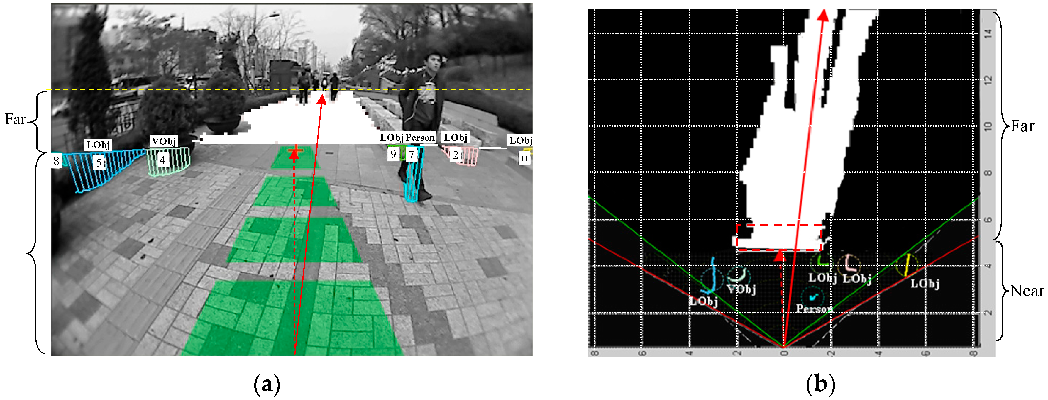
Figure 19. The complexity of the road condition increases from scene ① to scene ③. The image areas between the two dashed lines correspond to the far-field area that needs to be interpreted. In the experiment, the image frames are sampled every three seconds to allow enough variance in the evaluation set. Finally, one hundred image frames from each test scene are selected for the experiment. The ground and object areas in these evaluation image frames are manually labelled as ground truth data.
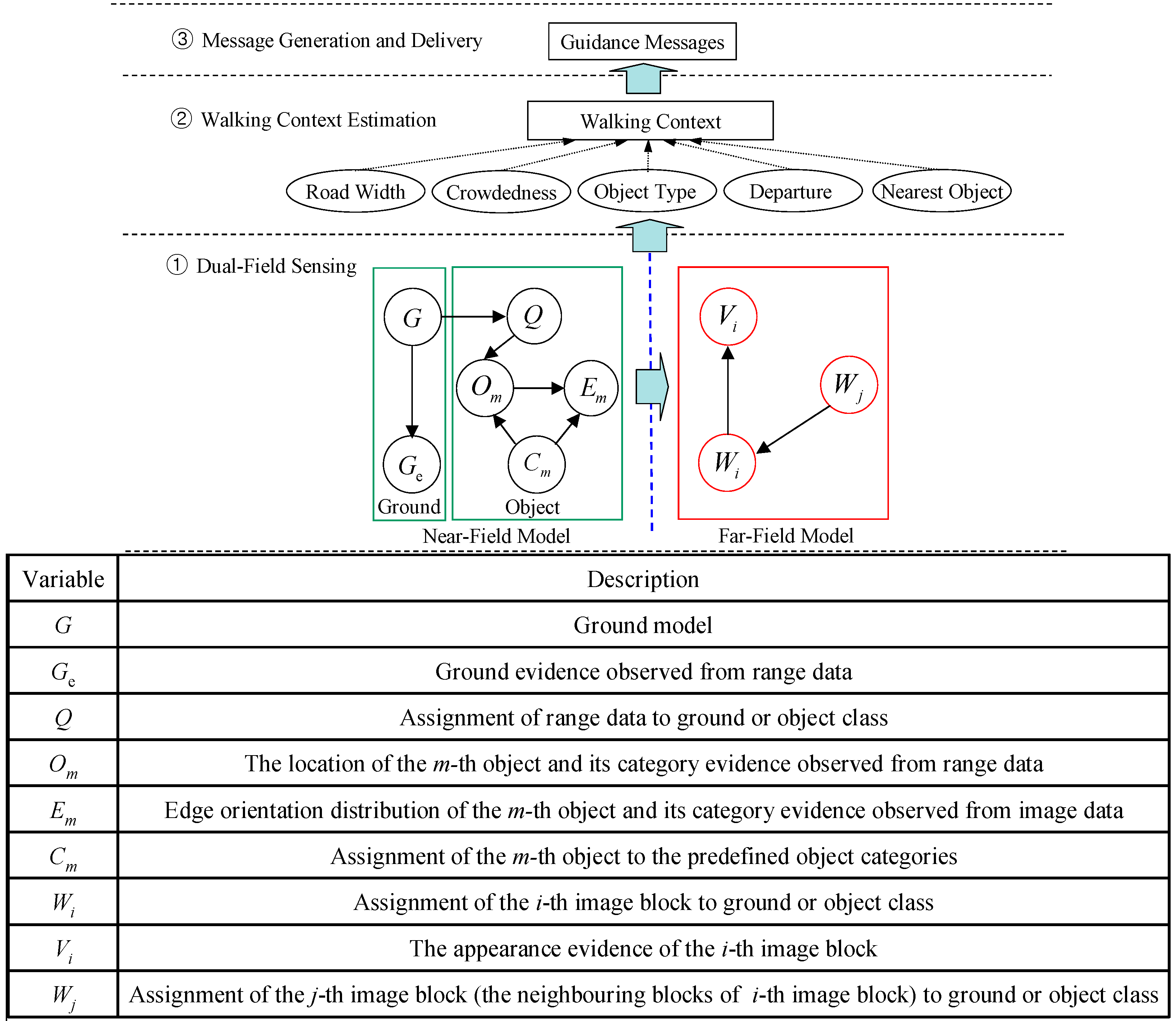
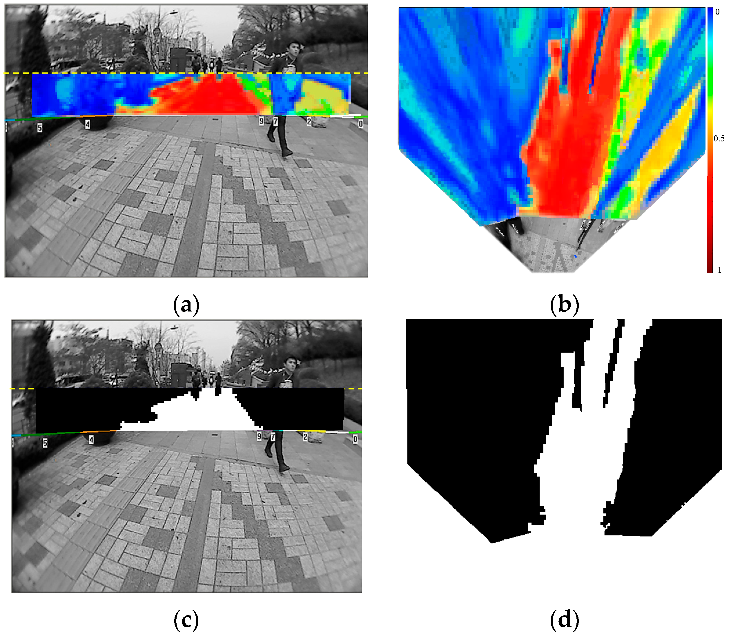
During the experiment, the appearance and spatial prototypes are built on-line using the near-field interpreted data in the preceding frames of each evaluation image frame. Next, the far-field image data in each evaluation image frame are interpreted using the built prototypes based on the far-field graphical model. As a result, a far-field ground probability map P (
Wi = g,
Vi,
Wj) is obtained for each evaluation image frame. The decision rule ‘P (
Wi = g,
Vi,
Wj) > U’ is used to interpret an image block as ground. For each specific value of (U), the interpreted ground areas in the evaluation image frames are compared with the ground truth data to calculate the average true positive (TP) rate and false positive (FP) rate. After the average TP and FP rates are calculated at a specific decision threshold (U), the decision threshold (U) is varied to get other combinations of TP and FP rates. Finally, the receiver operating characteristic (ROC) curves of each test scene are obtained, as shown in
Figure 20.
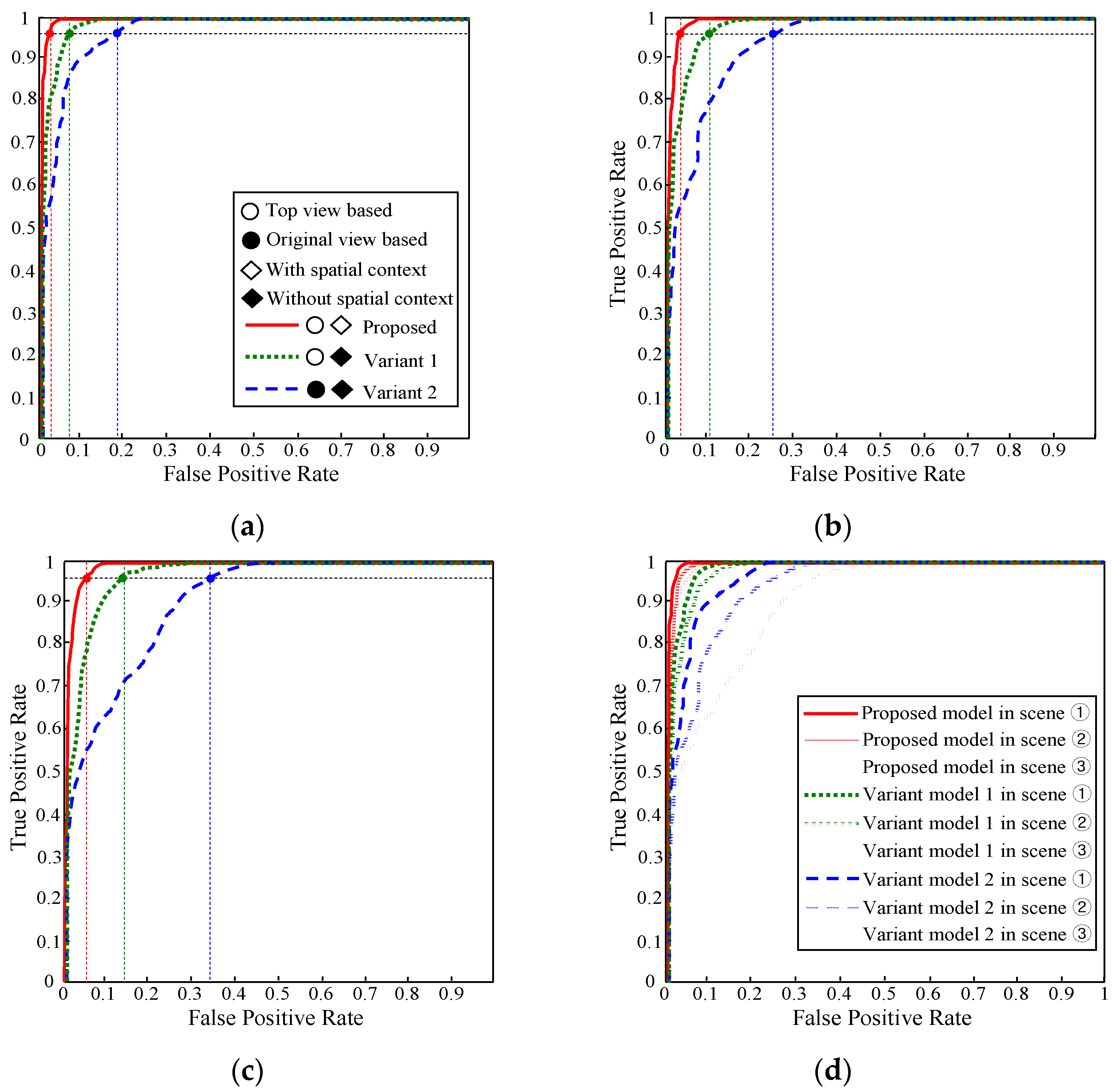
The ROC curves in
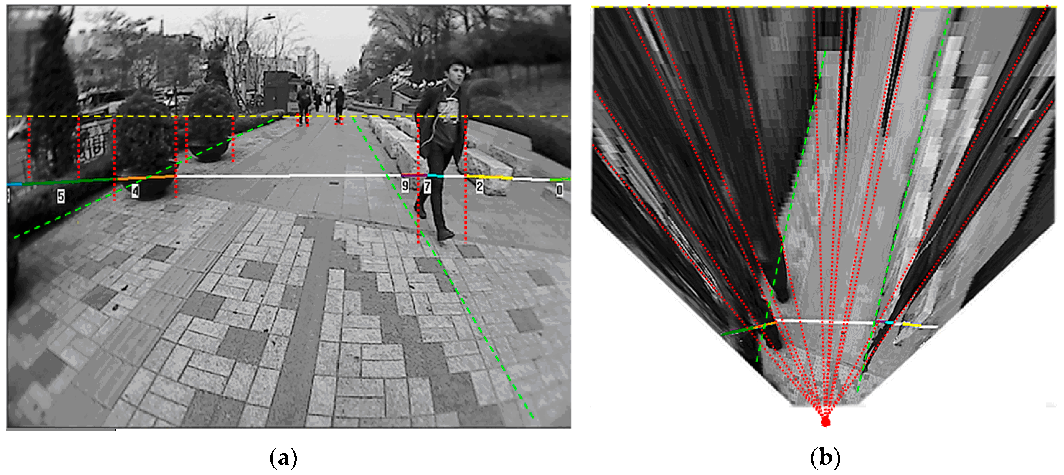
Figure 20 show the interpretation performance of three far-field models. The red solid curve represents the proposed far-field model that uses a top view-based appearance interpretation and spatial context propagation. The green dotted curve shows a variant model 1 that uses a top view-based appearance interpretation without spatial context propagation. The blue dashed curve corresponds to a variant model 2 that uses a perspective view-based appearance interpretation without spatial context propagation. Based on the ROC curves, the variant model 2 performs the worst. This is mainly due to the trouble caused by perspective distortion of the prototype building and matching of local texture descriptors. The variant model 1 that uses top view-based prototype building and matching has a remarkable performance gain over the variant model 2. The effect of the spatial context propagation is verified by comparing the red solid curve to the green dotted curve. The extra performance gain of the proposed model shows that the special context helps to remove many spatially inconsistent errors caused by local appearance descriptor matching.
The proposed far-field model also shows stable performance under different road conditions. As shown in
Figure 20a–c, the performance can be evaluated using the variation of the FP rate of the three models at a fixed TP rate of 96% across the three test scenes. The FP rate of the proposed model only degrades from 3.1% in test scene ① to 5.6% in test scene ③. However, the FP rate of the variant model 1 increases from 8.2% to 14.7%, and the FP rate of the variant model 2 increases from 18.8% to 34.5%. The performance variation across the three test scenes can be more easily observed in
Figure 20d, where the ROC curves of the three test scenes are drawn onto the same graph. It shows that the proposed model maintains a low FP rate consistently at a high TP rate under different road conditions.
Figure 21 shows the far-field interpretation accuracy with respect to the time domain. In this experiment, 200 image frames from the test scene ③ are sampled consecutively at a frequency of 0.5 HZ. For each sampled frame, the accuracy is calculated as the number of correctly interpreted ground and object pixels divided by the number of all pixels in the far-field domain. The red curve shows the accuracy of a far-field model that uses the proposed on-line prototype (appearance + spatial context) building, and the blue curve corresponds to a far-field model that uses an offline prototype built from the initial frames of test scene ③.
It can be observed from
Figure 21 that the accuracy of the off-line model deteriorates significantly from around 44 frames, while the accuracy of the on-line model remains relatively high throughout the experiment. The reason for the different behaviours in interpretation accuracy is due to the change in road appearance. In the first 40 frames, there is not much change in road appearance from the first few initial frames; therefore, the accuracy of the on-line and off-line model is similar. However, when there is significant change in road appearance from around frame 44, the off-line model fails to adapt to the changing environment, which leads to degradation in interpretation accuracy. In contrast, the on-line model achieves a steady accuracy above 90% despite the change in road appearance, showing its capability of adapting to the road environment.
Regarding the proposed far-field interpretation model, its interpretation performance is related to several important model parameters. Several experiments are conducted to determine the effects of these model parameters, and the results are shown in
Figure 22.
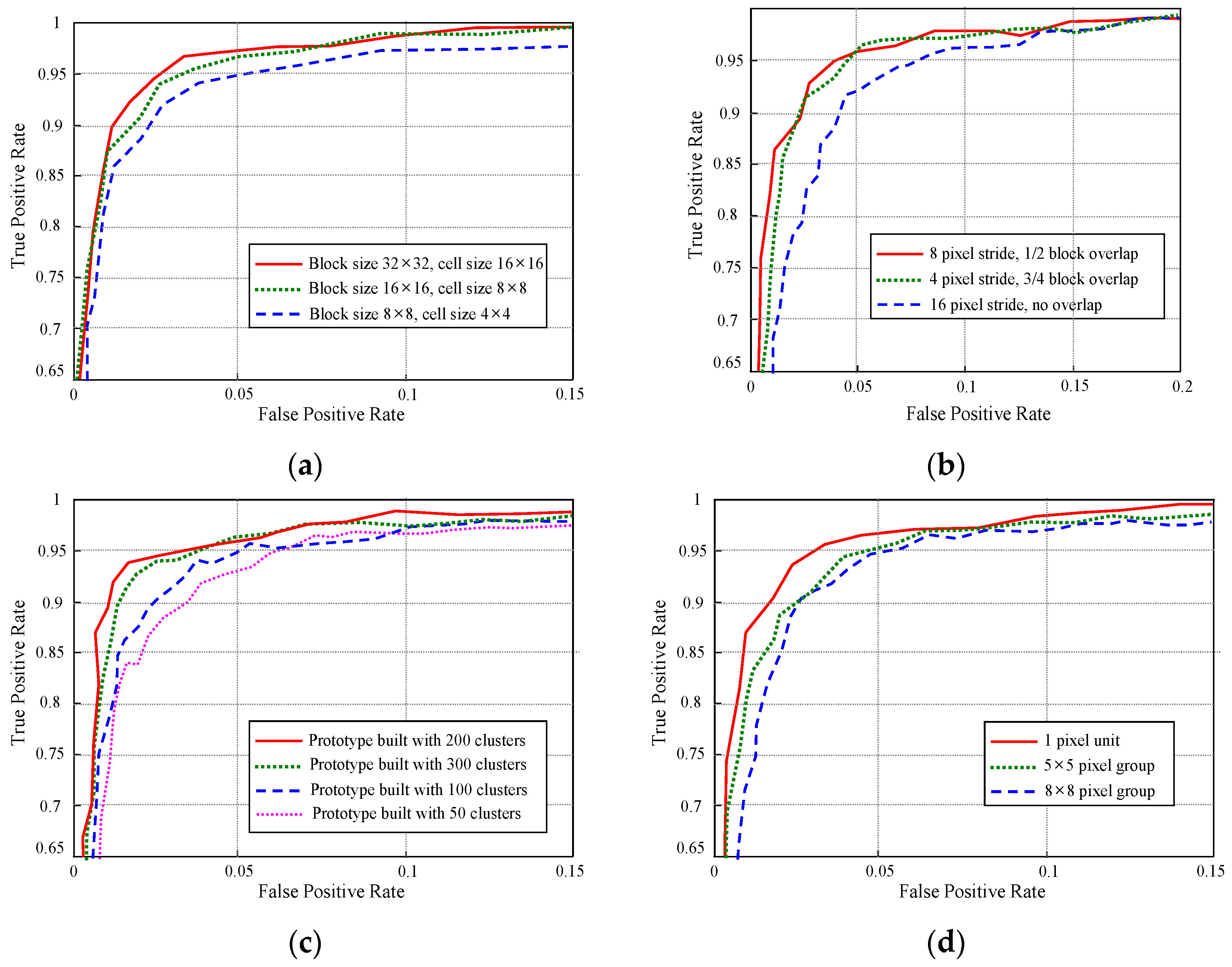
The experiment result as shown in
Figure 22a measures the far-field model performance with respect to the image block size, which is an important parameter that influences the interpretation performance of the appearance prototype. In this experiment, the sample images from test scene ② are used to run the far-field model with all other parameters fixed, only varying the image block size. It turns out that small block size as 8 × 8 is not large enough to contain distinct appearance features inside the block area. Therefore, the interpretation performance of 8 × 8 block is lower than that of 16 × 16 and 32 × 32. Although 32 × 32 block shows a little better performance compared with 16 × 16 block, 16×16 block size is adopted in our far-field model to achieve a balance between interpretation accuracy and interpretation resolution.
Figure 22b shows an experiment on the stride length during the appearance prototype matching. This experiment is carried out using sample images from test scene ③. The image block size is set to 16 × 16 in the experiment. The experimental result demonstrates a very close performance for models that use 4-pixel and 8-pixel stride. Considering the moving efficiency during prototype matching, the 8-pixel stride length is used in the far-field model.
Another parameter that related to the far-field model performance is the size of the appearance prototype. The sample images from test scene ① are used to conduct this experiment on the prototype size. As shown in
Figure 22c, if the prototype size is too small, it may not be able to represent the general appearance pattern comprehensively. Therefore, the model that uses a 50 cluster prototype behaves the worst in interpretation performance. However, if the prototype size is too large, the on-line update rate of some outdated clusters in the prototype will be decreased. This might increase the risk of making interpretation errors that are caused by matching with some outdated appearance patterns in the prototype. Based on the results of the experiment, a medium size of 150 clusters is generally used for the appearance prototype building. The performance of far-field model is also related to the size of pixel group that is used in building spatial context prototype. The experiment result in
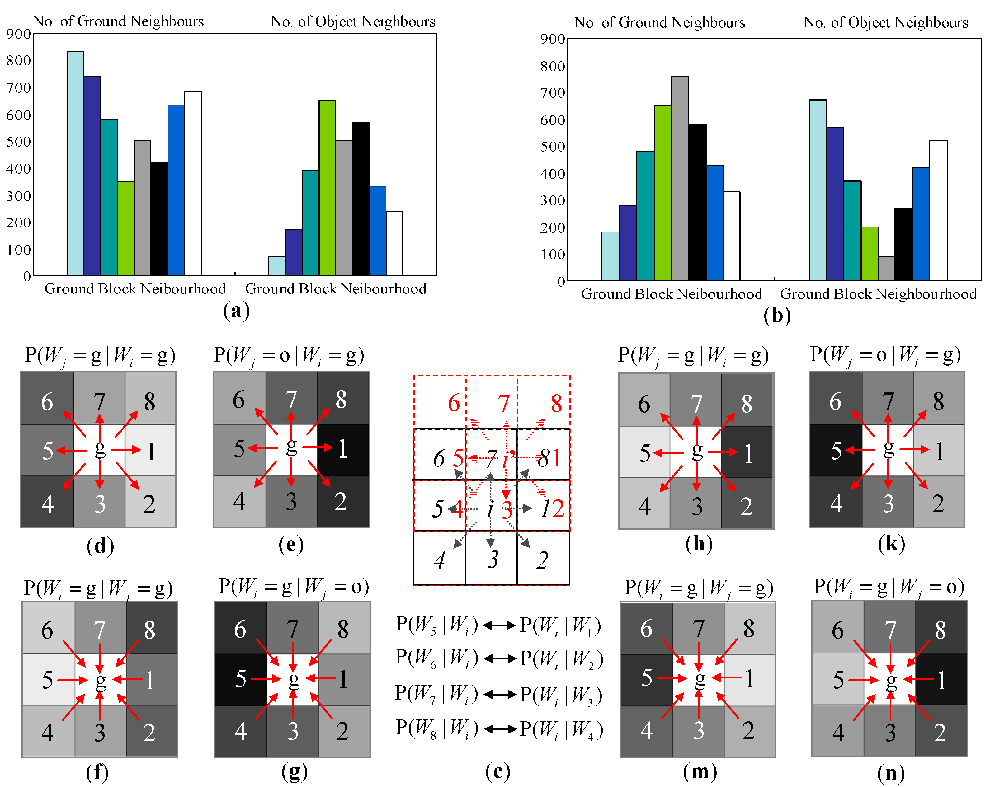
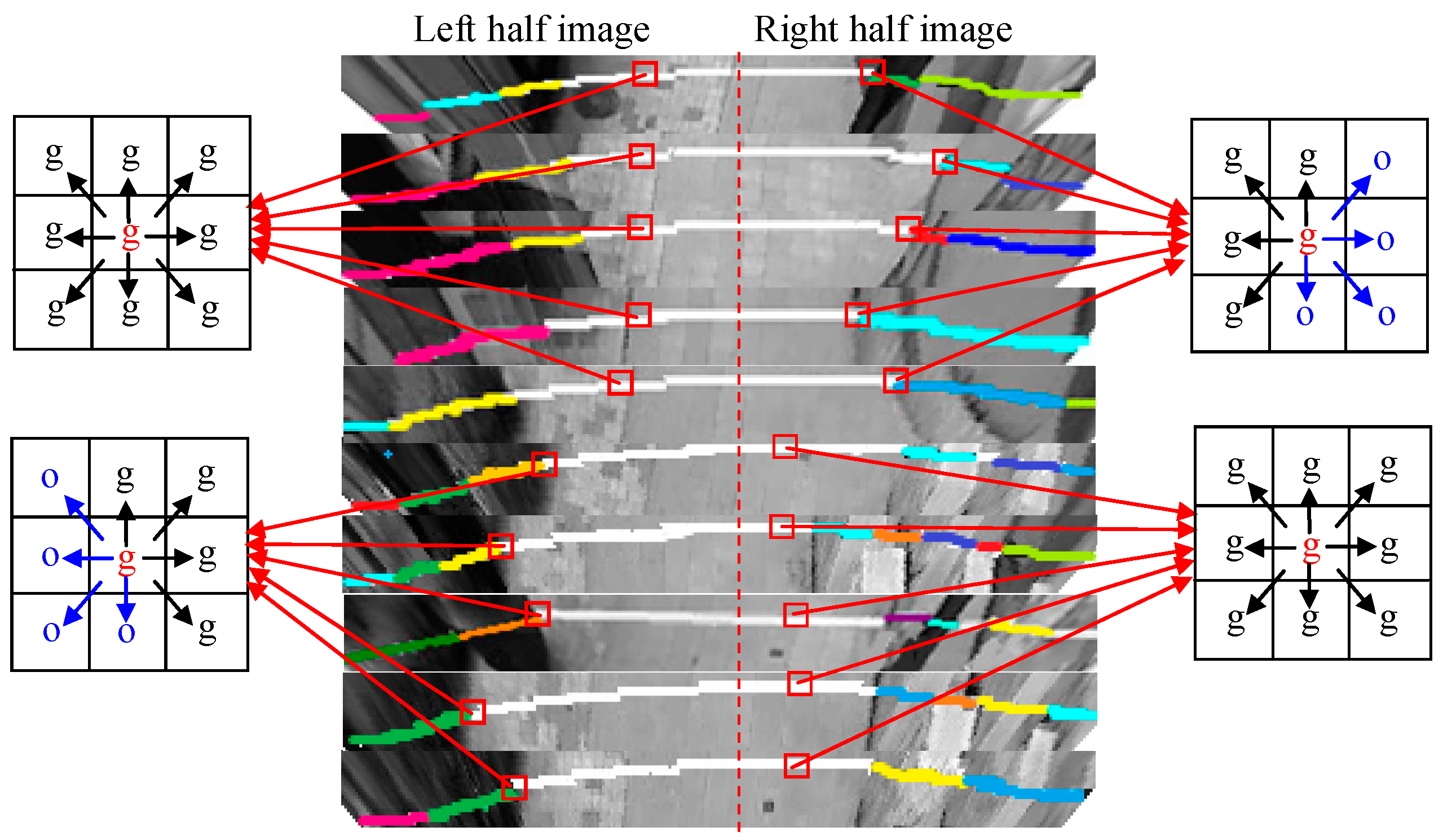
Figure 22d shows that the best performance is achieved by building spatial prototype in 1-pixel unit. And the neighbourhood histogram will deviate from the true spatial distribution when it is built using pixel groups. However, it takes a lot of computation cost for building and propagating spatial context in 1-pixel unit. Therefore, the 5 × 5 pixel group is used to achieve a balance between computation cost and interpretation performance.
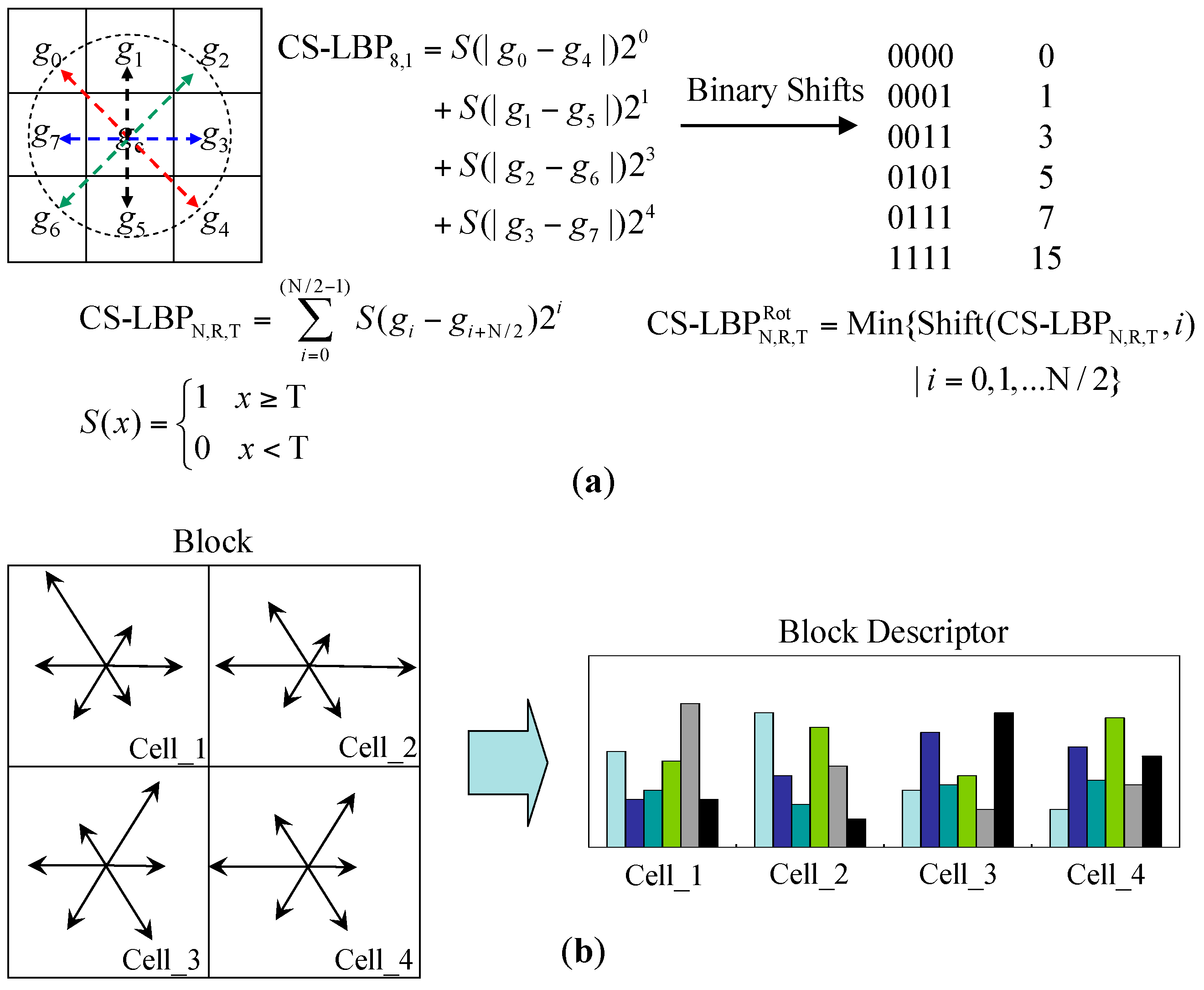
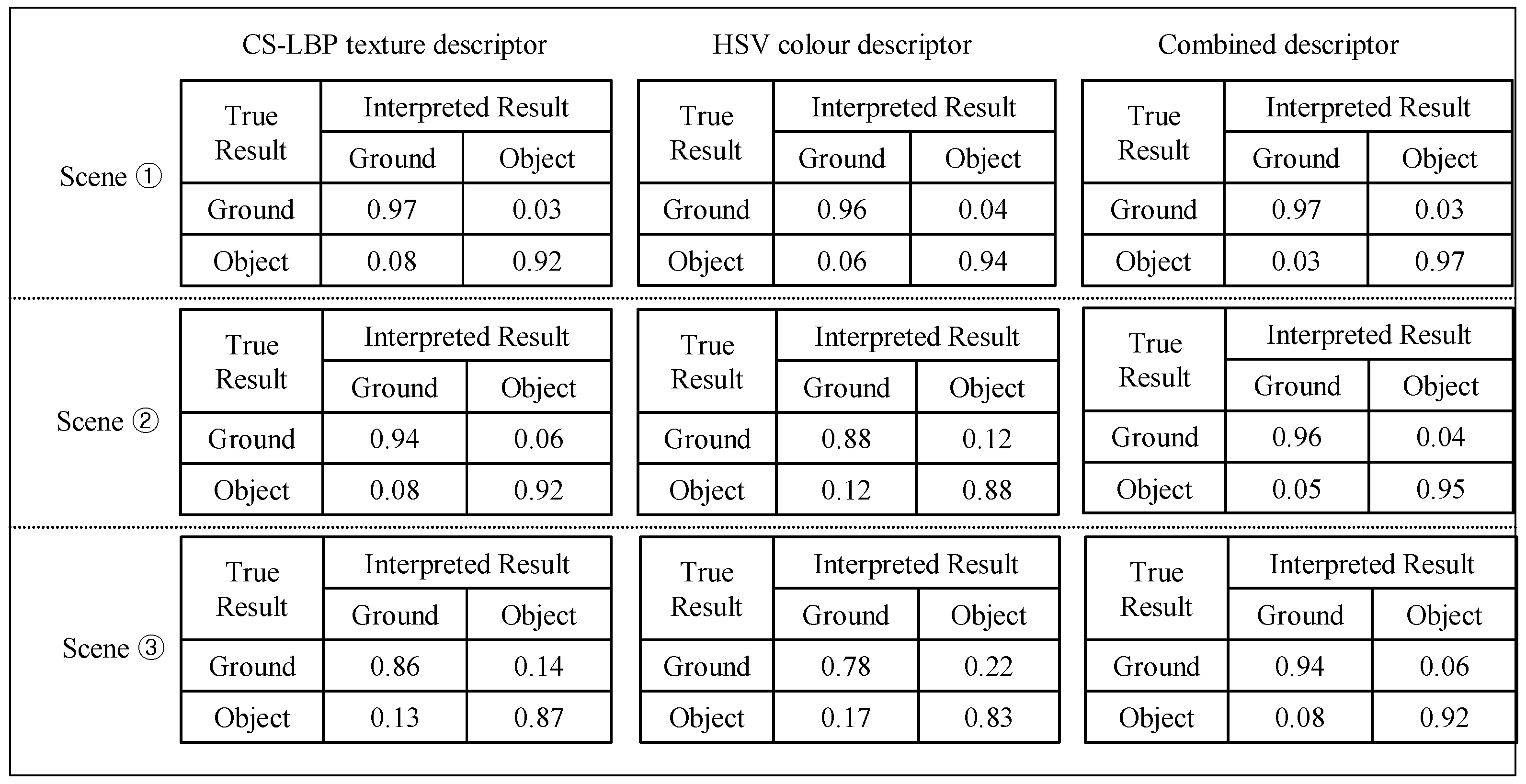
Finally, experiments are conducted on the interpretation performance regarding different types of descriptors. In one experiment, three types of appearance descriptors were applied to the sample images from the three test scenes; the average interpretation results are listed in
Figure 23. In
Figure 23, the first column shows the interpretation results obtained using only the CS-LBP descriptor, the second column shows the interpretation results of the colour histogram and the third column shows the interpretation results of the combined CS-LBP and colour histogram.
The interpretation results in
Figure 23 show that the CS-LBP descriptor and colour histogram descriptor may compensate for each other in the appearance interpretation. For example, in test scene ①, the texture of ground and roadside objects (low wall on the left) is similar, while the colour is very different. Therefore, the CS-LBP descriptor behaves worse than the colour histogram descriptor. While in test scene ②, the opposite is true. Therefore, the combined descriptor can produce better results compared to a single type of descriptor alone.
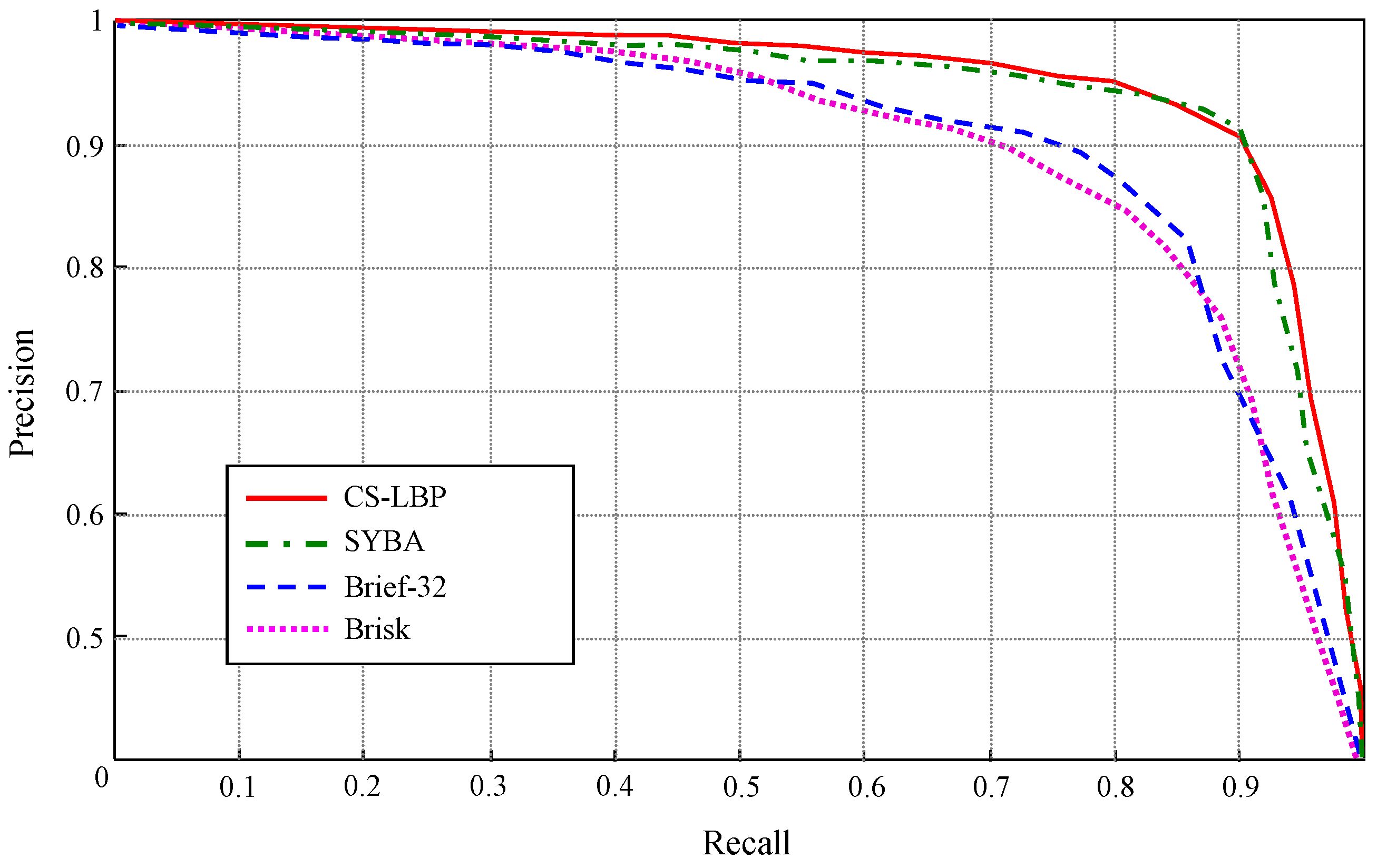
In another experiment, the far-field interpretation performance using different types of binary descriptors are compared as shown in
Figure 24. In this experiment, four types of binary descriptors are applied to the images in test scene ③, and the precision-recall curve of each binary descriptor is obtained by varying the decision threshold in a similar way that the ROC curves are obtained in
Figure 20. When building the ground prototype, the feature points are detected on the top-view domain using FAST detector for all the binary descriptors, and all the binary descriptors are applied to a canonical image block size of 32 × 32.
As shown in
Figure 24, CS-LBP and SYBA [
28] descriptor achieve similar performance. At 90% recall, both of them maintain high precision level above 92%. While for Brief [
29] and Brisk [
30], their precision fall below 74% at 90% recall. Therefore, CS-LBP and SYBA show better discrimination capabilities for the test scenes. The reasons for this performance difference are mainly due to the descriptor structure. The CS-LBP descriptor captures gradient patterns across the diagonal direction in a neighbourhood, and the gradient patterns are represented in histograms concatenated from adjacent cells. Therefore, local textures with their spatial distributions can be well encoded in CS-LBP descriptor. Similarly, SYBA descriptor encodes local texture and their spatial distributions by using synthetic basis functions. In comparison, Brief descriptor takes the gray level difference at random pixel locations to build a binary string as the descriptor. Although it is easy to build and compare, the binary string built in this way loses some statistical and spatial properties of local textures. Therefore, the performance of Brief descriptor might be sufficient for key point matching, but for the task of texture representation and classification, the CS-LBP and SYBA descriptors turn out to be better choices.
5.2. Run-Time Performance of the Dual-Field Sensing Model
Significant effort is invested in implementing the model to make the dual-field sensing model really work for real guidance tasks. Many strategies and techniques are applied in the implementation to achieve a balance between the interpretation performance and the run-time performance. The near-field model proposed in [
23] was re-implemented to allow sufficient run-time space for the far-field model computation.
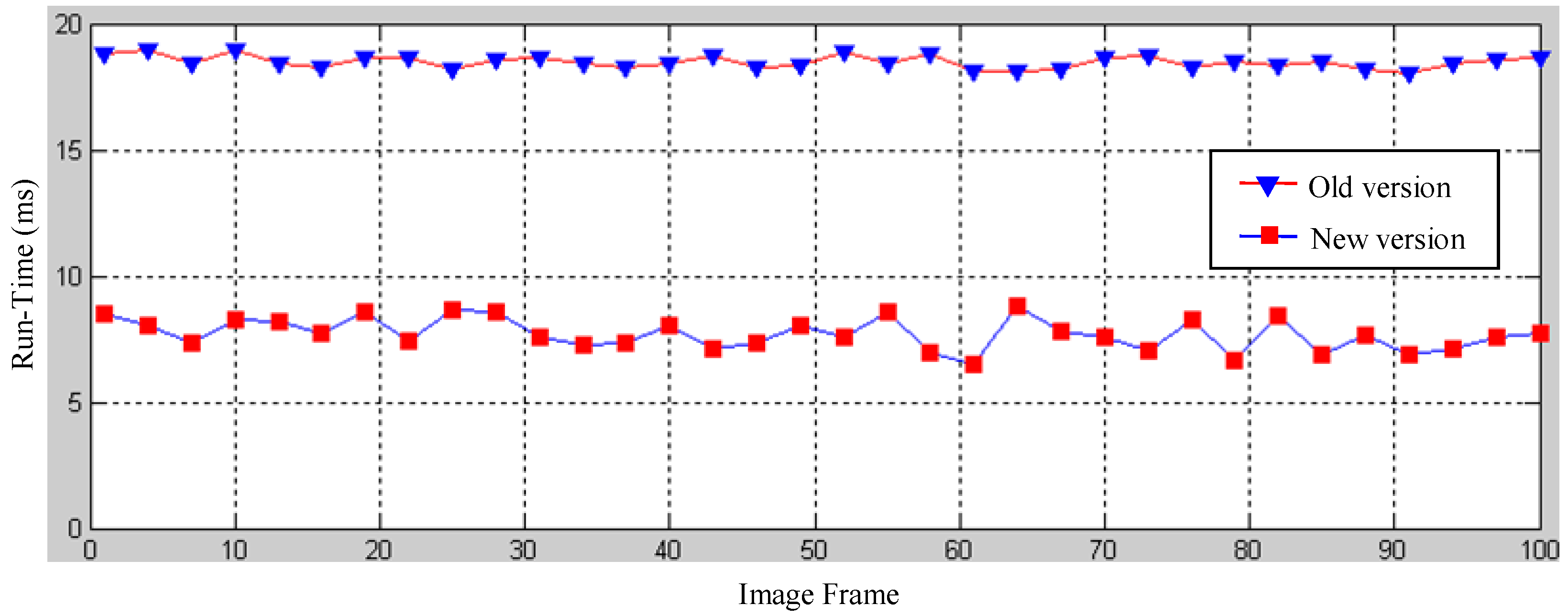
One of the major improvements in the near-field model is the implementation of a scout-point-voting scheme for object profile separation. In the old version, a gradient-ascend maximisation of a smooth likelihood function was required to separate range data into smooth object profiles. In the old version, each range data point has to be moved to one of the local maxima of the smooth likelihood function using a gradient-ascend vector. Scout-point-voting is based on the fact that the number of local maxima is generally far less than the number of laser points, and most local maxima can be identified by moving only a few scout points. For a regular point, its convergence destination is voted using the destinations of scout-points that pass by its neighbourhood. Therefore, the majority of laser-points can be directly assigned to its local maxima without doing a gradient-ascent computation. A run-time comparison of the old and new versions of the object profile clustering is shown in
Figure 25. It shows that the new version reduces the run-time to about half that of the old version using the scout-point voting scheme.
In the far-field model, the major implementation strategies used to optimise run-time performance are listed in
Table 3. In addition, an integration of a multi-core programming technique and a graphical processing unit (GPU) programming technique was also used in the implementation to fully exploit the maximum capacity of the computing platform.
Finally, to evaluate the run time performance of the dual-field model, an optimised implementation is run on a laptop computer with the specifications shown in
Table 4. The specification of the data frame is shown in
Table 5, and sensor data collected from the test scene ② shown in
Figure 19 are used to run this experiment. The model parameters are tuned to reach a balance between the interpretation accuracy and running time. The average run-time result for one data frame is listed in
Table 6. It took about 197.93 ms for the dual-field model to process one data frame. This runtime performance achieves about 5 frames per second on average.
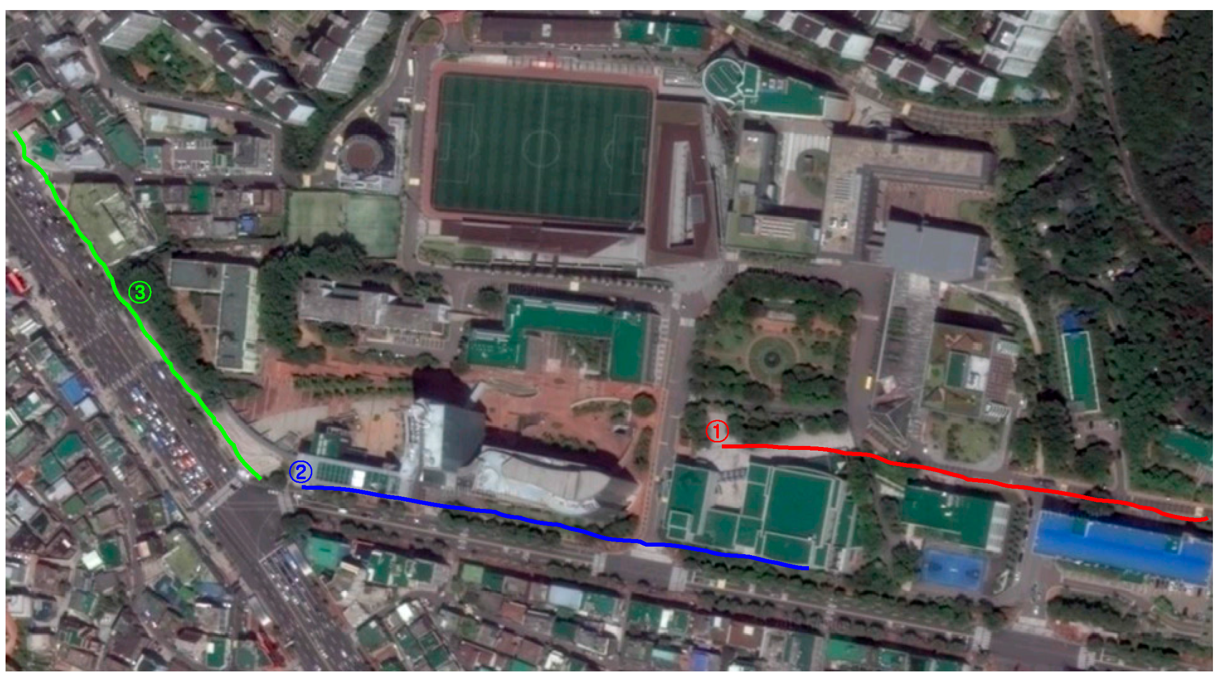
5.3. Guidance Performance of the Dual-Field Sensing Scheme
To test the guidance performance of the dual-field sensing scheme, three urban paths around our campus are selected for the field test. These testing paths are shown in
Figure 26, where path ① corresponds to test scene ① shown in
Figure 19, and paths ② and ③ correspond to test scenes ② and ③, respectively.
Each test path spans a length of 250 m. The blind users who participated in the field test were unfamiliar with the test paths. During testing, each blind user was asked to carry the whole guidance system on their body, including the sensor platform and the notebook computer. Each blind user was supposed to walk along the test path by following the guidance messages provided by the system. To test the efficiency of the dual-field sensing scheme, each field test was run three times. In the first round, the blind users were asked to walk along the path using only a white cane. In the second round, the blind users conducted the test using our guidance system with only near-field sensing. In the third round, the blind users were required to use the guidance system with the dual-field sensing.
The field test was performed at around 11:00 a.m. in the morning and at 4:00 p.m. in the afternoon when there was a moderate number of moving objects, such as pedestrians on the road. There were also various static objects located along the testing paths. The time it took for the blind user to walk along each path was recorded, and the average time it took to walk along each path is shown in
Figure 26.
Figure 27a shows that the guidance system dramatically reduces the time it takes to walk along each path, and the more complex the road condition is, the more efficient the guidance system is. On path ①, where the road environment is simple, there is not much difference between using a white cane and the guidance system. However, on paths ② and path ③, where road conditions are more complex, the dual-field sensing scheme demonstrates its efficiency. The increased efficiency is measured as |
tg-
tc|/
tc quantitatively, where
tg is the traveling time when using the guidance system, and
tc is the traveling time when using a white cane. The efficiency evaluation result is shown in
Figure 27b.
It can be observed that the dual-field sensing scheme provides extra efficiency compared to only near-field sensing. For example, on path ③, the near-field sensing module reduces the travelling time by 16.3%, and the dual-field sensing scheme reduces the travelling time by 34%. The field test results have proved the effectiveness of using the dual-field sensing scheme for guiding the blind people in an urban walking environment.


