Firstly, a general overview of the performance metrics is described followed by a revision of the different datasets used for the assessment of the algorithm and a detailed report of the results for each of the sequences.
4.1. Performance Metrics
This section presents the metrics used to evaluate the performance of our algorithm for different test sequences (motion captured or synthetically generated). After a sequence is processed by the algorithm, the output results are post-processed to compare the performance of the algorithm using the ground truth. The way that the sequences are adapted to our system is also explained.
We evaluate reconstruction error using the following indicators:
2D error:
where
F is the number of frames of the sequences,
P is the number of points,
are the re-projected features on the image and
represent the image coordinates of the ground-truth points.
3D error:
is the estimated shape and
the ground truth shape.
The 2D reprojection error and the 3D reconstruction error were defined in [
21]. When applied to an entire sequence, the error indicators are either averaged or presented individually for each frame. The former is useful to analyze the evolution of the error over time.
Regarding the 3D error, a previous Procrustes analysis [
68] is carried out before applying Equation (
30). It rotates and scales the shapes to align them w.r.t. the ground-truth. This is a common procedure in the state-of-the-art works, such as in [
12,
21]. Unless the opposite is explicitly indicated, this alignment is always applied before computing 3D errors.
4.2. Setup
In order to run the algorithm, we need a set of basis shapes, a rigid shape and an initial pose. These are estimated from the ground truth data as follows:
The rigid shape
is computed by extracting the average of the set of shapes used to obtain the bases. The initial pose is retrieved from the projection on the initial frame. We use PCA to retrieve the set of shape bases. The rigid shape is previously subtracted from the shapes, and no Procrustes alignment is applied before factorization. The basis shapes are then computed using PCA from this expression:
After PCA is computed from this matrix, the bases (
) are obtained, but only the
K most relevant components are taken. The number of bases used for all the experiments are at least
, unless the opposite is indicated. We always ensure that the value of
K represents at least 85% of the total deformation energy obtained from the PCA decomposition following the expressions in Equations (
32) and (
33). A higher number of bases can lead to over-fitting when dealing with real data, not to mention the memory and computational costs of handling a large number of bases. These are the main reasons why a fixed value (unless specified) of bases is set.
It must be noted that no Procrustes alignment is applied before the SVD factorization.
To handle the data from motion captured datasets, without any kind of visual information, a special version of the tracking thread is developed, to accept as input text files containing the point projections for each frame, the 3D bases, the pose initialization, the visibility masks, etc. The ground truth 3D points are projected using the perspective camera (Equation (
3)), choosing a convenient pose to see all the sequence points over time.
To perform a thorough comparison and to simulate real tracking conditions for these datasets, the following sets of outlier percentage values
% and noise strength values
are added to the set of projected points. This is similar to the evaluation proposed in [
53]. With this setup, an initial evaluation is performed to check the tracking robustness under these conditions. The added noise follows a normal distribution
. A percentage of the image points is marked as outliers. For those points both spacial directions are randomly deviated 20 pixels. Point visibility is also introduced as a variable to analyze algorithm robustness. To that end, randomly distributed visibility masks in an increasing percentage are generated.
All the experiments are computed using an i7 laptop with 8 GB RAM and eight virtual core processor at 2.4 GHz. The algorithm is implemented in C++ and runs on Ubuntu Linux, using PTAM-derived libraries, OpenMP, CGAL and OpenCV. If it is not specified, the tests for the methods of [
11,
12,
20,
21] are executed with the default parameters given by the authors. We set the motion movement constant
to 0.9; the radius limit of the IROS-based feature detection is 30 px; and the one for the rest of the matching algorithms is 70 px.
A general overview of the algorithm performance is presented with two motion capture datasets. We start evaluating the tracking with the assumption that the matching is perfect. After that, the results are re-evaluated for tracking under visibility degradation, noise, outliers and varying the number of basis shapes. Smoothing priors are not included in these experiments.
For real images, we analyze the performance by testing some matching methods, varying the number of basis shapes, and finally, we analyze the performance using the smoothing priors. Using real images implies that missing data, outliers and noise are already present in the data.
4.3. Flag Sequence
A motion captured flag bending with the wind is represented in the flag sequence. The deformations are so significant that they make this dataset challenging. Moreover, the amount of points in the sequence (540 in 450 frames projected on 640 × 480 images) is significantly higher than in other synthetic datasets used in the state-of-the-art, which implies a challenge to factorization-based algorithms. The deformation energy kept by the first 15 bases () is 87.33%, which follows the imposed criteria of keeping 85% of the deformation energy.
4.3.1. Performance Evaluation Based on Perfect Matching
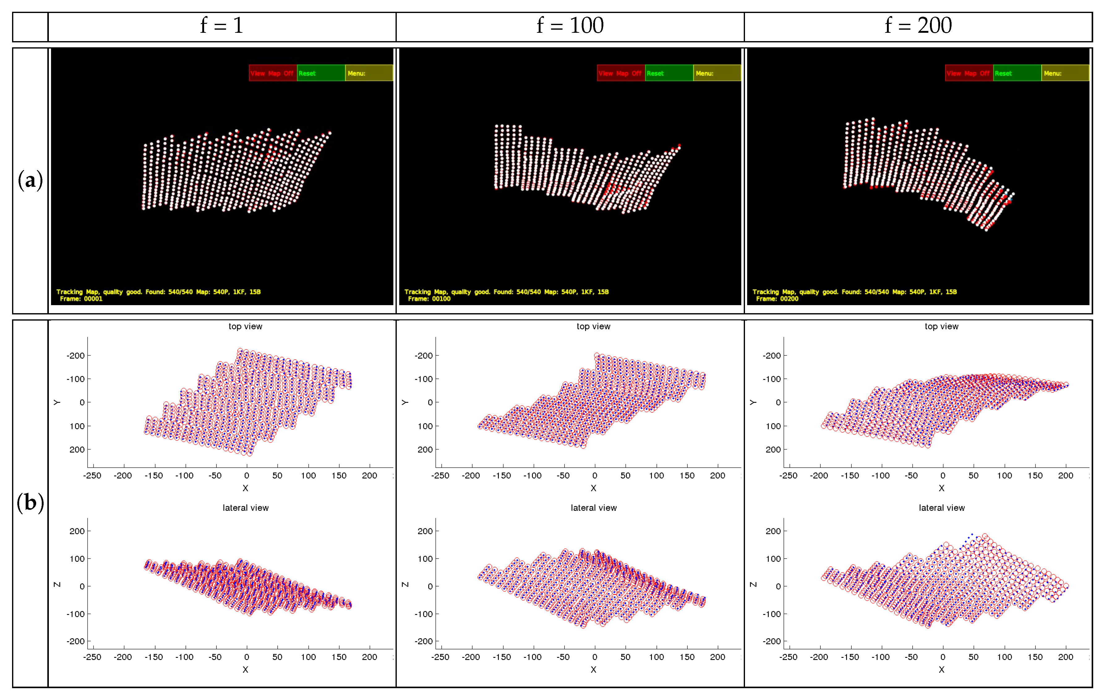
Some examples of both sequences are shown in
Figure 3a. 3D reconstruction results without any degradation on the matching are shown in
Figure 3b. They are compared to the ground truth, which is represented in blue, whilst the reconstruction result is represented in red. Two views are shown to better display the 3D reconstruction. For most of the frames, the reconstruction is very accurate. The average performance is shown in the row for
bases shown in
Table 1.
In Frame #200, the reconstruction result shows more error on one of the corners, which corresponds to high frequency deformations that might not have been properly modeled. The results can be improved, in this case of perfect matching, by increasing the number of bases.
The reprojection and reconstruction errors for a perfect matching over time are shown in
Figure 4. Increasing the number of bases minimizes these errors, as will be seen in
Section 4.3.4. However, as will be discussed in
Section 4.6.2, this trend will not be valid when correspondences are obtained with the matching of real images.
4.3.2. Performance Evaluation Based on Visibility Degradation
Missing detection of features is simulated by using visibility masks. These masks are generated according to a percentage of missing data. The visibility distribution of the masks for each point and among frames follows a uniform random distribution.
Some results within a range of visibility from 5%–100% are carried out. The 2D reprojection and the 3D reconstruction errors are computed for both sequences. For the flag sequence, the errors are stable from 20–100%, which represents a minimum of 108 points. They have the following values on average: two pixels for 2D reprojection error and 2.6% for 3D reconstruction error. We highlight that the visibility distribution follows here a random uniform distribution. In real images, missing data usually affect entire areas of the image, due to occlusions or lack of texture. In some detectors, the visibility percentage varies from 50%–30%.
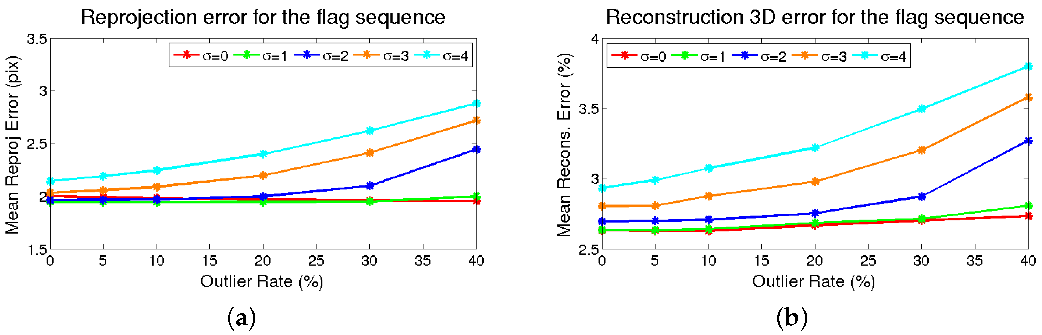
4.3.3. Performance Evaluation Based on Noise and Outliers
Similarly to the previous test, robustness analysis due to outliers and noise is performed. Different values for noise and outliers have been evaluated, as mentioned in
Section 4.1. The experiments are repeated 10 times, and the average is taken, to achieve representative results, as a standard Monte Carlo experiment.
The results are shown in
Figure 5. It can be seen that the 2D reprojection error is not significantly increased for the lowest
values as the number of the outliers grows, meaning that the M-estimator is capable of dealing with them.For higher values of
, the error gap between the methods is approximately the same as the number of outliers increases, the limit being
. With respect to the 3D reconstruction error, the trend is the same as in 2D reprojection error, starting at 2.6%.
4.3.4. Performance Evaluation Based on the Number of Bases
The dependence of the accuracy results with the number of bases is checked as well. For that purpose, a test using tracks without degradation and with 5, 7, 15, 25 and 30 bases is presented in
Table 1.
Using perfect matching, as the number of bases increases, the error decreases for the presented sequence and so do all the error indicators. In addition, the processing time improves as the number of bases is reduced, as well as the memory requirements.
4.3.5. Comparison with Other Methods of the State-Of-The-Art
Table 2 shows a summary of results with the most representative methods of the state-of-the-art for the flag sequence. Processing time for the whole sequence, 3D accuracy, 2D error, rank, modeling type (auto/a priori) and procedure type (batch/sequential) are depicted. In this case, our algorithm gets close to the best ones in terms of 3D accuracy and 2D reprojection error for this sequence. In our approach, no priors are applied, in contrast to the best ones, in which physical priors such as isometry [
34] or partial modeling [
42] are used. Our approach can be better compared with sequential algorithms [
21,
24], as the estimation scheme follows a similar (sequential) approach. Regarding [
21], our algorithm outperforms their 2D and 3D error. With respect to [
24], our algorithm obtains comparable results using a lower amount of bases and without physical priors.
Regarding computation times, our algorithm is the best among all compared methods, thus reaching the best trade-off between performance and processing time. However, it must be highlighted that some of the competing methods are not optimized to run in real time, and some of them are implemented in MATLAB, while our method is implemented and optimized in C++.
The trials of [
44,
69] did not finish processing the sequence after the referenced time. For some of the methods, where the source code is available [
11,
12,
20,
21,
44,
69], the same hardware is used to run the experiments. In [
69], they provide results with this dataset. We present them in a second column inside the 3D error column as we found some discrepancy betweenour tests and the ones provided in the original paper.
Algorithms where the code and processing times are not available, such as the results of [
34,
42], are not reported in
Table 2. Batch algorithms implemented in MATLAB such as [
11,
12,
20,
21,
24,
44,
69] take more time than those developed in the C++ language, like [
40]. A C++ implementation does not automatically imply real-time performance, as the code needs to be optimized, but also the data volume needs to be restricted to be properly handled in real time.
Comparing the MATLAB processing time in
Table 2 and
Table 3, it gives an idea of the complexity of the flag dataset.
Table 2 shows that current solutions based on model-free methods (NRSfM) cannot recover the correct 3D shape for the flag sequence with a non-normalized error, unless the approach includes some extra prior (we recommend to the readers the review of [
69]). As our method is model-based, it provides acceptable error values and is faster than the rest of model-free approaches, reaching 70–90 fps, which is compatible with real-time constraints. It must be noted that no visual information processing is applied in any of the tested approaches.
4.4. CMUfaceSequence
This sequence presents a face of a person while changing the pose and talking. This sequence is used in other methods such as in [
21]. The sequence is mostly subject to rigid motions, although it presents deformations on the mouth area, when the person is talking. The amount of points is 40 over 315 frames projected on an image size of 640 × 480. The deformation energy kept by the first 15 bases (
) is 95.8%, which follows the minimum energy criteria explained in
Section 4.2.
The same tests have been carried out for this sequence, and the same trends observed in previous experiments have been seen here. As the number of points is significantly fewer than in the flag sequence, the minimum amount of points to consider for visibility is 50%. The same trend and conclusions can be extracted for the analysis with noise, outliers and bases, only varying the average values. The average value for K = 15 bases is 0.26 for 2D reprojection error and 1% of 3D reconstruction error.
Table 3 shows a summary of the results obtained with the CMUfacecompared to the sparse approaches [
11,
12,
20,
21]. The same format as in
Table 2 is used. In this case, the presented algorithm gets the best results among the tested algorithms for the error parameters and the time performance.
In a sequence in which most of the behavior is rigid except for the mouth movements, the overall performance of the algorithms is good as they all exploit this circumstance. The presented model-based reconstruction algorithm outperforms the results of model-free approaches.
4.5. Point-Wise CVLab’s Kinect Paper
This dataset is derived from the Kinect paper dataset presented in [
70]. It consists of a video sequence of 99 points on 191 frames showing a deforming piece of paper, which is captured with a depth sensor. The projections of the mesh for each frame have been obtained by interpolation from the set of original matches. The projections are further adjusted by estimating the relative camera-object pose and making sure that they match with the original SIFT images.
We see the same trend observed in the previous datasets when the number of bases is incremented. This dataset needs a bigger amount of bases to achieve good reconstruction results. For K = 15, the 2D error is about 9 px, and the 3D error almost reaches 11.92%, whereas, for K = 80, the 2D error becomes lower (8 px approximately), and the 3D error goes to 11.8%.
4.6. Rendered Flag Sequence
The flag sequence depicted in the previous tests is interpolated to get a dense surface and then is rendered using orthographic projection, as presented in [
71]. As our model-based tracking works with the perspective projection, this sequence was re-rendered with perspective projection. The sequence contains 450 frames.
This sequence was chosen in other works [
24,
43,
52,
71] as it consists of a set of images and a dense 3D ground truth to evaluate the performance of tracking methods. It is useful for our experiments because, even though our tracking is sparse, the ground truth is appropriate to perform a thorough comparison among different methods.
4.6.1. Evaluation of Visual Descriptors
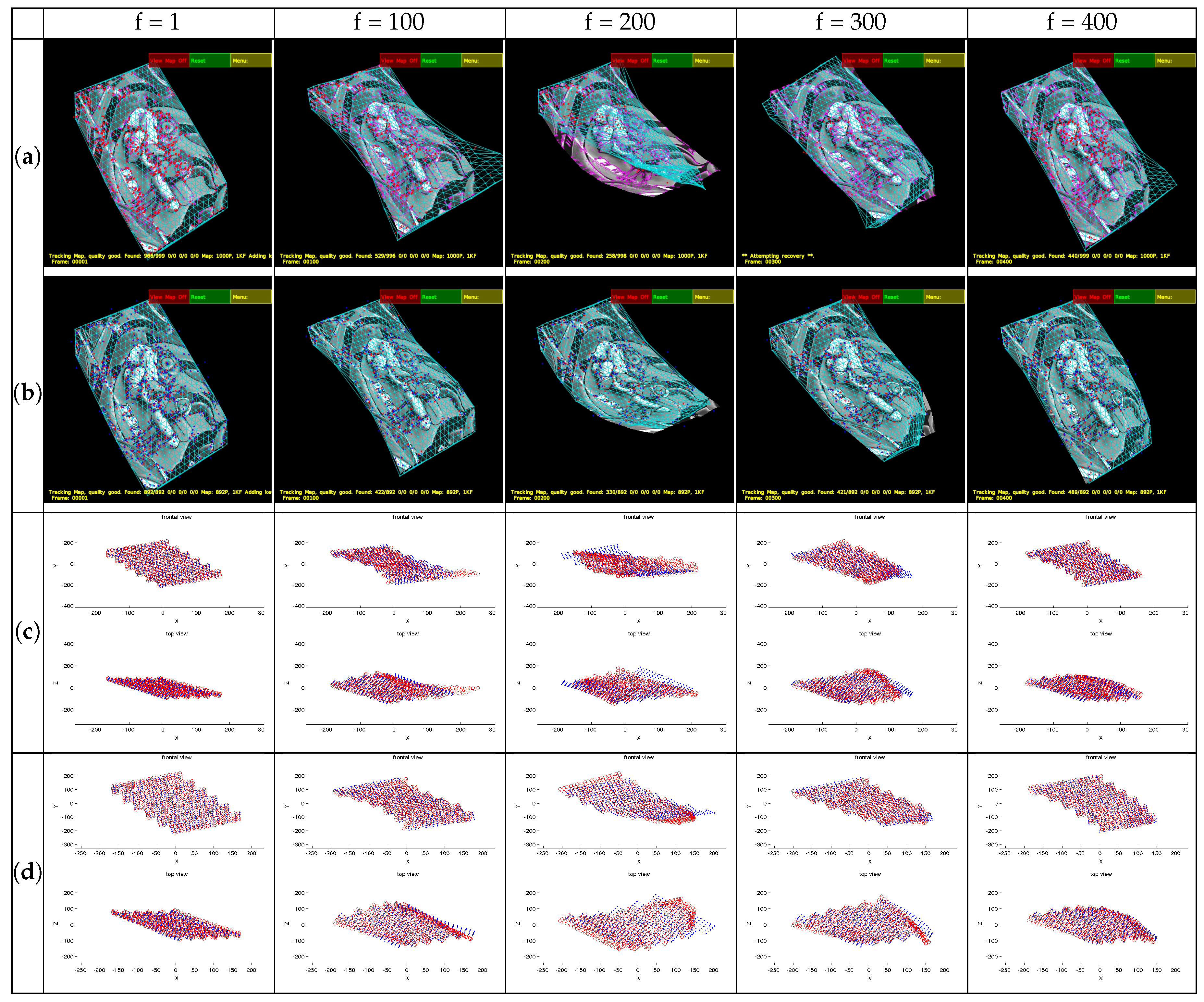
First of all, some frames of the sequence processed with the IROS-based tracking published by the authors in [
52] are shown in
Figure 6a together with reconstructions (
Figure 6c). The same frames processed with the SIFT tracking and their reconstructions are shown in
Figure 6b,d. The detected points (
Figure 6a,b is shown in magenta, the matched points in red, and the mesh model is overlaid in cyan, to give an idea of the tracking performance. Regarding the 3D reconstructions (
Figure 6c,d), the ground truth points are represented in blue and the reconstruction in red.
In our method, the feature detection and matching methods are configured to prioritize speed over accuracy. The frames are ordered in the columns and the tracking methods in the rows. It can be seen that in Frame #200, there are some accuracy problems for the presented approaches. This is due to the sequence presenting very abrupt movements combined with an interval of possible tracking losses. The detection of features in these areas is a difficult task, even for the most advanced feature descriptors, so there are very few points detected in this area, yielding a poor local estimation.
The projection of the model on the screenshots (cyan) and the reconstruction results differ because the shape in the latter is obtained after applying Procrustes alignment between the ground truth and the reconstruction.
In order to have a general performance overview for all the analyzed descriptors, a benchmark is shown in
Table 4. This comparative includes number of points, descriptor, matcher, processing time (for the whole sequence and fps), 2D error and 3D error.
A similar benchmark, but including the matching technique used for each feature descriptor, is shown in
Figure 7. This studies the influence of the matching method on the error metrics. For binary descriptors such as AKAZE, ORB and BRISK, the use of Hamming distance slightly improves the results of 2D reprojection and 3D reconstruction.
Figure 7 shows that the best method according to the reprojection error is not necessarily the best in terms of the reconstruction error, as we pointed out before. SIFT gets the best performance for both error estimations and among all the matching algorithms (brute force L1, L2). However, the second best is not the same for both figures (SURF in 2D and AKAZE in 3D).
AKAZE performs almost as well as SURF in terms of 2D reprojection error and is almost as good as SIFT in terms of 3D reconstruction error. Looking at
Table 4, it can be seen that AKAZE is also one of the fastest approaches, which makes it a good candidate for a final implementation.
Regarding this table, it can be seen that the fastest approaches are IROS, AKAZE, ORB and SURF, and the ones that handle the most points are IROS, BRISK, ORB and SIFT. We remind that state-of-the-art approaches are only capable of working with a very small amount of points obtained from interpolated models. In this case, all the detected points are used to perform the estimation. It is important to remark that most of the reported time is consumed by the feature detection algorithm. The obtained times show the influence of the visual processing, compared with the reported results on the flag sequence in
Table 2, in which the visual detection stage is not applied. PTAM results are included as a baseline for rigid SfM.
4.6.2. Performance Evaluation Based on the Number of Bases
As was done previously with the point-wise flag sequence dataset, the influence of the number of bases is tested for real conditions.
We show averaged results in
Table 5. It can be seen that the trend observed with ideal matching is reversed here. Increasing the number of bases does not necessarily increases the 3D error. For IROS-based and SIFT-based tracking, the best results are obtained for seven bases.
This clearly means that with real matches, the DoF of the shape model plays an important role in the reconstruction accuracy. With more bases, the model becomes more capable of adapting to large matching errors and more prone to erroneous reconstructions in areas of the object with a small amount of detected points. This effect is fixed by introducing priors as we explain in the next section and as displayed in
Table 6.
4.6.3. Performance Evaluation with Time and Shape Smoothing Priors
Working with real images increases uncertainty in matching, which causes ambiguities and errors in the 3D shape. In order to reduce these effects, priors must be added. Due to the nature of our optimization algorithm (linear and split), time and shape smoothness priors can be implemented. The priors are studied at three levels, depending on the strength at which they are imposed, which corresponds to the value of their hyperparameters in the optimization (low, medium and high). The values for each type of prior are obtained heuristically.
The SIFT descriptor is chosen for the matching, as it obtained the best performance results in our previous tests (
Table 4). Then, the results are compared to the IROS approach because it serves as a baseline of our first implementation [
52].
After 3D reconstructions and 2D projections have been studied, a temporal analysis of the tracking for both priors regarding the baseline without priors is carried out.
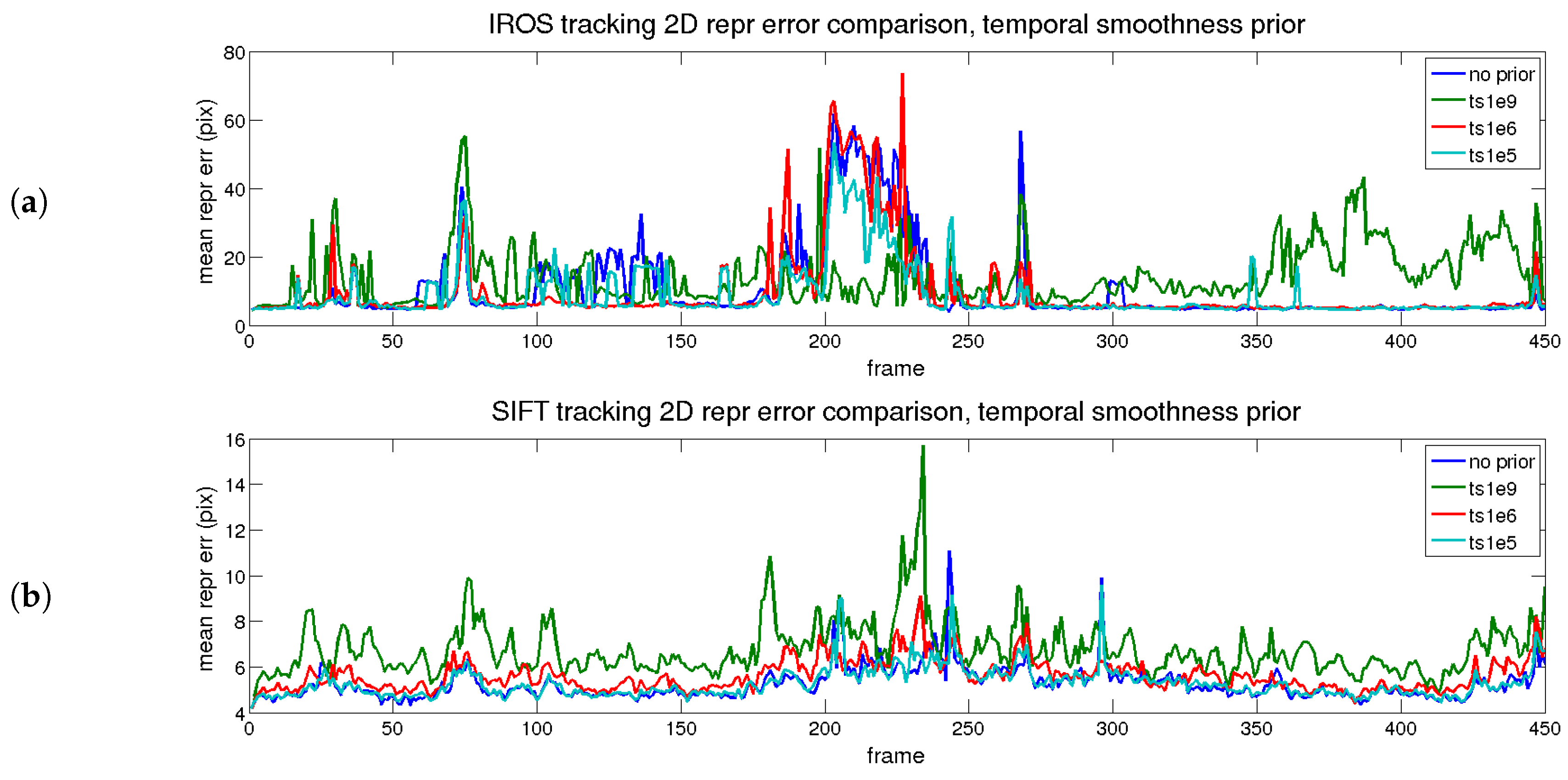
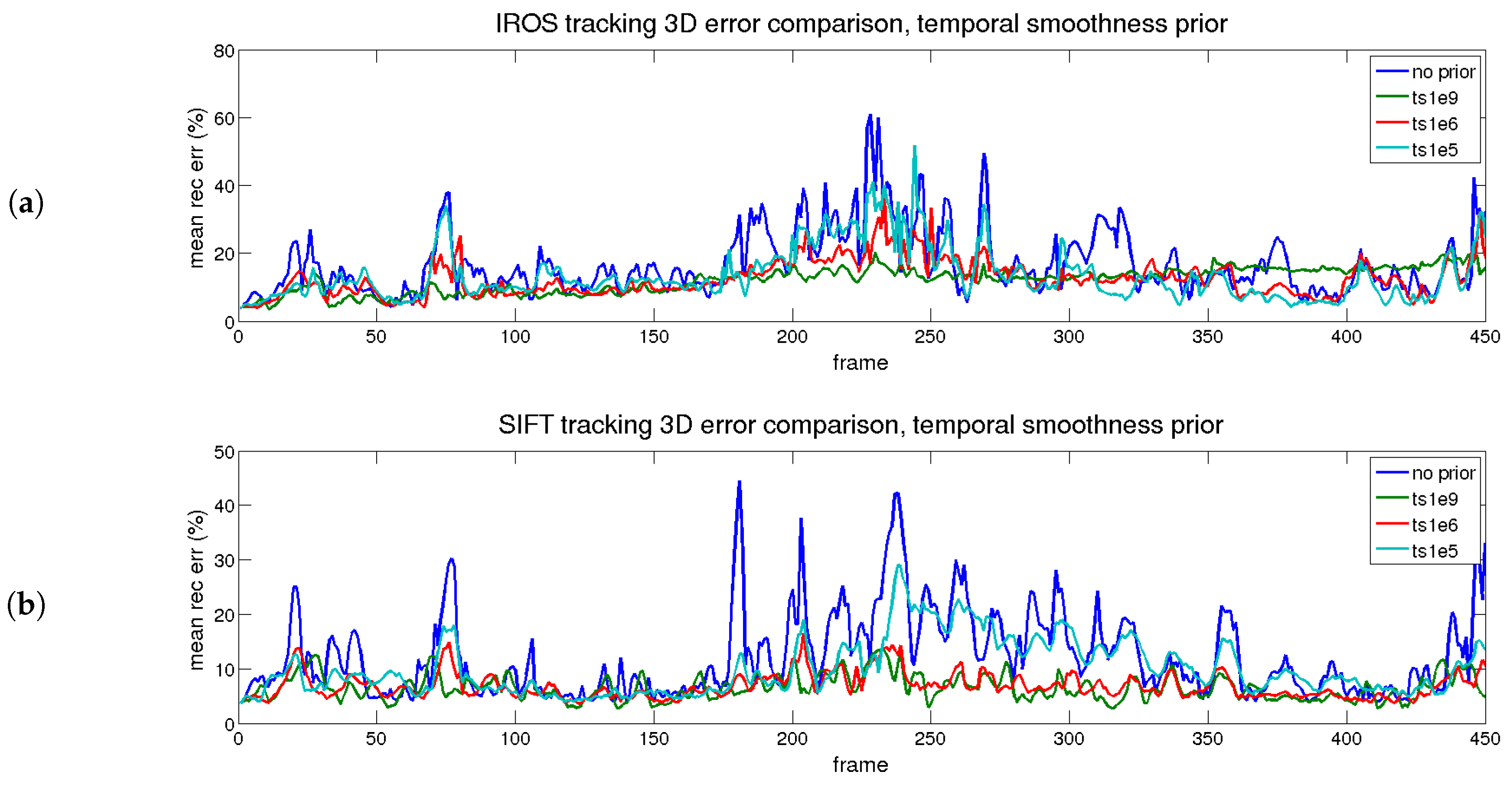
The first evaluated prior is time smoothness, depicting the errors shown in
Figure 8 and
Figure 9, which correspond to reprojection and 3D reconstruction errors. The figures are divided into two parts: the upper part corresponds to the IROS tracking, whereas the lower part corresponds to the SIFT tracking.
In
Figure 8, the reprojection errors are presented for the different priors with different colors. The blue trace represents the result without priors. In terms of error, cyan (low) and red (medium) traces are close to the blue trace. The green trace (high) presents high error for both approaches, except when the tracking is lost, as an excessive value of the prior makes the shape too rigid. The cyan trace, as expected, has little effect on the reprojection error, as the regularization value is low. The red trace has a slightly higher reprojection error, although in general terms, it is maintained along the sequence. Therefore, for the reprojection error, the prior does not imply an improvement.
The beneficial effect of the prior is seen in terms of reconstruction error, shown in
Figure 9. For both approaches, when the prior is applied (even for small values), the 3D reconstruction error is reduced.
The best option corresponds to the red trace (medium) for both approaches. In that case, the increment in the reprojection error is small and the improvement in the 3D reconstruction error is large with respect to the blue trace (no priors applied). The effect is even more noticeable when the tracking is better, comparing the IROS and SIFT approaches.
To sum up, the errors reached after applying different priors are depicted in
Table 6. The best results for each prior are marked in bold.The best option is obtained for a combination of both priors with medium values.
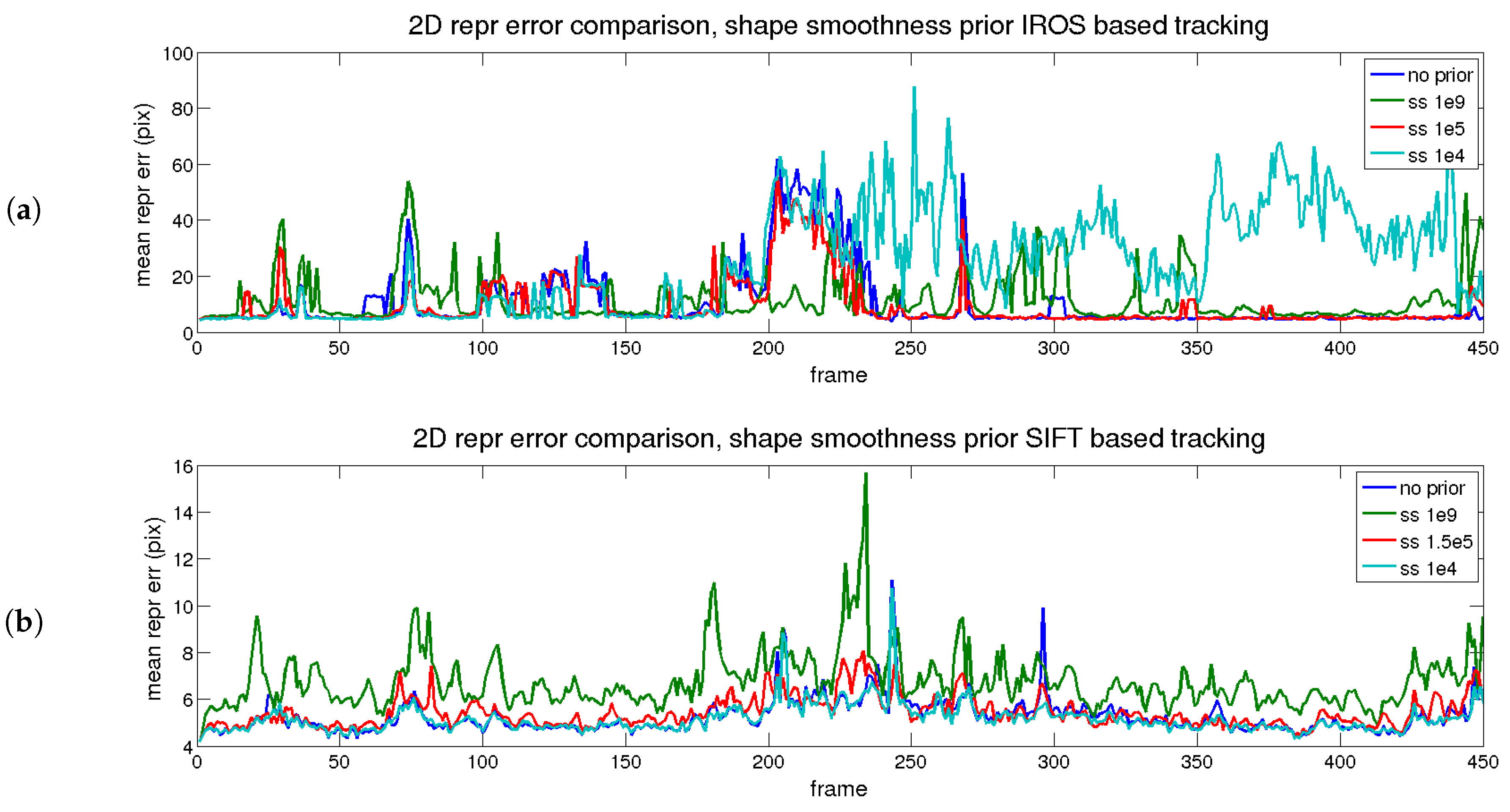
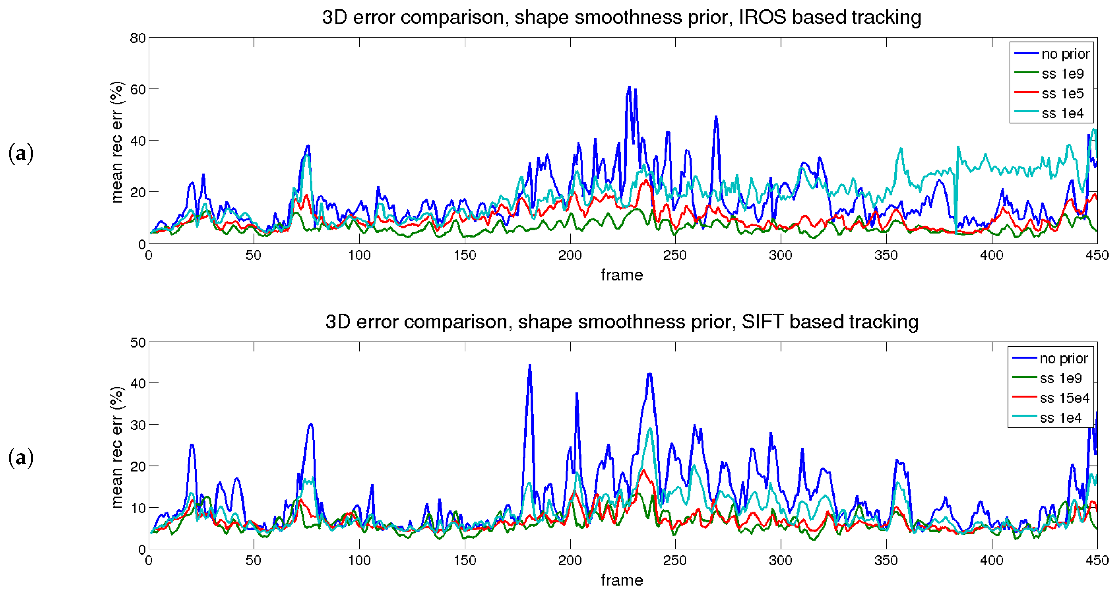
The results of the temporal analysis for the shape smoothness prior are depicted in
Figure 10 (reprojection) and
Figure 11 (3D reconstruction). A similar conclusion to the temporal smoothness prior can be extracted in this case. The trace in red (medium) reflects an equilibrium between reprojection and reconstruction errors, for both matching methods (IROS- and SIFT-based).
PTAM results are included to have a rigid SfM baseline in this sequence. On the other hand, just on the row below, the results from the (point-wise) flag sequence with perfect matching (
Table 2) are displayed to show the impact of dealing with real images.
According to
Table 6, the difference between the IROS and SIFT approaches is easy to explain: tracking quality is decisive to get accurate results, as the 2D reprojection error is about 4.3 pixels lower for SIFT before priors’ application. Regarding the 3D reconstruction error, it is about 4% lower (16 down to 12) before priors, and after priors, it is reduced an additional 3% with respect to the best mark (9 down to 6).
Processing time due to the addition of priors is not included in the table, because it does not add a substantial change.
4.7. CVLab’s Kinect Paper
This sequence was first proposed in [
70]. It consists of 191 frames of a well-textured piece of paper undergoing deformations and pose changes. The dataset includes a dense ground truth for each frame in the sequence. These data are acquired using the Kinect sensor, commonly used to test SfT algorithms.
One of the main differences of this sequence compared to the rendered flag is that, in this case, the background contains texture. Therefore, the area of the object is segmented at the beginning of the sequence to reject background features.
Regarding the results, they are similar to the ones in the rendered flag sequence. As the number of bases is increased, the 2D error is reduced, and the 3D error is increased. This time, there are few differences between the results using IROS and SIFT matching, as we show in
Table 7.
The results are this time slightly better for the IROS approach compared to SIFT as the search radius is greater in the latter. The possibility of having incorrect matches due to a bigger radius is increased even though SIFT matching is better.
Finally, a comparative table with other state-of-the-art algorithms is shown in
Table 8. We show our results without smoothing priors, which is a conservative result (check
Table 7). It can be seen that our results are comparable with those obtained in [
72].


