2.1. Principles of IGNS
For IGNS, the variation characteristics of an information database composed of high-resolution gravity reference maps were used to acquire the carrier location information [
16,
17]. Gravity matching-aided navigation primarily uses a variety of methods to compare the gravity values obtained using marine gravimeters and those stored in reference maps, thereby determining the optimal matching point according to the degree of fit between the two types of gravity values. Algorithms of gravity matching-aided navigation can largely be divided into two types, i.e., related matching algorithms represented by terrain contour matching (TERCOM) [
18,
19] and interactive closest contour point (ICCP) [
20], and multi-model Kalman filtering algorithms represented by the Sandia inertial terrain-aided navigation (SITAN) [
21,
22]. There are other algorithms, such as neural networks and particle filtering [
23,
24,
25]. Unlike the related matching algorithms, SITAN uses recursive Kalman filtering to calculate the carrier location in real time. It is insensitive to speed or heading errors and allows the carrier to move flexibly. Therefore, the SITAN algorithm was used in the following ocean experiment and simulation.
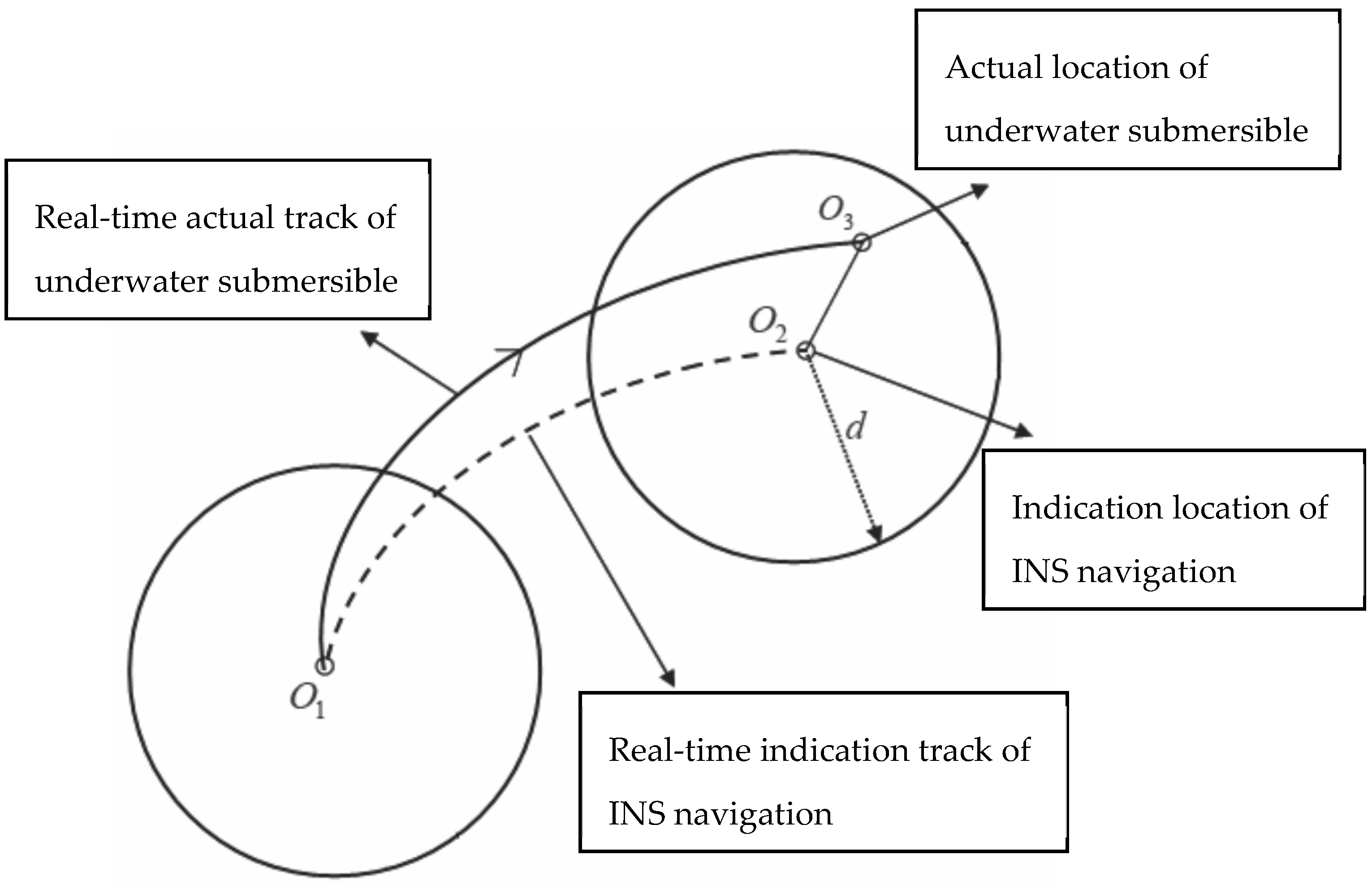
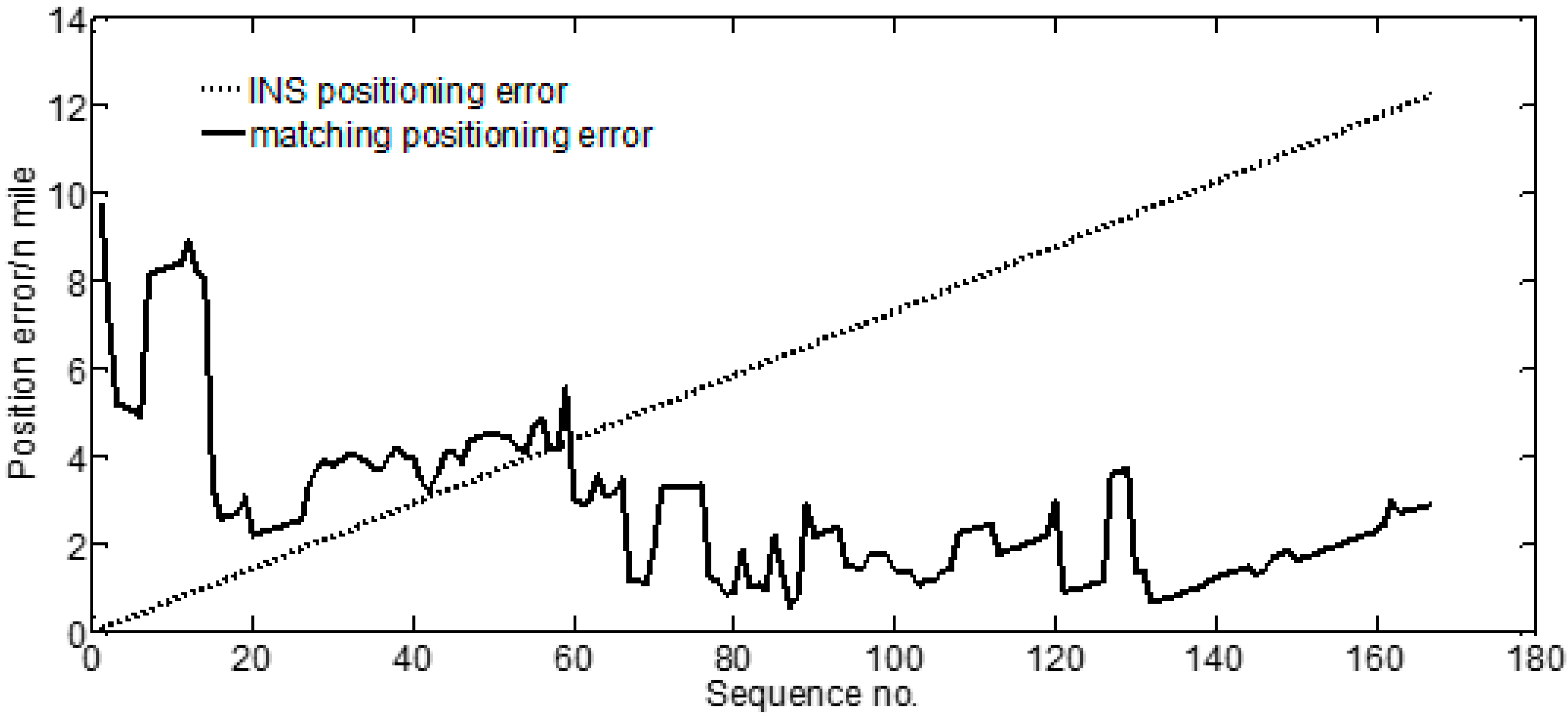
Figure 1 shows the drift of the INS locations with respect to the actual ones. If an underwater submersible sails from
to
, the INS location at this moment corresponding to the actual location
is
, because of the accumulated INS location error. The SITAN algorithm for gravity matching-aided navigation has two phases, namely, search and tracking. In the search phase, centered on location
indicated by the INS, the actual location area having a search radius
of the underwater submersible with 99% confidence was determined on an existing gravity anomaly reference map, based on the INS location accuracy and the circular error probability (CEP). With location
indicated by the INS as the center of the confidence area, a set of parallel Kalman filters was established in the confidence area to track and calculate the matched locations. These filters were ordered grids that had spacing consistent with the grid resolution of the gravity anomaly reference maps. The corresponding gravity anomaly interpolation was determined from the gravity anomaly reference maps on the basis of the filter distribution. The difference between the gravity anomaly interpolated from a reference map and that observed using a marine gravimeter was considered the measured value, ultimately forming the state equation and the measurement equation (see Equation (1)). The estimated gravity anomaly and location information along the route were obtained using Kalman filtering.
The state equation and the measurement equation of Kalman filtering in IGNS were constructed as follows [
26,
27]:
If we assume
,
is the observed value of the measurement equation at time
. Here,
denotes the gravity anomaly observed by the marine gravimeter, and
denotes the gravity anomaly interpolated from a reference map according to the INS-indicated locations. The state noise
and the measurement noise
are unrelated zero-mean white-noise sequences. Further,
is the system noise and
is the measurement noise.
After Kalman filtering with multiple groups of filters in the confidence area, an estimated gravity anomaly
was obtained for each group of filter. Then, each corresponding matched location was calculated. According to the Heli/SITAN algorithm [
28], the degree of fit was best reflected by the difference
between the measured and the estimated value. The residual
could be expressed as dollows:
The smoothed weighted residual square (SWRS) that reflects the effect of multiple filtering was constructed on the basis of the residual. Then, the location corresponding to the filter with the minimum SWRS was the optimal one. Here,
denotes a smoothed weighted factor (
).
is the estimated variance during the implementation of the Kalman filtering model, as shown by Equations (4) and (5).
Upon the Kalman filtering of the multiple sets of filters in the confidence area, we obtained the estimated location for each set of filters. According to Equation (5), the smaller the SWRS value is, the better is the matching effect. Among the positions of the filters with different SWRS values in the confidence area, the position corresponding to the filter with the smallest SWRS value was the optimal matching position. The reliability of this optimal matching position was judged using the following criterion:
where
denotes the smallest value of all of the filters in the entire confidence region,
indicates the smallest value of
beyond a certain range with
as the center,
represents the judgment criterion parameter, and
refers to the threshold. A large value of
indicates significant differences between the
and the
, and the larger the value is, the more prominent are the characteristics of the location corresponding to
. Therefore, the filter with
is regarded as the optimal estimation filter, and the optimal matching location corresponding to
is considered the effective location.
Considering the change in the marine gravity anomaly with distance, we found that the effective matching points had a typical spacing of 1–2 grids. The value function obtained using Equation (5) was the minimum, and the optimal location of the underwater carrier was localized on the gravity anomaly reference map. The matching location accuracy was considerably affected by the reference map resolution. In theory, the optimal matched location could be narrowed to 1 or even 1/2 of the gravity anomaly grid. In fact, when the gravity anomalies of 1 grid change were so small that they were overlaid by the noise of the gravity reference map error and of the gravimeter observations, we required 2–3 grids or a greater distance to ensure that the variation of the gravity anomaly met the requirement of high-precision matching and location determination. In the SITAN algorithm, the primary role of INS was to define a confidence search area of the real location. The matched location was not substantially affected by the INS drift as long as the real location was in its confidence area. Thus, with the GPS location as the benchmark, it performed two roles, i.e., (1) simulating the INS-indicated location on the basis of the inertial navigation accuracy and replacing INS before the matching location was begun; and (2), checking the matching location accuracy with IGNS after location matching was accomplished.
2.2. Variation Characteristics of Gravity Anomaly along the Route
The location accuracy of IGNS was mainly related to three factors, variation characteristics of the gravity anomaly reference map, resolution and accuracy of this map, and observational accuracy of the marine gravimeter. Therefore, we had to pre-analyze the characteristics of the gravity anomaly along the route [
29,
30].
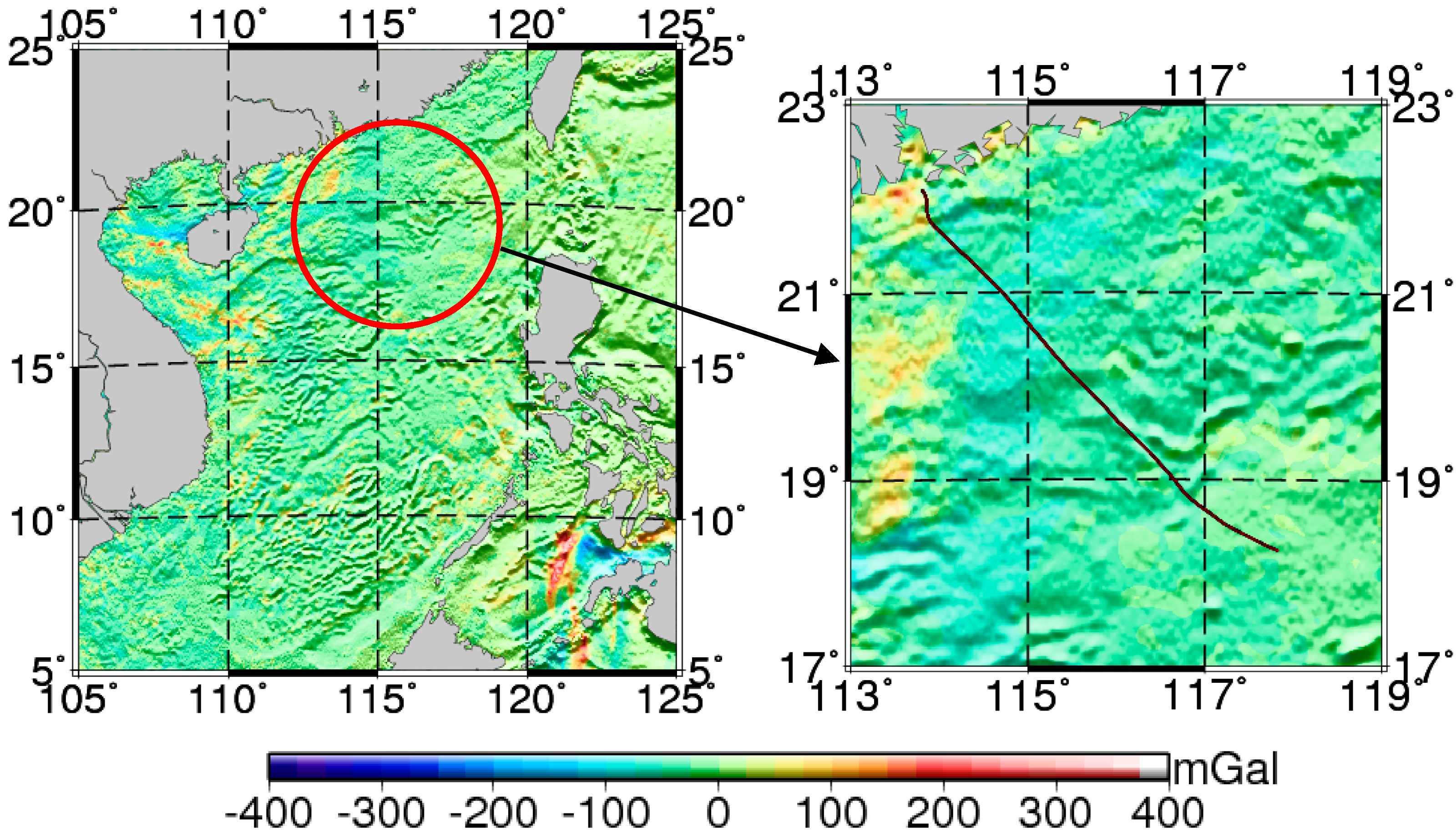
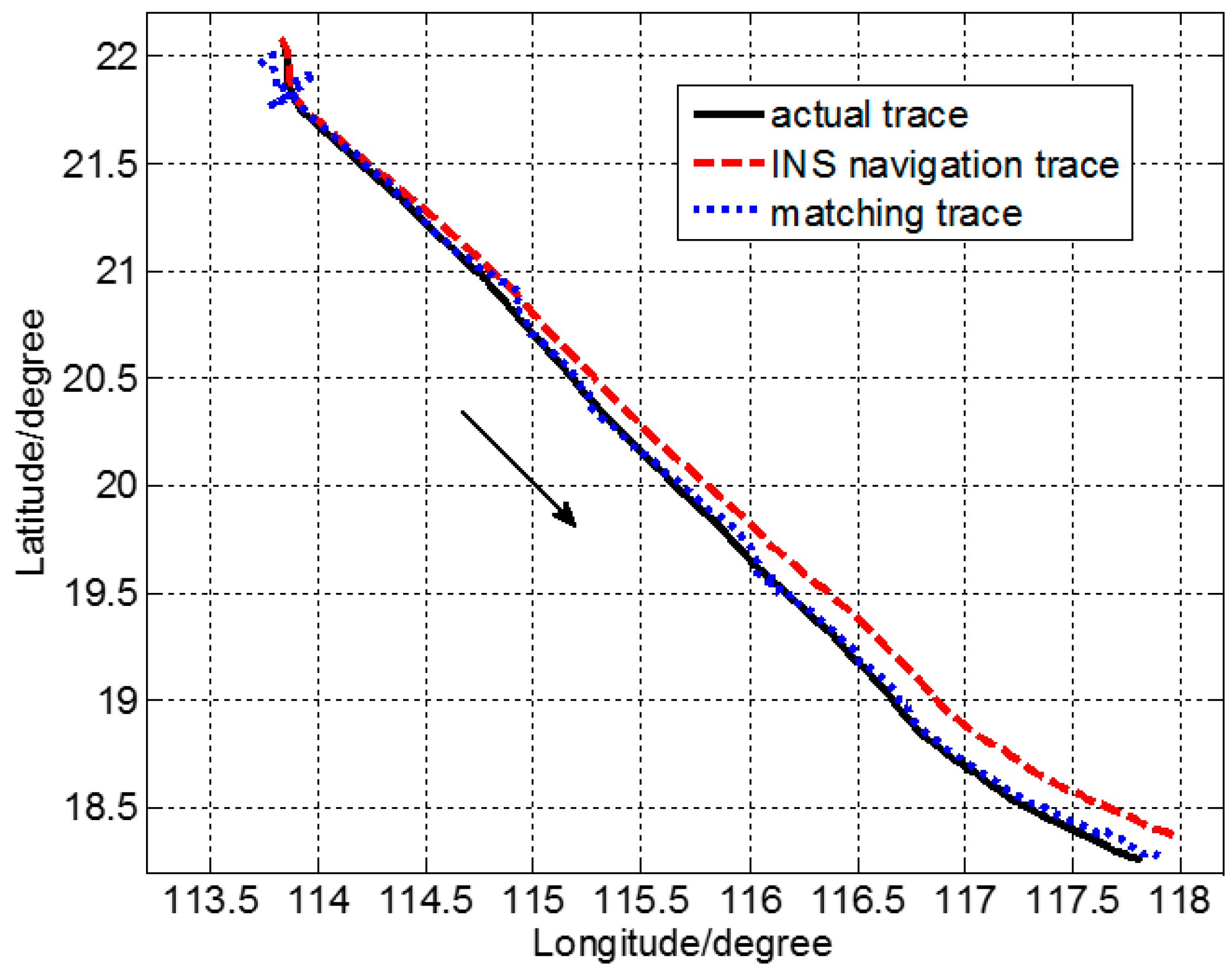
In this work, the data used in the ocean experiment were measured in the South China Sea during an exploration mission. These contained gravity data were measured using a Lacoste marine gravimeter and GPS location information along the route.
Figure 2 shows the location of the ship-measured gravity area and its corresponding route. The total length of the route was ~340 n miles. The global marine gravity anomaly model grav.img.24.1 [
31] was used for the marine gravity reference map. The reference map was constructed by the Scripps Institution of Oceanography (La Jolla, CA, USA) and had a grid resolution of 1′ × 1′. Compared to the ship-measured gravity, its overall accuracy was 3–8 mGal [
32,
33].
The location accuracy of gravity matching was closely related to the variation characteristics of the route gravity anomaly and the degree of fit between the reference map and the gravimeter observation data. For the measured gravity data
(see
in Equation (1)) from the ship route, the mean was set to
and dispersion to
, as shown in Equations (7) and (8).
Table 1 shows the preliminary results of the statistical characteristics of the measured gravity anomalies
.
was 8.5 mGal and dispersion
was 13.3 mGal. The
value of the measured gravity anomalies indicated the fluctuation (or magnitude of variation) of the gravity anomaly along the route. The greater the dispersion was, the more prominent were the gravity characteristics. The location of the expedition ship was given by GPS. Correspondingly, gravity anomalies (see
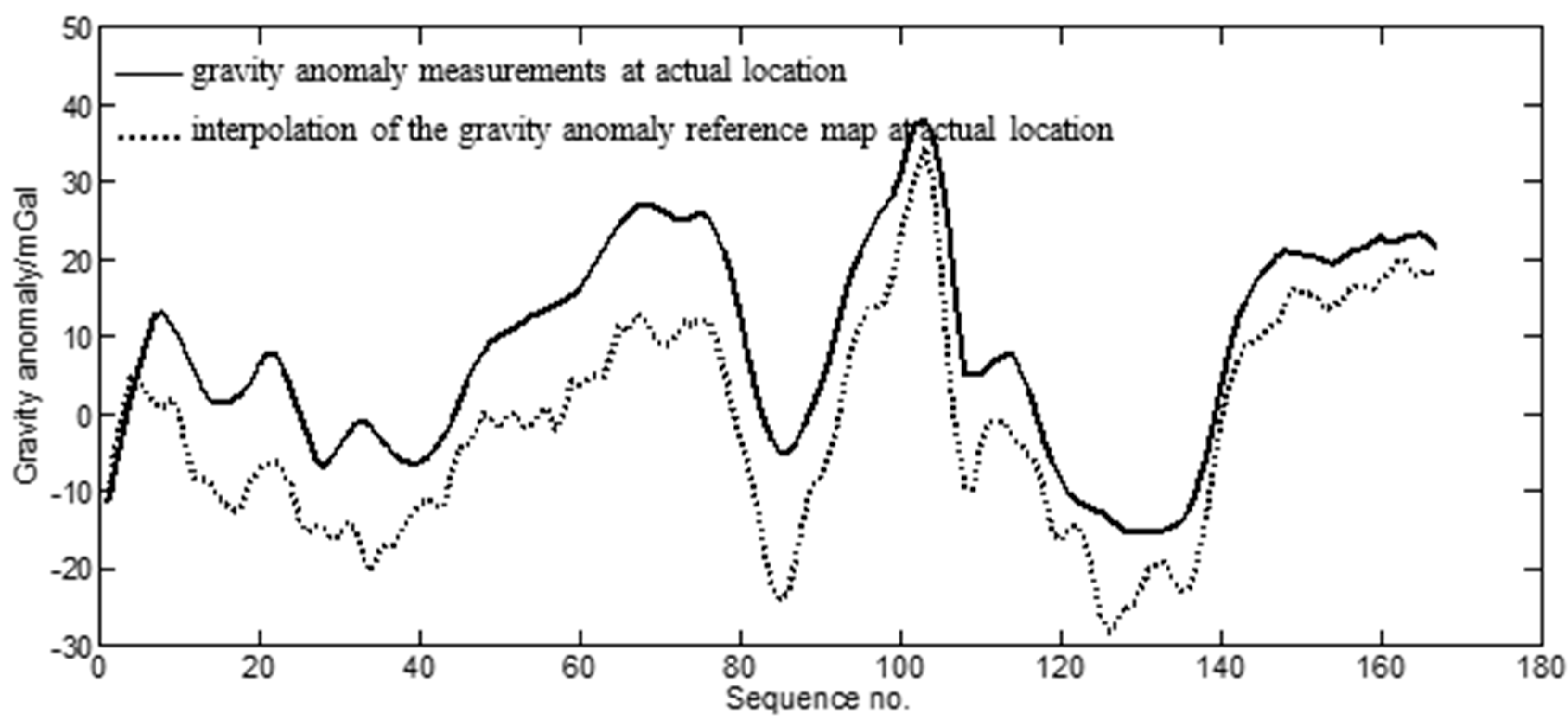
in Equation (1)) along the route were obtained by an interpolation of the gravity anomaly reference map according to the GPS location. The gravimeter-measured data along the route and those of the above interpolation were qualitatively compared, as shown in
Figure 3.
The sequence of gravity difference between the gravimeter-measured gravity anomaly along the route and the interpolation of the gravity anomaly reference map at the corresponding locations was defined by
(
). The degree of fit between the two was
, as shown by the following:
The statistical characteristics of the aforementioned difference are shown in
Table 2. According to this table, there was a 10.3-mGal systematic difference and a 4.3-mGal standard deviation between the measured gravity anomaly and the interpolated gravity anomaly at the corresponding locations on the reference map.
represents the degree of fit between the measured gravity anomaly and the gravity anomaly at the corresponding location of the reference map.
mGal, including the 10.3-mGal systematic difference and the 4.3-mGal standard deviation. As shown in
Figure 3 and
Table 2, the overall trend and characteristics were reasonably consistent between the two datasets, despite a substantial systematic difference.


