
Electromagnetic Field Assessment as a Smart City Service: The SmartSantander Use-Case


Abstract
:1. Introduction
2. Preliminaries
2.1. The LEXNET Exposure Index
- is the number of considered periods, for instance day or night.
- corresponds to the amount of different population categories in the area.
- indicates the different Radio Access Technologies (RATs) used by the end-users.
- accounts for the number of environments, such as urban, sub-urban or rural.
- represents the number of different usage profiles [5], which consider various parameters, such as the posture, traffic load, etc.
2.2. Related Work
3. EMF Testbed
3.1. SmartSantander
- IoT node: This is the entity that actually performs data acquisition. Most of them are fully integrated within a repeater, which provides the required communication capabilities, while others are deployed standalone and connect to repeaters by means of proprietary communications, which usually require wireless transmissions (for instance, ferro-magnetic sensors that are buried and provide smart-parking information).
- Repeaters: They provide the first communication level, creating a multihop capillary network that gathers the information provided by the sensing devices. The repeaters are usually deployed on walls or lampposts, and they all create a multi-hop network, based on the 802.15.4 technology. All repeaters are grouped into 25 clusters, yielding a star topology.
- Gateways: They receive the information from the repeaters and connect the capillary network with the SmartSantander backbone, where the information is stored and processed.
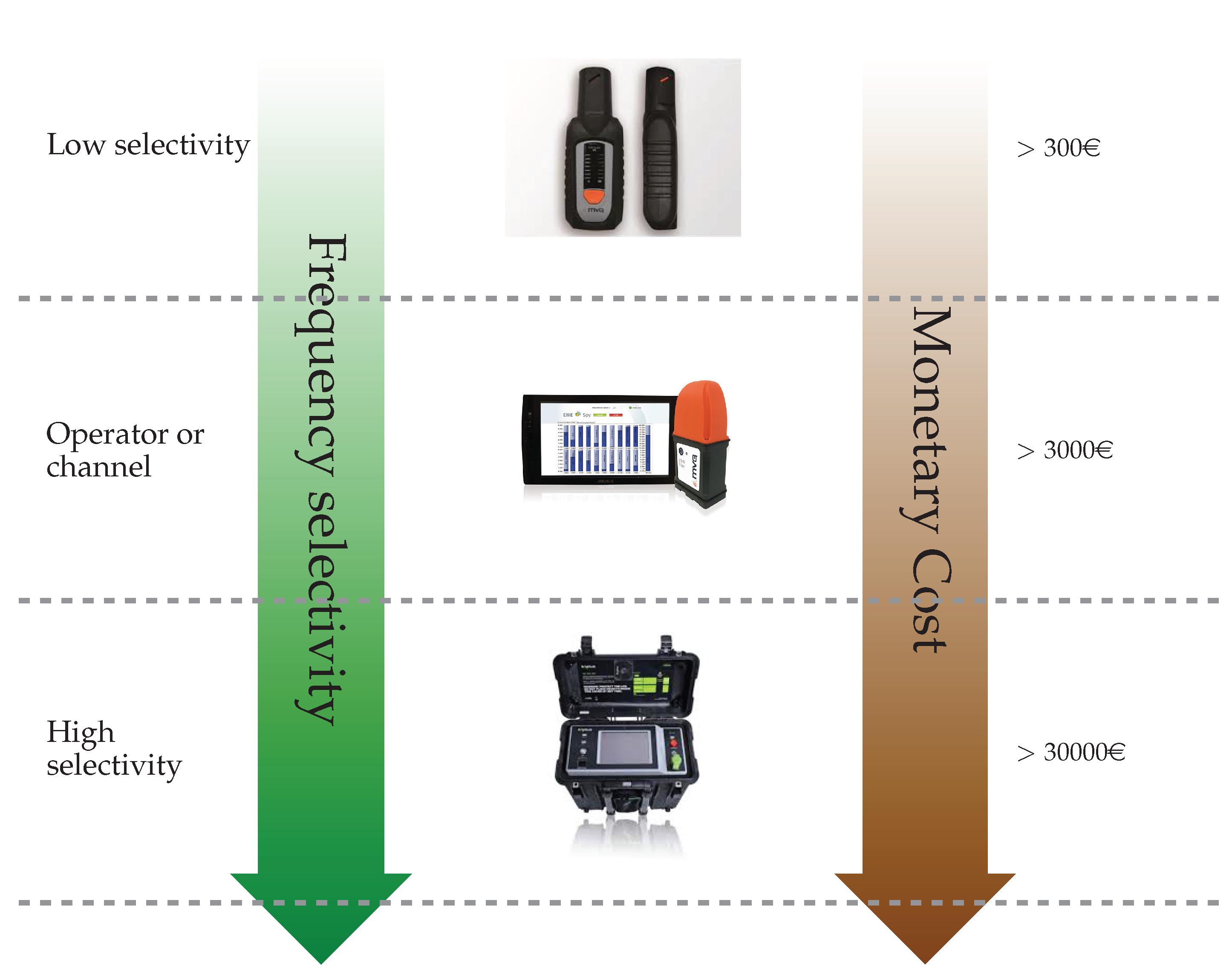
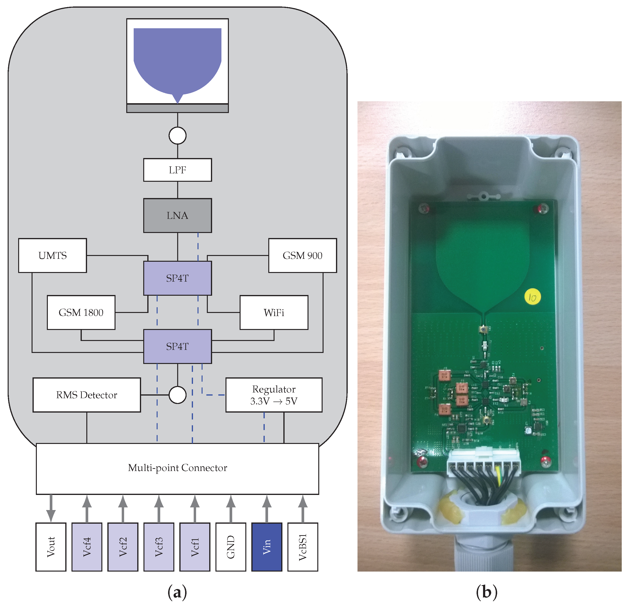
3.2. Low Complexity Dosimeter
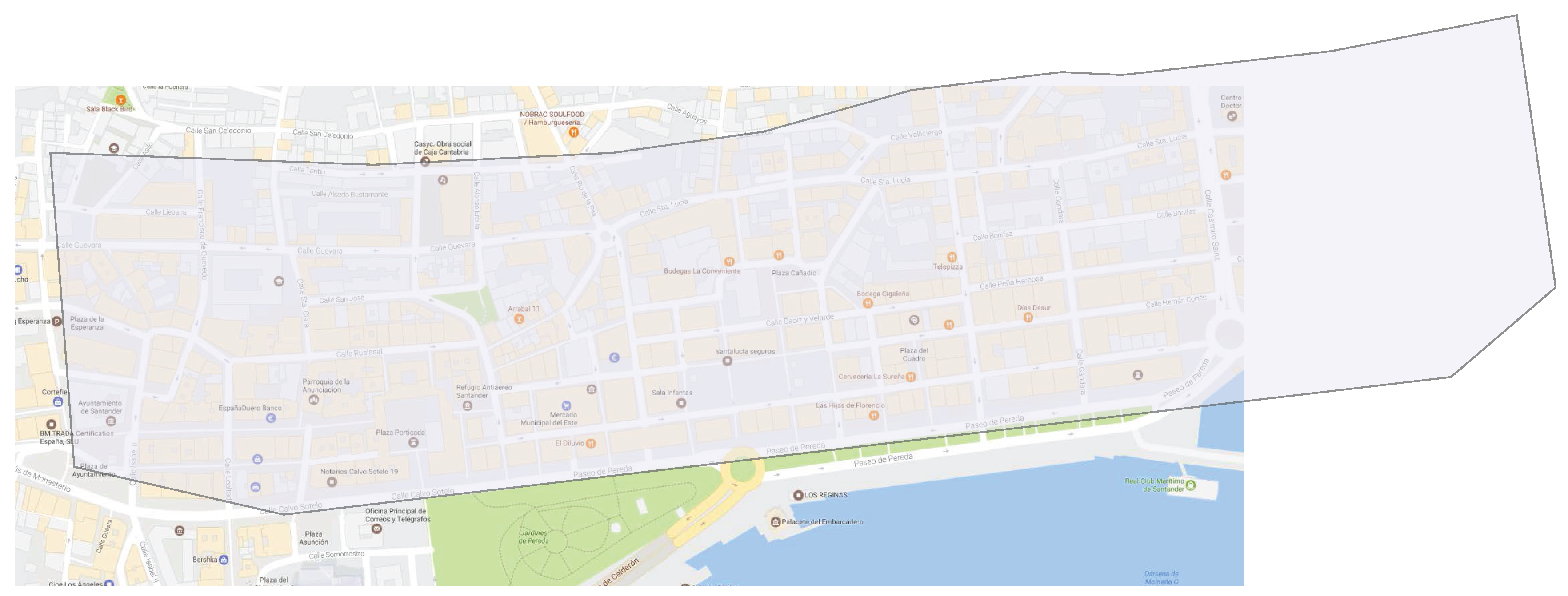
3.3. Scenario Description and Deployment Methodology
3.4. Web Portal
4. EMF Exposure Evaluation
4.1. EI Computation Methodology
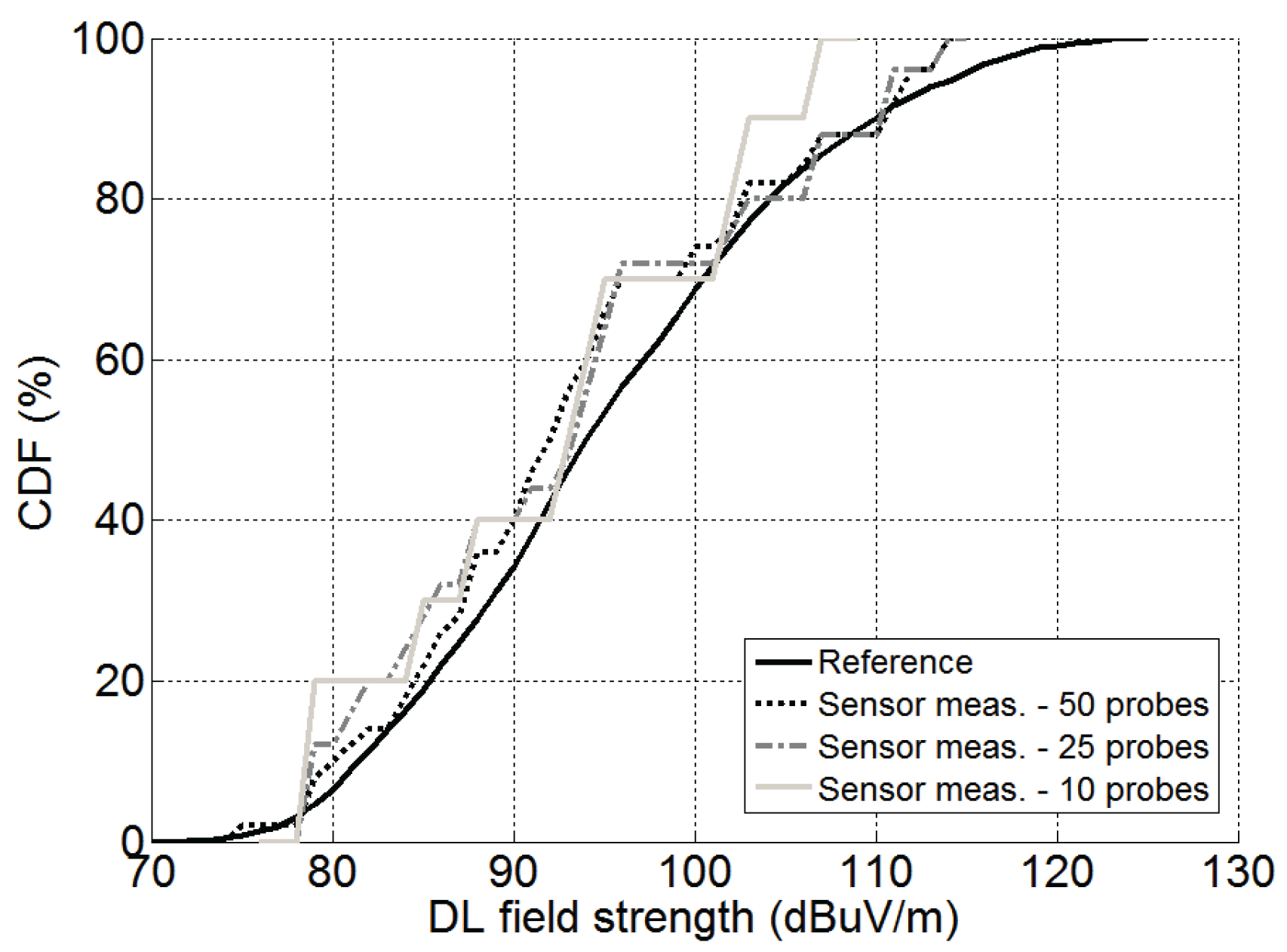
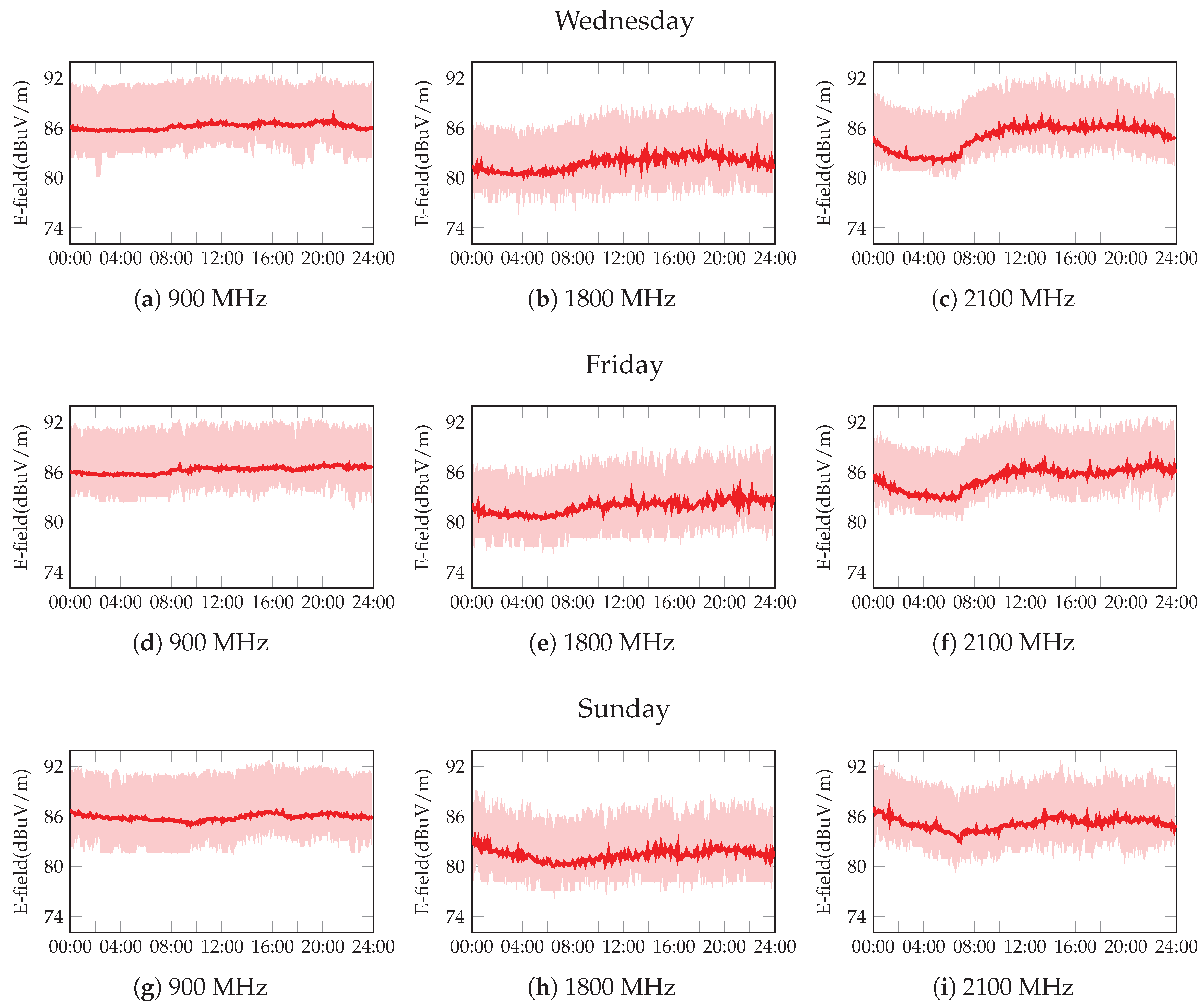
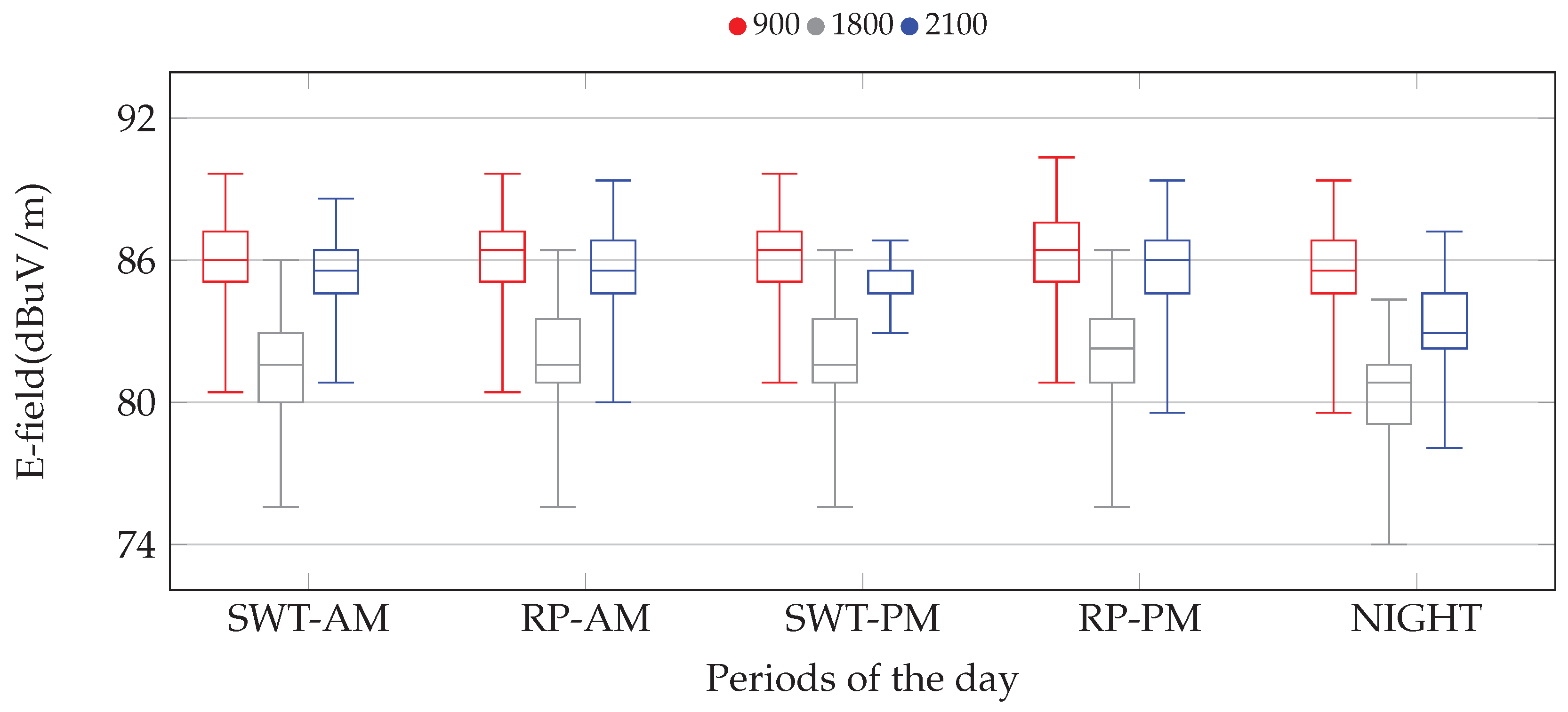
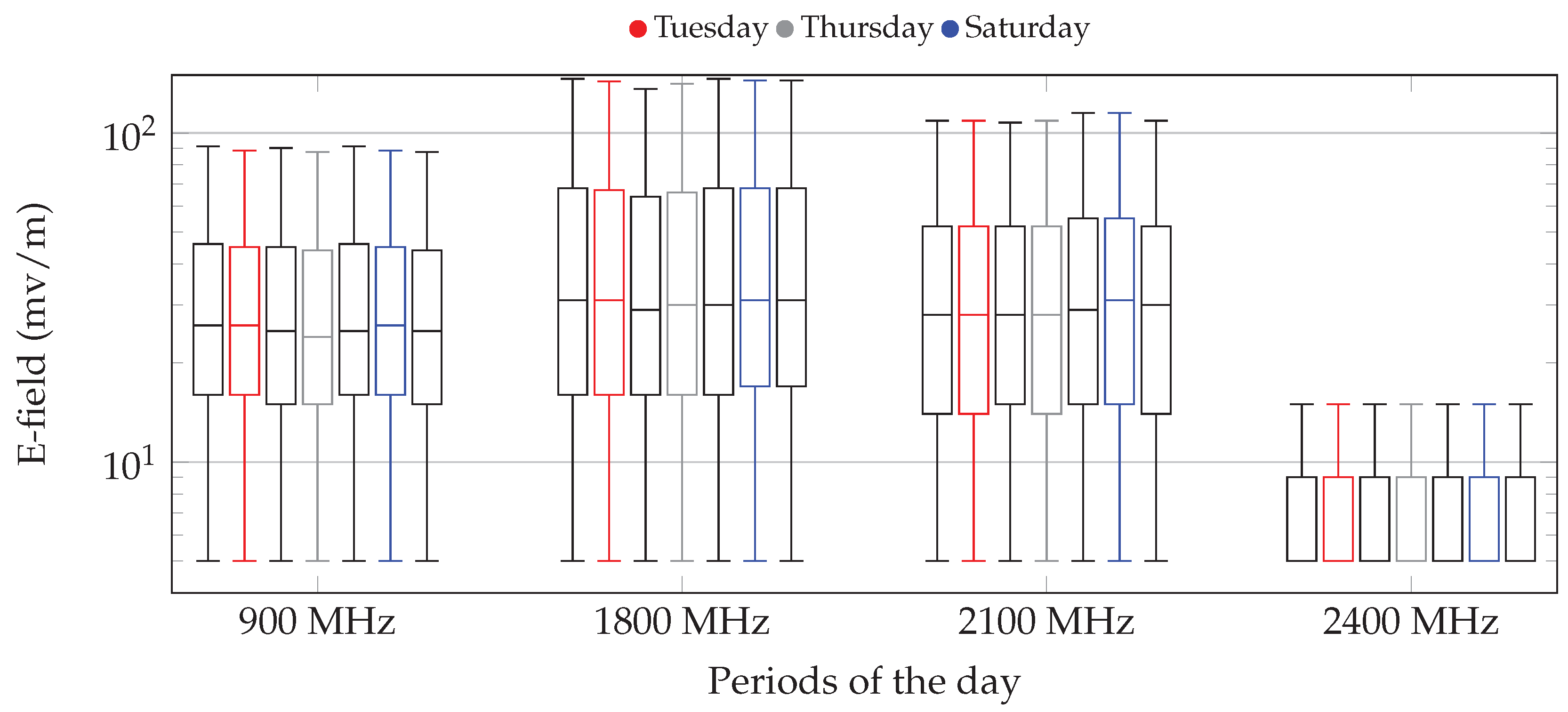
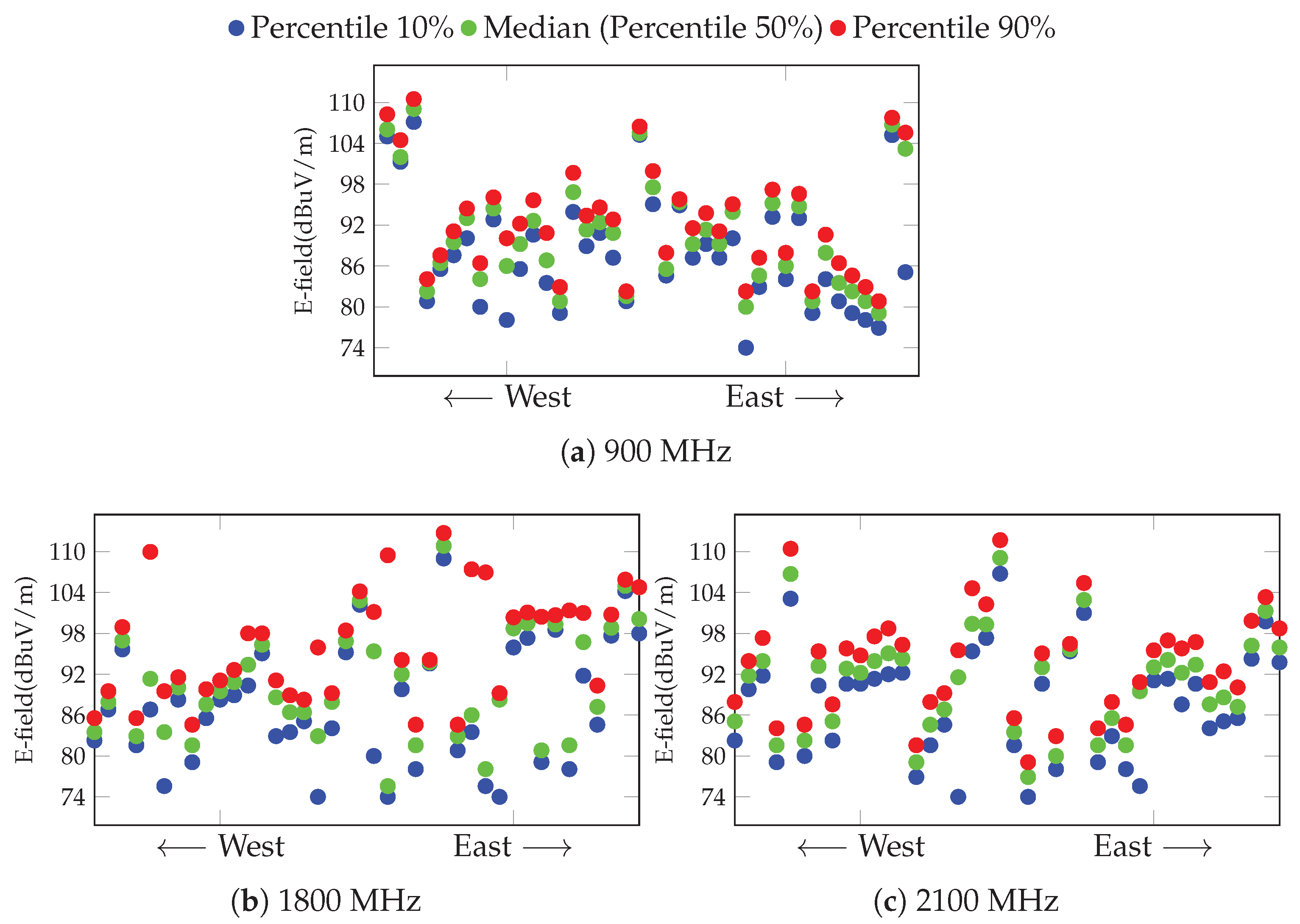
4.2. E-Field Characterization and Exposure Index
- Standard Working Time (SWT): comprises the time periods in the ranges 9:00–13:00 (a.m.) and 16:00–19:00 (p.m.)
- Rest Period (RP): is assumed to be in the ranges 14:00–16:00 (a.m.) and 19:00–22:00 (p.m.)
- Night: comprises the time interval when communications are less likely, comprising from 23:00 (p.m.) to 7:00 (a.m.)
5. Conclusions
Acknowledgments
Author Contributions
Conflicts of Interest
Abbreviations
| EMF | Electromagnetic Fields |
| LEXNET | Low-EMF Exposure Networks |
| QoE | Quality of Experience |
| EI | Exposure Index |
| IoT | Internet of Things |
| SAR | Specific Absorption Rate |
| RAT | Radio Access Technology |
| AAA | Authentication, Authorization and Accounting |
| RF | Radio Frequency |
| CDF | Cumulative Distribution Function |
| ISM | Industrial, Scientific and Medical |
| LTE | Long Term Evolution |
| PCB | Printed Circuit Board |
| RMSE | Root Mean Square Error |
| GSM | Global System for Mobile communications |
| WBSAR | Whole averaged Body SAR |
| ICT | Information and Communication Technology |
| SWT | Standard Working Time |
| RP | Rest Period |
| IQR | Interquartile Range |
References
- CISCO. Cisco Visual Networking Index: Global Mobile Data Traffic Forecast Update, 2016–2021 White Paper. Available online: http://www.cisco.com/c/en/us/solutions/collateral/service-provider/visual-networking-index-vni/mobile-white-paper-c11-520862.html (accessed on 26 May 2017).
- Tesanovic, M.; Conil, E.; Domenico, A.D.; Aguero, R.; Freudenstein, F.; Correia, L.M.; Bories, S.; Martens, L.; Wiedemann, P.M.; Wiart, J. The LEXNET project: Wireless networks and EMF: Paving the way for low-EMF networks of the future. IEEE Veh. Technol. Mag. 2014, 9, 20–28. [Google Scholar]
- Sanchez, L.; Muñoz, L.; Galache, J.A.; Sotres, P.; Santana, J.R.; Gutierrez, V.; Ramdhany, R.; Gluhak, A.; Krco, S.; Theodoridis, E.; et al. SmartSantander: IoT experimentation over a smart city testbed. Comput. Netw. 2014, 61, 217–238. [Google Scholar] [CrossRef]
- Varsier, N.; Plets, D.; Corre, Y.; Vermeeren, G.; Joseph, W.; Aerts, S.; Martens, L.; Wiart, J. A novel method to assess human population exposure induced by a wireless cellular network. Bioelectromagnetics 2015, 36, 451–463. [Google Scholar] [CrossRef] [PubMed]
- Varsier, N.; Corre, Y.; Oliveira, C.; Vermeeren, G.; Koprivica, M.; Kocan, E.; Wiedemann, P. Deliverable D2.8 Global Wireless Exposure Metric Definition. Available online: http://www.lexnet.fr/fileadmin/user/DeliverablesP2/LEXNETWP2D26Globalwirelessexposuremetricdef-V4.pdf (accessed on 26 May 2017).
- Governança Radioeléctrica. Available online: http://governancaradioelectrica.gencat.cat/web/guest/visor (accessed on 15 May 2015).
- HERMES: Project for Systematic Measurements of the Electromagnetic Radiation. Available online: http://hermes.physics.auth.gr/en/elearn (accessed on 26 May 2017).
- Oliveira, C.; Sabastiao, D.; Carpinteiro, G.; Correia, L.M.; Fernandes, C.A.; Serralha, A.; Marques, N. The moniT project: Electromagnetic radiation exposure assessment in mobile communications. IEEE Antennas Propag. Mag. 2007, 49, 44–53. [Google Scholar] [CrossRef]
- Djuric, N.; Bjelica, J.; Kljajic, D.; Milutinov, M.; Kasas-Lazetic, K.; Antic, D. The SEMONT continuous monitoring and exposure assessment for the low-frequency EMF. In Proceedings of the 2016 IEEE International Conference on Emerging Technologies and Innovative Business Practices for the Transformation of Societies (EmergiTech), Mauritius, Republic of Mauritius, 3–6 August 2016; pp. 50–55. [Google Scholar]
- Siris, V.A.; Tragos, E.Z.; Petroulakis, N.E. Experiences with a metropolitan multiradio wireless mesh network: Design, performance, and application. IEEE Commun. Mag. 2012, 50, 128–136. [Google Scholar] [CrossRef]
- LEXNET-Santander EMF Sensor Network. Available online: http://mu.tlmat.unican.es:5000/lexnet/dmapsantander.html (accessed on 15 May 2017).
- SmartSantander Maps. Available online: http://maps.smartsantander.eu/ (accessed on 15 May 2017).
- Diez, L.F.; Anwar, S.M.; de Lope, L.R.; Hennaff, M.L.; Toutain, Y.; Agüero, R. Design and integration of a low-complexity dosimeter into the smart city for EMF assessment. In Proceedings of the 2014 European Conference onNetworks and Communications (EuCNC), Bologna, Italy, 23–26 June 2014; pp. 1–5. [Google Scholar]
- Sarrebourse, T.; de Lope, L.R.; Hadjem, A.; Diez, L.F.; Anwar, S.M.; Agüero, R.; Toulain, Y.; Wian, J. Towards EMF exposure assessment over real cellular networks: An experimental study based on complementary tools. In Proceedings of the 2014 11th International Symposium on Wireless Communications Systems (ISWCS), Barcelona, Spain, 26–29 August 2014; pp. 786–790. [Google Scholar]
- Neubauer, G.; Röösli, M.; Feychting, M.; Hamnerius, Y.; Kheifets, L.; Kuster, N.; Ruiz, I.; Schüz, J.; Überbacher, R.; Wiart, J. Study on the Feasibility of Epidemiological Studies on Health Effects of Mobile Telephone Base Stations. Available online: http://www.who.int/peh-emf/meetings/archive/neubauerbsw.pdf (accessed on 26 May 2015).
- Viel, J.F.; Cardis, E.; Moissonnier, M.; Seze, R.; Hours, M. Radiofrequency exposure in the French general population: Band, time, location and activity variability. Environ. Int. J. 2009, 35, 1150–1154. [Google Scholar] [CrossRef] [PubMed]
- Project, E. Report on the Level of Exposure (Frequency Patterns and Modulation) in the European Union—Part 1: Radiofrequency (RF) Radiation. Available online: http://efhran.polimi.it/docs/D4_Report%20on%20the%20level%20of%20exposure%20in%20the%20European%20Union_Oct2010.pdf (accessed on 26 May 2017).
- Diez, L.; de Lope, L.R.; Agüero, R.; Corre, Y.; Stéphan, J.; Siradel, M.B.; Aerts, S.; Vermeeren, G.; Martens, L.; Joseph, W. Optimal dosimeter deployment into a smart city IoT platform for wideband EMF exposure assessment. In Proceedings of the 2015 European Conference on Networks and Communications (EuCNC), Paris, France, 29 June–2 July 2015; pp. 528–532. [Google Scholar]
- SIRADEL. Volcano Propagation Model. Available online: https://www.siradel.com/software/connectivity/volcano-software/ (accessed on 15 May 2017).
- Corre, Y.; Lostanlen, Y. Three-Dimensional Urban EM Wave Propagation Model for Radio Network Planning and Optimization Over Large Areas. IEEE Trans. Veh. Technol. 2009, 58, 3112–3123. [Google Scholar] [CrossRef]
- Hirata, A.; Fujiwara, O.; Nagaoka, T.; Watanabe, S. Estimation of whole-body average SAR in human models due to plane-wave exposure at resonance frequency. IEEE Trans. Electromagn. Compat. 2010, 52, 41–48. [Google Scholar] [CrossRef]
- Corre, Y.; Bories, S.; Wilson, M.; Vermeeren, G.; Vermeeren, P.; Zimmermann, P.; Lalam, M.; Anwar, S.; Stéphan, J.; Fernández, Y.; et al. Deliverable D6.2 Report on Validation, Part-A. Available online: http://cordis.europa.eu/docs/projects/cnect/3/318273/080/deliverables/001-LEXNETWP6D62ReportonvalidationPartAAres20155347928.pdf (accessed on 15 May 2017).


| Typical Application | 3GPP Band | Freq. Band (MHz) |
|---|---|---|
| GSM 900 downlink | 8 | |
| GSM 1800 downlink | 3 | |
| UMTSdownlink | 1 | |
| WiFi GHz | – |
| 50 Probes | 25 Probes | 10 Probes | |||
|---|---|---|---|---|---|
| Mean Bias (dB) | RMSE (dB) | Mean Bias (dB) | RMSE (dB) | Mean Bias (dB) | RMSE (dB) |
| Parameter | Values |
|---|---|
| Time periods | Day, Night |
| Population segments | Child (<15), Young (15–29), Adult (30–59), Senior (>59) |
| Traffic load | None, Light, Moderate, Heavy |
| Environment | Outdoor, Indoor, Commuting |
| RAT | 2G, 3G, 4G, WiFi |
| Technology | Factor | Children (13.9%) | Young (32.8%) | Adults (28.2%) | Seniors (15.1%) |
|---|---|---|---|---|---|
| Urban 2G | |||||
| Urban 3G | |||||
| Urban 4G | |||||
| WiFi | |||||
| Band (MHz) | 900 | 1800 | 2100 | 2400 |
| Mono-Axial to Isotropic | ||||
| Installation |
© 2017 by the authors. Licensee MDPI, Basel, Switzerland. This article is an open access article distributed under the terms and conditions of the Creative Commons Attribution (CC BY) license (http://creativecommons.org/licenses/by/4.0/).
Share and Cite
Diez, L.; Agüero, R.; Muñoz, L. Electromagnetic Field Assessment as a Smart City Service: The SmartSantander Use-Case. Sensors 2017, 17, 1250. https://doi.org/10.3390/s17061250
Diez L, Agüero R, Muñoz L. Electromagnetic Field Assessment as a Smart City Service: The SmartSantander Use-Case. Sensors. 2017; 17(6):1250. https://doi.org/10.3390/s17061250
Chicago/Turabian StyleDiez, Luis, Ramón Agüero, and Luis Muñoz. 2017. "Electromagnetic Field Assessment as a Smart City Service: The SmartSantander Use-Case" Sensors 17, no. 6: 1250. https://doi.org/10.3390/s17061250
APA StyleDiez, L., Agüero, R., & Muñoz, L. (2017). Electromagnetic Field Assessment as a Smart City Service: The SmartSantander Use-Case. Sensors, 17(6), 1250. https://doi.org/10.3390/s17061250