1. Introduction
In GNSS data processing, in order to avoid the rank defect issue, slant tropospheric delays along the signal paths between visible satellites and the receiver are usually mapped into the zenith direction (i.e., zenith total delay or ZTD) with a mapping function. ZTD can be divided into zenith hydrostatic delay (ZHD) and zenith non-hydrostatic delay which is always named as zenith wet delay (ZWD). ZHD, which accounts for about 90% of the ZTD, can be precisely calculated on the bases of models given the observed meteorological parameters. ZWD or the correction to
a priori ZWD which will assimilate ZTD residual errors, however, usually needs to be estimated in the data processing because of the complex variations of water vapor in both time and space. There are some empirical tropospheric delay estimation models, among which Hopfield model [
1] and Saastamoinen model [
2] are most commonly used. These two models can provide
a priori ZTD with accuracies of decimeters to sub-decimeters when precise meteorological parameters are available.
Great efforts have also been made to develop new
a priori models with good performances even without precise meteorological measurements, such as the UNB models which were initially developed for users of the Wide Area Augmentation System (WAAS). In North America, the bias of ZTD derived from UNB3 is 2.0 cm and decreases to
0.5 cm for UNB3m [
3,
4]. The deviations of ZTD derived from UNB3m, however, can reach 6.1 cm in high altitude regions [
5]. The EGNOS model, which is a simplified version of UNB3, can provide ZTD with equivalent accuracy compared to the meteorological-parameter-based Hopfield or Saastamoinen model [
6]. Li et al. developed a new global tropospheric zenith delay model (IGGtrop) based on the NCEP reanalysis data. According to their assessment using 125 International GNSS Service (IGS) stations, the mean bias and Root Mean Square (RMS) of ZTD are about 0.8 and 4.0 cm, respectively [
7,
8]. Yao et al. analyzed the temporal and spatial variations of ZTD based on Global Geodetic Observing System (GGOS) atmosphere data and built the GZTD model using spherical harmonic function. Compared to IGGtrop, GZTD has equivalent accuracies but less model parameters [
9].
A wide range of mapping functions has also been developed in the past. There are mainly two kinds of mapping functions. The first one is the so-called empirical mapping function which only needs the epoch time and stations approximate coordinates as inputs, such as the Niell Mapping Function (NMF) [
10], the Global Mapping Function (GMF) [
11] and mapping functions derived from Global Pressure and Temperature 2 (GPT2/GPT2w) [
12,
13]. These mapping functions were developed based on historical radiosondes or reanalysis products, which do not need external data in geodetic data processing. The second kind of mapping functions, such as Isobaric Mapping Functions (IMF) [
14] and Vienna Mapping Functions (VMF1) [
15], are derived from the operational analysis fields of numerical weather models at the epoch of the observations. They are theoretically more accurate than empirical mapping functions, but they rely on external data source.
Due to the strong correlation between ZTD and the vertical position, Precise Point Positioning (PPP) processing usually needs several tens of minutes to separate these two parameters for convergence, which significantly limits its real-time applications. The convergence time is much longer for users only using Chinese BeiDou Navigation Satellite System (BDS) due to the current satellite constellation, namely most of the satellites are geostationary satellites (GEO) and inclined geostationary satellites (IGSO) with slow changes of geometry relative to ground users. If the accurate
a priori ZTD are available, ZTD can be fixed or strongly constrained in PPP processing and the convergence can be efficiently accelerated [
16,
17]. However, the current
a priori ZTD models mentioned above can only provide ZTD with accuracy not better than 4 cm, which is not accurate enough for the real-time PPP [
18]. The Numerical Weather Prediction models (NWP) can also be used for retrieving real-time ZTD. For example, Andrei et al. evaluated the accuracy of hourly ZTD derived from the Global Data Assimilation System (GDAS) numerical weather model (NWM) [
19]. The average RMS of the GDAS NWM-derived ZTD is about 3 cm by comparing with IGS PPP ZTD at 18 IGS stations over 1.5 years. Lu et al. made comparisons of ZTD between ECMWF analysis and IGS solutions over one month and found an average RMS of about 1.5 to 2.2 cm which depends on the latitudes [
20,
21]. However, the NWP products are usually in the time resolution of several hours (e.g., typically from 1 to 6 h), which is not sufficient enough for high-rate real-time applications, especially, under some fast-changing weather conditions.
With the development of PPP-RTK technique, the precise ZTD derived from regional Continuously Operating Reference Stations (CORS) network have been used to interpolate ZTD for users, providing more accurate real-time ZTD than
a priori empirical models. Li et al. proposed the modified linear combination model (MLCM) for zero-difference tropospheric interpolation [
22]. Zhang et al. improved MLCM and addressed the spatial regression model with altitude difference constraint, with interpolated ZTD RMS of about 6~7 mm in flat areas and about 18 mm in undulate areas [
23]. However, these models are only valid for users in regions with CORS network available, which is usually at the scale of a city or a province.
In recent two years, there are also some publications focusing on wide-area real-time tropospheric product developments, such as [
24]. They utilized real-time GNSS stations and IGGtrop ZTD models to generate grid-based ZTD/ZWD products. In this study, we will present a new inverse scale height model and apply it to real-time ZTD solutions at GPS stations at a national scale of China to generate the real-time ZTD grid product for real-time PPP users. The data sources and processing strategy will be described in
Section 2, and the construction of the real-time ZTD grid product will be then depicted in
Section 3. The real-time ZTD grid product will be evaluated by comparisons with post-processing ZTD and by PPP convergence tests in
Section 4. Finally, some discussions and conclusions will be given in
Section 5.
3. Real-Time ZTD Grid Product Generation
In this section, the vertical variations of ZTD derived from ERA-Interim will be first analyzed and the inverse scale height model is determined and then applied to real-time ZTD solutions at GPS stations at a national scale over China for the generation of the real-time ZTD grid product.
3.1. Inverse Scale Height Model
Figure 1 presents the vertical profiles of ZTD derived from ERA-Interim at the nearest grid points from station BJFS, GDZJ and LHAS. These three stations locate in different areas in China with significantly different latitudes and altitudes. The ZTD profiles show exponentially or near exponentially decreasing trends with altitudes.
Similar to [
8], the exponential function for ZTD vertical variations can be expressed as:
where
ZTD0 is zenith tropospheric delay at MSL,
H is the scale height, and
h denotes the location altitude above MSL.
Equation (8) can also be modified to convert ZTD at a given height (
h1) to the required height (
h) as:
where
ZTD1 is zenith tropospheric delay at the given height
h1.
Considering the practical situations, we rarely do PPP for GPS receivers which are located vertically too far away from the ground surface. Therefore, we designed two ZTD fitting tests here. In the first test, the whole ZTD profiles (from 1000 hPa to 0.1 hPa) at each grid point were fitted using (9), while in the second test only ZTD at altitudes within 3 km from the terrain surface were used. The bias and standard deviation (STD) as well as the maximum and minimum values of fitting residuals are summarized in
Table 4. The comparisons show that in the terrain ±3 km test the fitting residuals are much smaller with STD of 0.42 cm. Therefore, in the following sections, we will only fit ZTD within 3 km from the terrain surface (surface altitude are acquired from ERA-Interim products) to build the inverse scale height (1/
H) model.
3.2. Inverse Scale Height Modeling
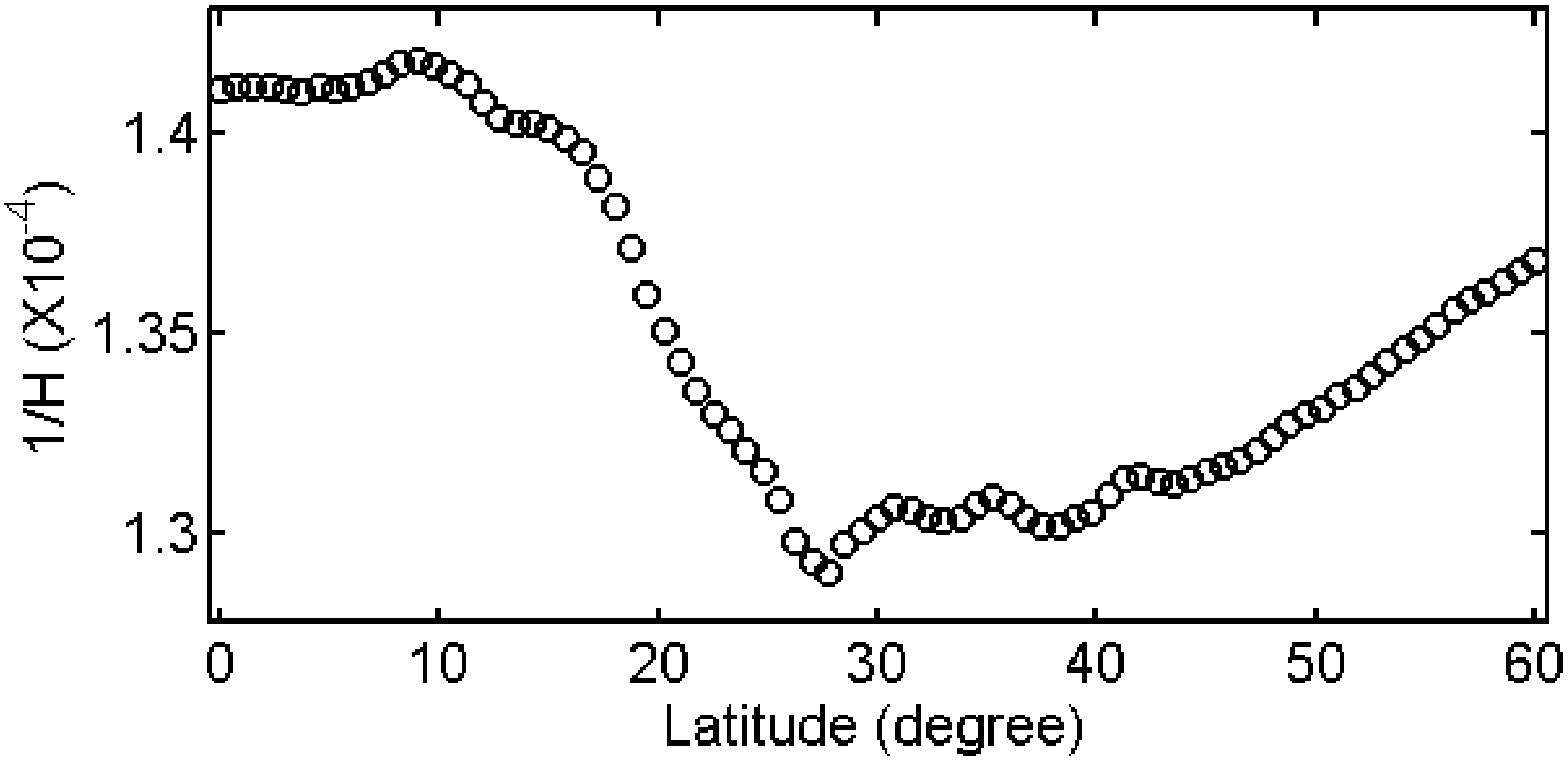
Before modeling the inverse scale height (1/H), we did a sensitivity test first to get a thumb rule regarding the relationship between 1/H and ZTD errors. ERA-Interim products for one day (1 January 2014) are used to estimate 1/H at each grid point in China. The average value of 1/H at all grid points is 1.35 × 10⁻⁴ m−1, with minimum and maximum values of 1.21 × 10⁻⁴ m−1 and 1.49 × 10⁻⁴ m−1, respectively. The average value of 1/H instead of the actual 1/H was then used in (8) to estimate ZTD at each grid point and the differences between the estimated ZTD and the actual ZTD were calculated. According to the statistics, we found a change of 1/H with 0.1 × 10⁻⁴ m−1 corresponds to about 2.8 cm in ZTD.
Figure 2 presents the distribution of mean 1/
H at different latitudes over China. The amplitude is larger than 0.1 × 10
−4 m
−1, which corresponds to about 2.8 cm ZTD according to the sensitivity test. In addition, according to our statistics, the differences of 1/
H at different longitudes in the same latitude can reach 0.2 × 10
−4 m
−1 (corresponds to 5.6 cm of ZTD). Obviously, 1/
H has considerable spatial variations, which needs to be taken into account when modeling 1/
H.
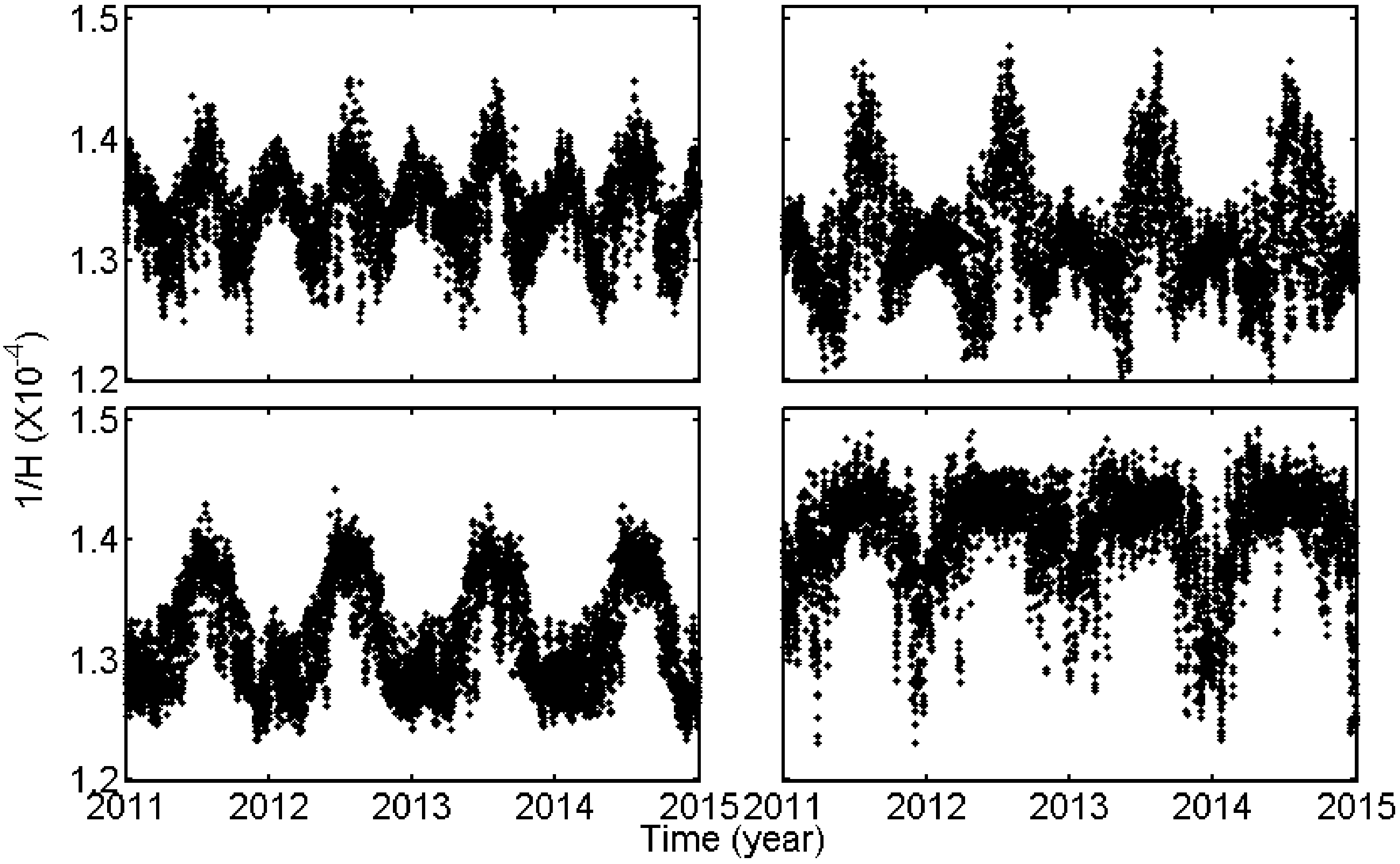
The temporal variations of 1/
H were studied on the bases of 4-year (2011~2014) time series of 1/
H. As an example, the time series of 1/
H at nearest grid points from four GPS stations (HLHG, BJFS, LHAS and GDZJ) are shown in
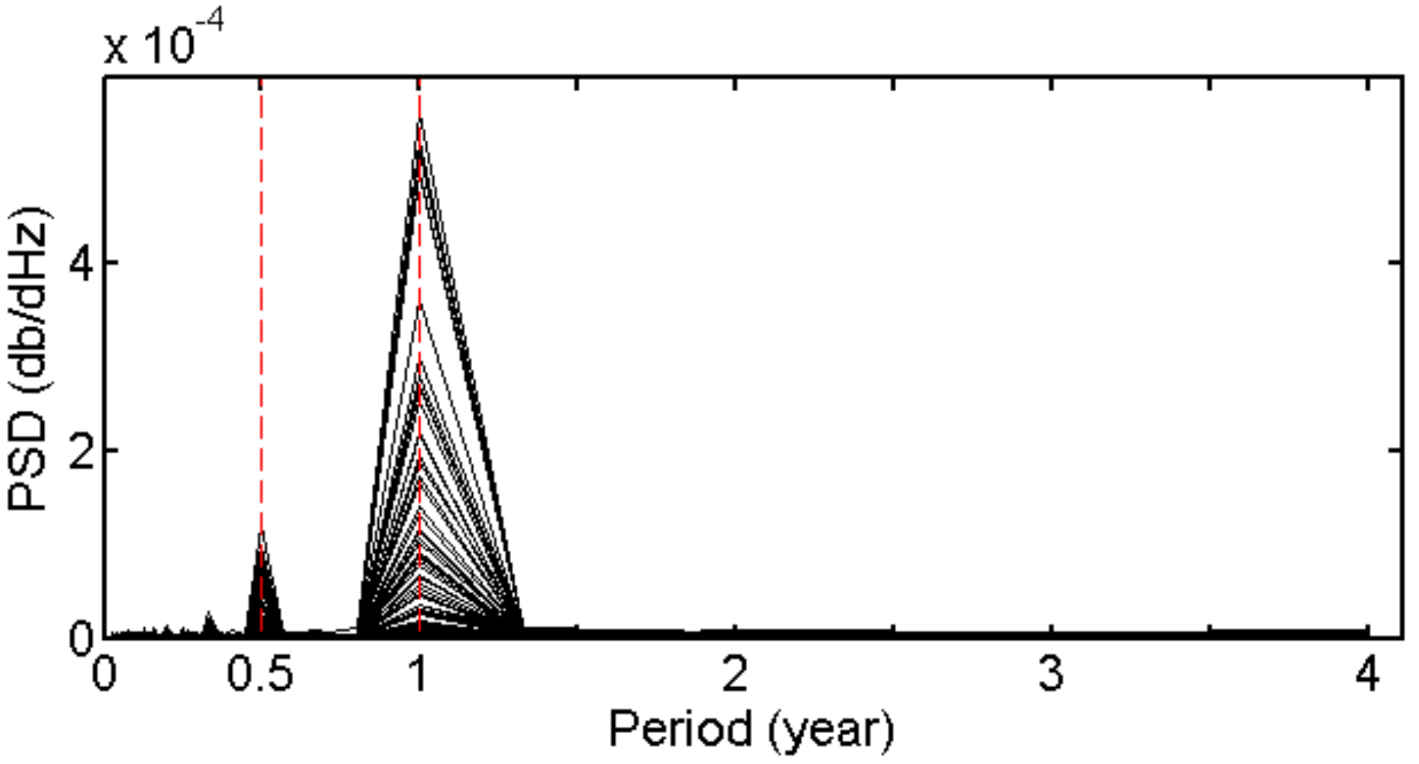
Figure 3 where we can find obvious periodical signals. The Power Spectral Density (PSD) of 1/
H time series at all grid points over China are presented in
Figure 4, where we can find the time series mainly contain annual and semi-annual periodical signals. Therefore, we used the model as expressed in (10) to fit 1/
H at each grid point:
where
a0~4 are coefficients.
Based on the above analysis, ZTD time series covering the period from 2011 to 2014 at each grid point (0.75° × 0.75° resolution) derived from ERA-Interim were used to estimate 1/H by (8). The inverse scale height time series at each grid point were then fitted by (10) to generate a coefficient (a0, a1, a2, a3, a4) table. The Mean Absolute Error (MAE) and RMS of fitting residuals are 0.03 × 10⁻⁴ m−1 and 0.039 × 10⁻⁴ m−1, corresponds to 0.84 cm and 1.09 cm of ZTD, respectively.
3.3. Real-Time ZTD Grid Product Generation Procedure
ZTD at GPS stations in CMONOC were estimated in the simulated real-time mode using PANDA package with 5 min interval. For each grid point with horizontal resolution of 0.75° × 0.75° covering the area of 10° N~60° N and 70° E~140° E, the GPS stations within 1000 km near the grid point were selected. ZTD at these GPS stations were converted from the station altitude to the grid point surface altitude using the above inverse scale height model which can be expressed as:
where the subscripts of
ci and
g denote the station and the grid point, respectively.
The inverse distance weighted (IDW) method was then applied to calculate the ZTD at the grid point as,
where
pi is the weight coefficient for each station. In order to make the product easy to use, the ZTD at the grid point surface were eventually converted to MSL using the inverse scale height model.
For users, ZTD at the nearest four grids around the user were converted from MSL to the user’s altitude by inverse scale height model and then IDW method were used for horizontal interpolation to calculate the ZTD at user’s location.
5. Discussion and Conclusions
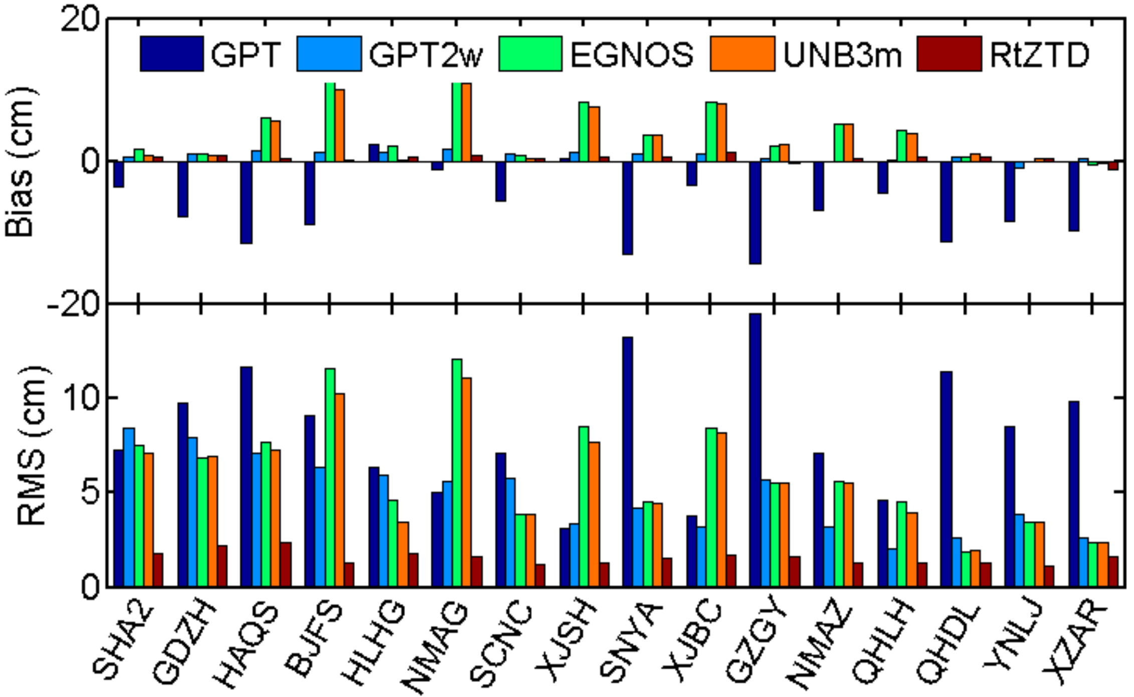
The temporal and spatial variations of ZTD with altitude over China were analyzed on the bases of the latest meteorological reanalysis products (ERA-Interim). Results show that the variations of ZTD with altitude are near exponential, and the temporal variations of exponential function coefficients at specific location mainly contain annual and semi-annual periodical signals. An inverse scale height model was then determined and applied to ZTD solutions derived from CMONOC GPS stations in simulated real-time mode to generate the ZTD grid products. Using 16 stations in CMONOC as test stations, the ZTD derived from the ZTD grid product were compared to ZTD estimated in post-processing mode and the average bias and RMS of the ZTD differences are 0.39 cm and 1.56 cm, respectively.
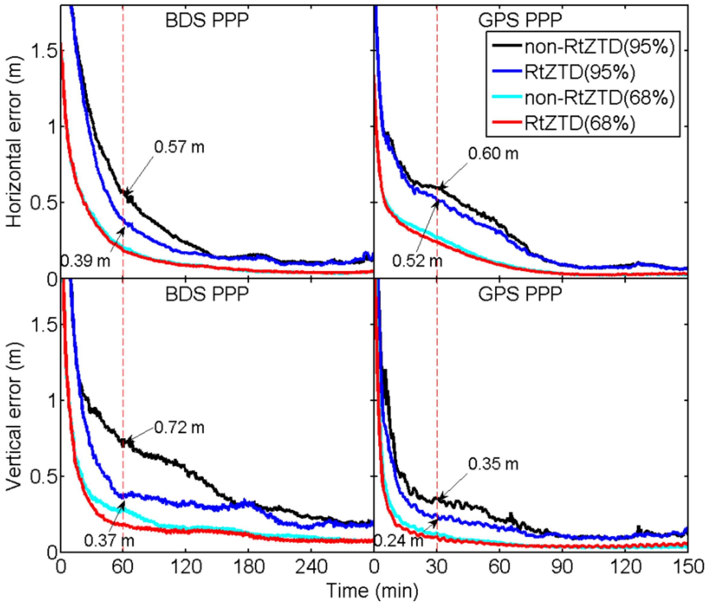
All GPS stations in CMONOC were used to generate RtZTD products in simulated real-time mode, and 95 stations with GPS and BDS observations in NBASS were taken as test stations for PPP convergence tests. Data covering one week were processed and the convergence time of PPP with and without RtZTD products used were compared. Regarding the convergence time, the thresholds for convergence were determined based on coordinate error RMS statistics, i.e., 0.4 and 0.2 m of coordinate errors for BDS- and GPS-PPP, respectively, in 95% statistics, while 0.2 and 0.1 m for BDS and GPS, respectively, in 68% statistics. The results show considerable improvements in convergence time by using RtZTD of about 32% (6%) and 65% (65%) in the horizontal and vertical components for BDS-PPP, and 29% (25%) in vertical direction for GPS PPP in 95% (68%) statistics.
The time delays, including transmission time from reference stations to the data center, data processing time and transmission time from the data center to users, are generally smaller than 10 s in current augmentation systems. For example, the total time delays in the Global Differential GPS (GDGPS) System developed by JPL are smaller than 5 s. Considering the relatively small variations of orbit and clock corrections (<1 cm) and ZTD (<1 mm) in small intervals like 10 s (variations not shown here), these time delays can be safely ignored in real-time applications. This is also the reason why in some satellite-based augmentation system services, e.g., the QZSS L6 signal, which provides centimeter level augmentation services, can broadcast orbit and clock corrections in 30 and 5 s intervals without using any prediction models, and why IGS centers can estimate ZTD as constants in 5 min intervals. Therefore, although all real-time tests in this work were carried out in the simulated mode with time delays ignored, the conclusions can provide important references to real-time applications. As more and more real-time GPS stations are available in China, we can expect better and more robust results in the near future.


