1. Introduction
Road scene simulation and modeling based on vehicle sensors are currently an important research topic in the field of intelligent transportation systems [
1,
2]. The data acquired from vehicle-mounted sensors mainly include images, laser scans, and GPS. Once acquired, road scene modeling results can be applied to the simulation of photo-realistic traffic scenes.
A key use of such simulation is for the purposes of road safety, especially with regard to unmanned vehicles. Extensive tests and evaluations need to be performed to ensure the safety and robustness of unmanned vehicles. These mainly involve the field tests and offline tests. Field tests are the most traditional way to proceed. Micky Town at Michigan State and Google’s Castle Atwater in California have both been constructed to undertake unmanned vehicle evaluation. To be effective, field tests have to be implemented on different types of roads including urban roads, rural roads and highways. However, there are a number of drawbacks to using field tests, such as limited driving space, the time and effort involved in constructing them and their significant monetary cost. As a result, offline tests have become an increasingly important complement to field-based evaluation.
Early studies using offline testing were designed around computer graphics methods. Typical applications here included Prescan from TNO (Netherland) [
3] and CarMaker from IPG (United States) [
4]. Recently, road scene modeling based on road image sequences has become popular, for instance Google Street View [
5] or Microsoft Street Slide [
6]. These systems provide users with an immersive touring experience while browsing a map. The Waymo Team at Google (California, USA) have constructed a virtual scene platform from road image sequences that can be applied to the simulation of virtual roads for billions of miles.
In this paper, we propose a new framework for road scene simulation from road image sequences. This specific application we have in mind for this framework is the offline testing of unmanned vehicles. The framework consists of two successive steps: (1) the detection of road and foreground regions’ detection; and (2) the construction of scene models. For the first step, we have developed a region detection method based on a superpixel-level random walk (RW) algorithm, which is further refined by a fast two-cycle (FTC) level set approach. For the second step, foreground and background models are constructed using scene stages. “Floor-wall” structured traffic scenes are then established.
The main contributions of this work can be summarized as follows:
The development of a novel region detection method using a superpixel RW algorithm. The superpixel features are computed using a combination of color, texture and location information. Region seeds for the RW algorithm are initialized through region-related trapezoids using an optical flow map. An FTC level set is then employed for region refinement.
The development of a new framework for constructing 3D scene models based on scene stages. The scene stages are specified according to the detected road and foreground regions. 3D scene models are then constructed on the basis of graph models of the scene stages.
The development of a new system to simulate traffic scenes. Two modes are designed for the simulation of traffic scenes: (1) an interactive touring mode, and (2) a bird’s-eye view mode. This system can form the basis of the offline testing of unmanned vehicles.
2. Related Works
The framework of this paper consists of several components, which mainly includes region detection and scene model construction. In this framework, the computation of the superpixel features is an important pre-processing step. A new RW algorithm is then proposed based on the superpixel features. The road scene models are further constructed based on the region detection results. The related works are summarized in the areas of region detection and scene model construction.
Superpixels are the mid-level processing units widely used in the computer vision community. Schick et al. [
7] convert the pixel-based segmentation into a probabilistic superpixel representation. A Markov random field (MRF) is then applied to exploit the structural information and similarities to improve the segmentation. Lu et al. [
8] specify the superpixel-level seeds using an unsupervised learning strategy. The appropriate superpixel neighbors are further localized by a GrowCut framework. However, the vanishing points in the images must be detected as a pre-processing step. Siogkas et al. [
9] propose a RW algorithm integrating spatial and temporal information for road detection. Nevertheless, this pixel-level RW algorithm has the drawback of low efficiency and slow speed. Shen et al. [
10] present an image segmentation approach using lazy random walk (LRW). The LRW algorithm with self-loop has the merits of segmenting the weak boundaries. However, this method cannot be applied to image sequences since the spatio-temporal superpixel features are not considered. The similar studies include the fixation point-based segmentation [
11], etc. Recently, the region detection methods based on convolutional neural networks (CNN) become popular. Teichmann et al. [
12] apply deep CNN to jointly reason about classification, detection and semantic segmentation based on the KITTI road dataset [
13]. The effectiveness of residual networks (ResNet) [
14] and VGG [
15] are also evaluated. However, the training of the networks is computationally expensive.
The 3D scene models can be constructed based on the region detection results. Saxena et al. [
16] propose a method to learn plane parameters using an MRF model. The location and orientation of each mesh facet can be judged to construct the 3D wireframe of the scene model. However, this method lacks a hypothesis about the scene layout, and the computation of the image features is time-consuming. Hoiem et al. [
17] apply superpixel segmentation to the input images, and then utilize a support vector machine (SVM) for superpixel clustering. Delage et al. [
18] apply a dynamic Bayesian network to automatically judge the edge pixels between the floor and wall regions for indoor images. The “floor-wall”-structured scene model is then constructed. Unfortunately, this scene model cannot be applied to the outdoor images. The Tour into the Picture (TIP) model of Horry et al. [
19] partitions an input image into regions of “left wall”, “right wall”, “back wall”, “ceiling” and “floor”. The foreground objects are assumed to stand perpendicularly to the floor plane. The main drawback of the TIP model lies in the fact that it is applicable to the curved floor conditions. Nedovic et al. [
20] introduce the typical 3D scene geometries called stages, each with a unique depth profile. The stage information serves as the first step to infer the global depth. Lou et al. [
21] propose an approach that first predicts the global image structure, and then extract the pixel-level 3D layout. However, the prediction of the scene stage label is complex and computationally expensive.
The comparison of the previous studies is shown in
Table 1, where region detection and scene construction are summarized, respectively.
The rest of the paper is organized as follows: The superpixel-level RW method and FTC refinement is presented in
Section 3. In
Section 4, the construction of road scene models is introduced. Experiments and comparisons are shown in
Section 5. Finally, we close this paper with conclusion and future works.
3. Random Walk for Region Detection at a Superpixel Level
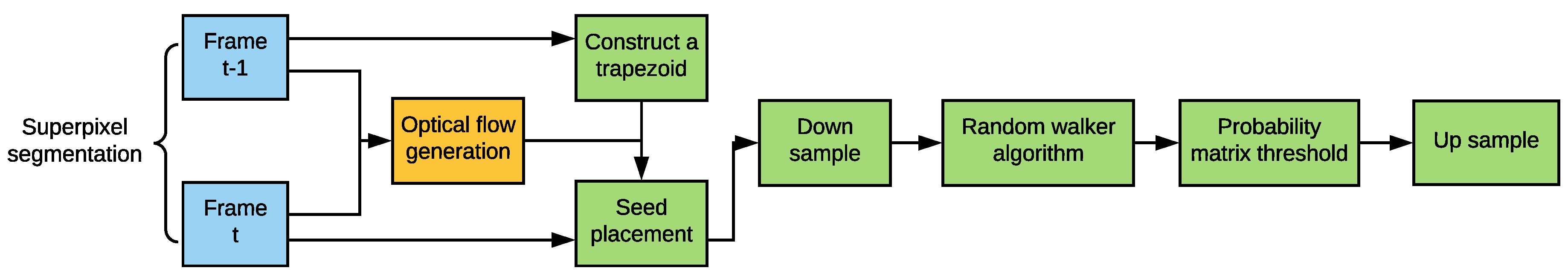
In order to reconstruct road scene models, the road and foreground regions in each frame have to be detected first of all. To do this, we use a region detection method based on an RW algorithm. The road and the foreground regions of the first frame are specified by means of user annotation. For the rest of the frames, corresponding regions are detected based on the seeds propagated from the previous frames. The detection flow diagram for an example frame
t is shown in
Figure 1.
3.1. Superpixel Segmentation
For the region detection we use superpixel segmentation, specifically adopting the Ncut method [
22], with superpixel features being extracted as the basis of the algorithm (see,
Table 2). Color, texture and location descriptors are combined to denote the superpixel features. The color descriptor mainly used the HSV and CIElab color spaces. The texture descriptor is composed of a Gabor filter and a local binary pattern (LBP). The location descriptor consists of a convex hull, a clique number, etc. These descriptors are then concatenated into an overall vector.
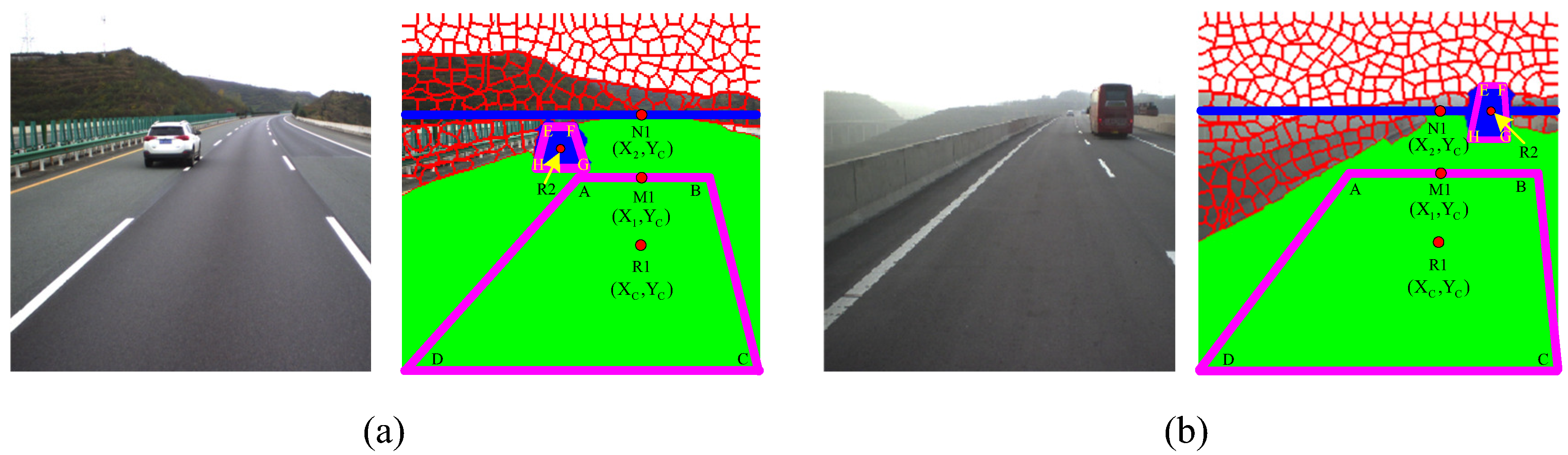
3.2. Definition of Seed Trapezoid
Seed trapezoids for the road and foreground regions are depicted in
Figure 2. If
is taken to be the center of the detected road region of frame
,
can be denoted as the upper bound, with the same vertical coordinate as the centroid. The bottom line of the trapezoid (
) is the same as frame
’s road base. The top of the trapezoid (
) is equal to the perpendicular distance for
. The seed trapezoid seed for the road region can then be specified. The trapezoid for the foreground region is defined in a similar way, as shown with regard to the placement in
Figure 2.
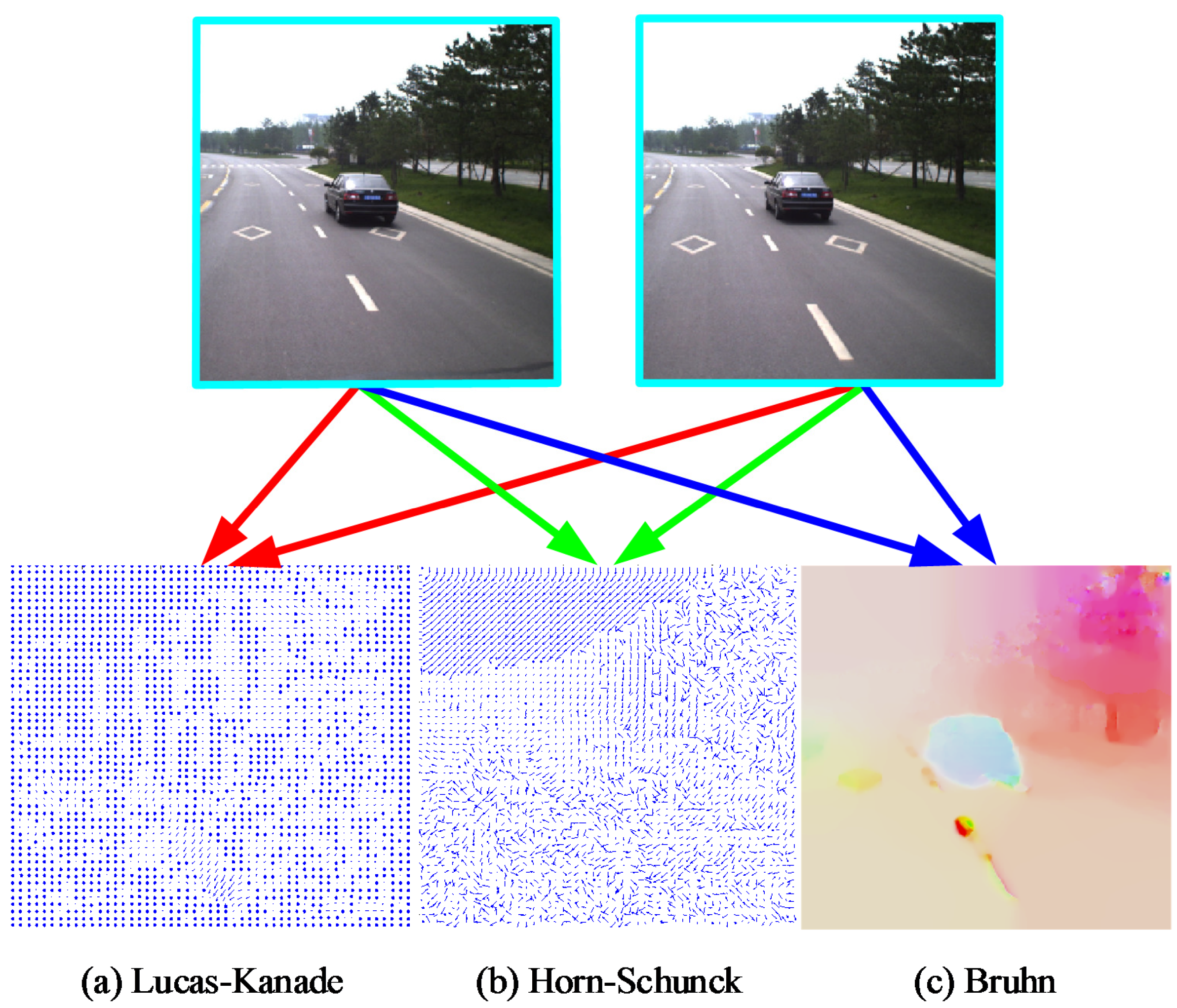
3.3. Seed Trapezoid Initialization by Optical Flow
The trapezoid of a certain frame
t is initialized in frame
using an optical flow map. Optical flow map generation is typically classified into (1) sparse optical flow and (2) dense optical flow. Sparse optical flow is computed from the local feature points in images, e.g., by using the Lucas–Kanade algorithm [
23]. Dense optical flow, however, attempts to compute the optical flow information for all of the pixels in an image, for instance, by using the Horn and Schunck [
24] approach. The Bruhn method [
25] brings together the advantages of both sparse and dense optical flows. A dense optical flow field is generated by using this method that is robust under conditions of environmental noise. A comparison of the results produced by the Lucas–Kanade, Horn–Schunck and Bruhn methods are shown in
Figure 3.
3.4. Random Walk Detection at a Superpixel Level
The superpixel-level RW detection is shown in Algorithm 1. Its basic steps are as follows:
The input image is transformed into the graph:
, where the graph nodes denote the superpixels. The weight of the edges in the graph are defined as follows:
where
and
are the features of superpixels
i and
j, while
and
denote the respective superpixel locations. The superpixel features are represented by a concatenation of the color and texture vectors:
where
denotes the color feature of the current superpixel.
denotes the texture feature, which is extracted by a Gabor filter. The image block centered at the current superpixel is used to compute the output vector of the Gabor filter. The superpixel features match those described in
Section 3.1.
A Laplacian matrix is now defined to denote the superpixel probability labels:
where
is the superpixel value indexed by
and
, and
is the degree for
on all edges
.
Next, vertices of the graph
G are partitioned into two groups: a seeded set
and an unseeded set
. These two sets satisfy the following requirements:
and
. The Laplacian matrix can now be redefined as:
where
and
are the seeded and unseeded pixels in
L and
is the decomposition result.
The Dirichlet integral is:
where
x is a function that minimizes Equation (
5) and
is an edge of the graph connecting the vertices
and
.
The decomposition of Equation (
5) can be defined as:
where
and
are the sets of regional probabilities corresponding to the unseeded and seeded superpixels. Differentiating
with respect to
yields
This equation can be solved using the method outlined in [
9], with it being considered to be a two-class segmentation problem.
3.5. Region Refinement Using an FTC Level Set
The region detection algorithm described above is effective for most conditions. However, as the computing units of the algorithm are superpixels, there is a risk that, if the superpixel features are similar in the foreground and background regions, it may fail to get accurate results. To solve this problem, a fast two-cycle (FTC) level set method can be applied that is based on pixels for region refinement. The main data structure for this method is composed of three parts: an integer array
as the level set kernel matrix, an integer array
for the speed function and two linked lists of boundary pixels to denote the foreground contours
and
. The foreground contours are initialized from the regions detected by the superpixel-level RW algorithm. In order to facilitate curve evolution of the FTC level set, the first cycle should be conducted to establish the data fidelity terms, then a second cycle should be conducted to establish the data smoothness terms. The pixels inside
are called interior pixels, and the pixels outside
are called exterior pixels. The kernel matrix can be defined as:
The speed function
is defined according to the competition terms between the foreground and background regions [
26]. The curve evolution can then be determined by using the signs of the speed function rather than by solving any partial differential equations. The speed function is as follows:
where
and
are the feature pools for the foreground and the background, respectively.
and
are the color and texture feature vectors extracted at pixel
y. After definition of the kernel matrix and speed function, the curve evolution can be implemented across two cycles. The first cycle is for the boundary pixel evolution. The second cyle is for the boundary smoothness. The functions
and
can be used for the curve evolution [
27]. The region refinement examples based on the FTC level set are shown in
Figure 4.
The region detection algorithm based on a superpixel-level RW with FTC refinement is summarized in Algorithm 1.
| Algorithm 1 Region detection based on a superpixel-level RW with FTC refinement |
- 1:
Initialize the regions and trapezoids for the frame ; - 2:
(1) Region detection based on a RW at superpixel level: - 3:
for t = 1 to M do - 4:
Compute the optical flow map between frame t and ; - 5:
Initialize region seed of frame t using the trapezoid of frame on the basis of the optical flow map; - 6:
Down-sample frame t to a lower resolution; - 7:
Implement the RW algorithm for frame t; - 8:
Implement the threshold for the probability matrix to get the detection results; - 9:
Up-sample frame t to the original resolution; - 10:
end for - 11:
(2) Region refinement based on the FTC level set: - 12:
for t = 1 to M do - 13:
Initialize and based on the RW detection results; - 14:
Define the speed function using Eq. (9); - 15:
Undertake the Fast Two-Cycle curve evolution; - 16:
Get the refined regions according to the contours; - 17:
end for
|
4. Road Scene Construction and Simulation
After detection of the road and foreground regions, the corresponding static and dynamic traffic elements can be extracted. The scene models are then constructed based on the scene stages. These form the basis of the road scene simulation process.
4.1. Scene Model Construction
In order to construct the road scene models, a graph model can be used for each image to represent the connection between the foreground and background regions:
where
N and
E represent the scene nodes and the corresponding relationships. For the
ith image,
and
are defined by:
where
,
,
, and
denote “road plane”, “left wall”, “right wall” and “back wall”, respectively.
and
are the control points of road boundaries on each side [
1].
denotes the
n foreground objects, while
are the positions of rht foreground polygons standing on the road plane.
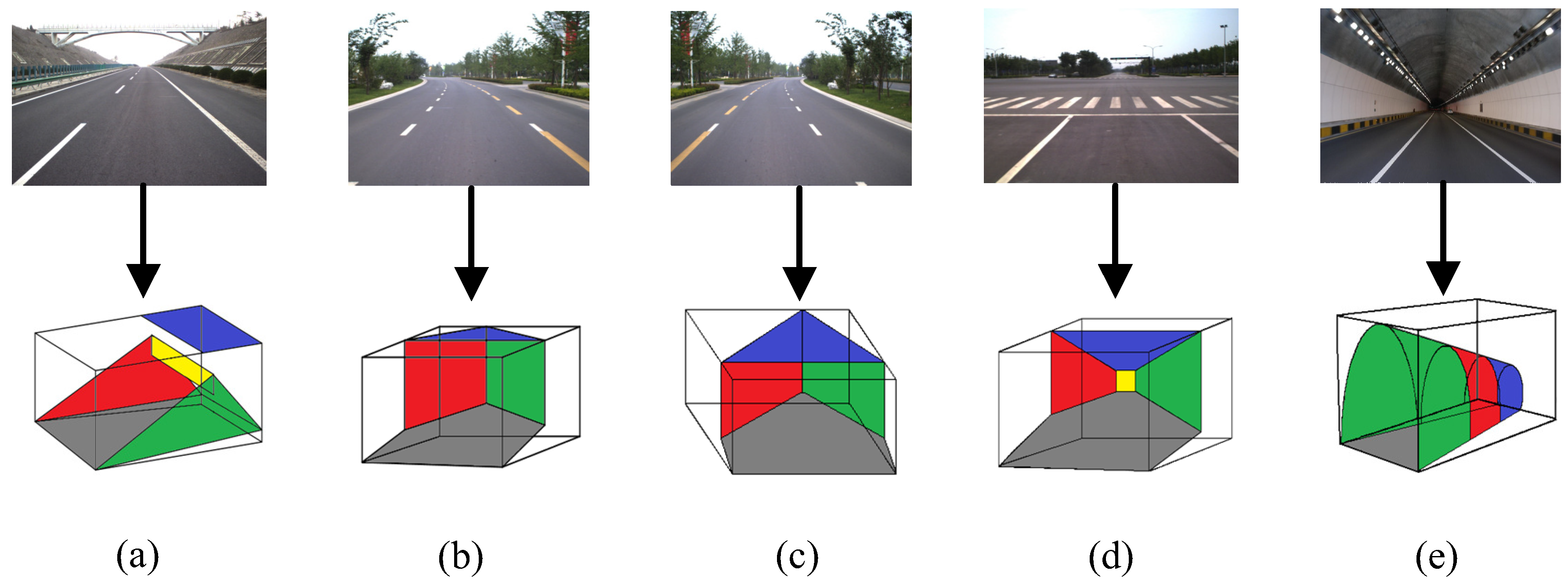
A set of scene stages
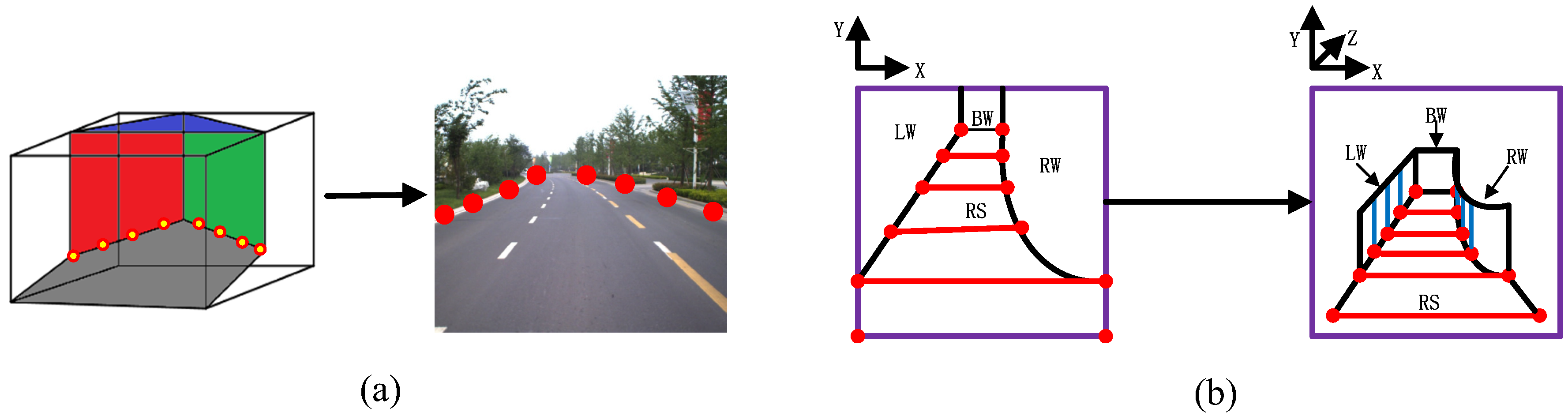
is defined in advance, which can represent the basic structures of typical road scenes. A related scene stage can be specified for each graph model to denote the scene’s geometric structure. The scene stage is a traffic scene wireframe model that represents the scene layout for 3D traffic scene modeling. Scene stages can be classified into simple and complex types, as shown in
Figure 5. A simple scene stage consists of just the background elements of a traffic scenes. A complex scene stage consists of both the background and foreground elements.
For the simple scene stages, the corresponding background models have a “floor-wall” structure, with the road region being located on the horizon plane. The rest of the background regions are assumed to be perpendicular to the road plane. For the complex scene stages, the foreground models are constructed from rectangular polygons, which are set vertically to the road plane. The foreground polygons have data structure, with A denoting the transparency ratio. The polygons in the region outside of the foreground are set to be transparent.
We determine the control points for the road boundaries according to the traffic scene wireframe model. The control points are distributed on both sides of the road. In each scene stage, the two farthest control points are taken from the far end of the road surface, while the two closest control points are specified by the near end of the road surface. The remaining control points are distributed between the farthest and the nearest control points, as shown in
Figure 6a. A 3D corridor road scene model can then be constructed according to the control points (this principle is shown in
Figure 6b). In addtion to traditional scene models, cartoon scene models can be constructed by applying non-photorealistic rendering to the input images [
28]. The road scene model construction process is summarized in Algorithm 2.
| Algorithm 2 Road scene model construction. |
Require: The region detection results for the image frames .
- 1:
for to M do - 2:
Specify the foreground regions and road region from ; - 3:
Construct the scene graph model ; - 4:
Specify the scene stage according to the scene graph model G; - 5:
Perform the scene construction based on the geometric structure of . - 6:
end for
Ensure: Road scene models with the “floor-wall” structure. |
4.2. Road Scene Simulation
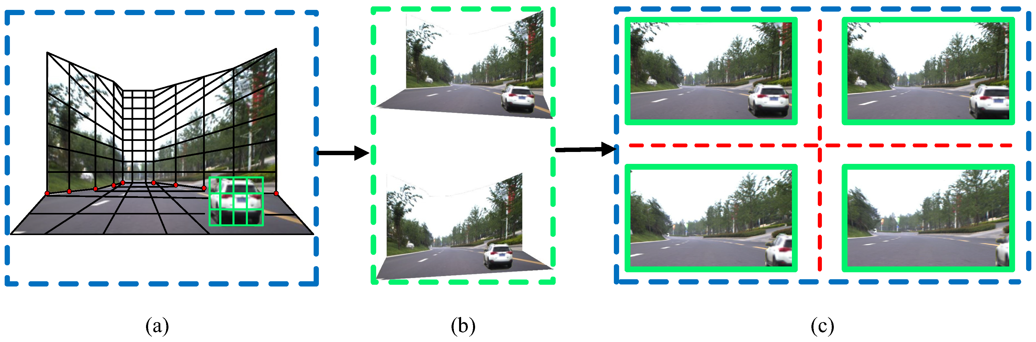
The 3D traffic scene simulation can be performed by assembling the “floor-wall”-structured scene model. The viewpoint can be freely changed during the simulation process by using the commands forward, back, up and down. With the assistance of GPS data, the trajectory of the viewpoint can be displayed on the map. Depending on how the viewpoint moves, the traffic scene simulation can be classified into two modes: (1) Roaming mode, where new viewpoint images are generated according to the movement of the viewpoint; (2) Bird’s-eye view mode, where the viewpoint is static and virtual vehicles and obstacles can be added into the scene. The generation of new viewpoint images is shown in
Figure 7a. The black grid represents the basic scene model. The green grid denotes the foreground vehicle model. Users can change the viewing angle through adjustments of the road scene model. The new viewpoint images are then generated, as shown in
Figure 7b.
We have designed five metrics for the offline testing of unmanned vehicles, namely: pedestrian recognition; collision avoidance; traffic signal recognition; pavement identification; and fog recognition. Four levels of performance for each metric were also defined to evaluate vehicle behavior, (L0, L1, L2, L3), as shown in
Table 3. The complexity of the road scene can generally be divided into three categories, (R1, R2, R3), according to: road conditions; special areas; and special kinds of weather. On the basis of these categories, various scenes can be constructed easily for the offline testing of unmanned vehicles. The three categories of road complexity are as follows:
R1: Different road conditions including rural roads, urban roads, highways and tunnels. The road parameters relate to the specific road width, the number of obstacles, traffic signs and traffic lights.
R2: Special areas including campuses, hospitals, crowded streets, etc. Vehicles in special areas need to react quickly and perform different operations.
R3: Special kinds of weather including rain, snow, fog, etc. The special kinds of weather may also be of varying degree. This needs to be accurately identified for the evaluations.
Finally, the performance of unmanned vehicles may be evaluated across a combination of different degrees of scene complexity and different evaluation metrics.
5. Experiments and Comparisons
Our experiments were undertaken on a computer with an Intel i5 processor @3.33 GHZ and with 16 GB Memory). The experimental data was mostly taken from the TSD-max dataset [
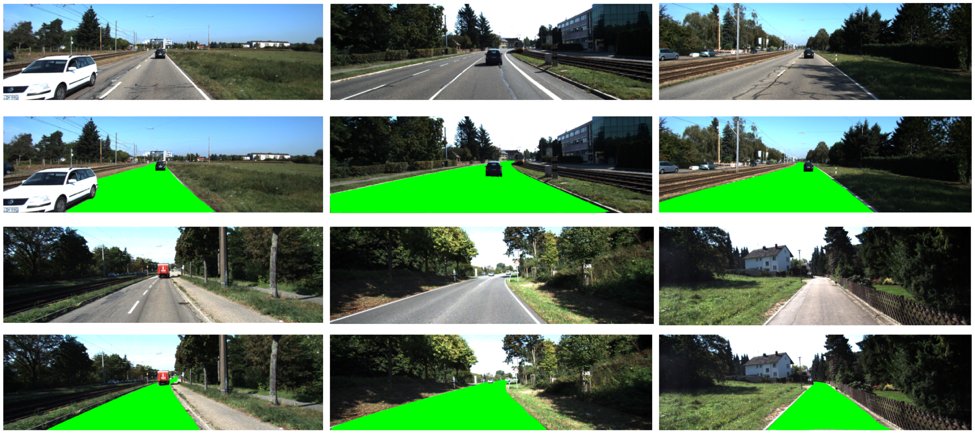
29], which was constructed by the Institute of Artificial Intelligence and Robotics at Xi’an Jiaotong University in China. The dataset is composed of road images captured from urban roads, rural roads, highways, etc. Specifically, the experiment of road region detection is also based on the KITTI dataset [
12].
5.1. Evaluation of the Region Detection
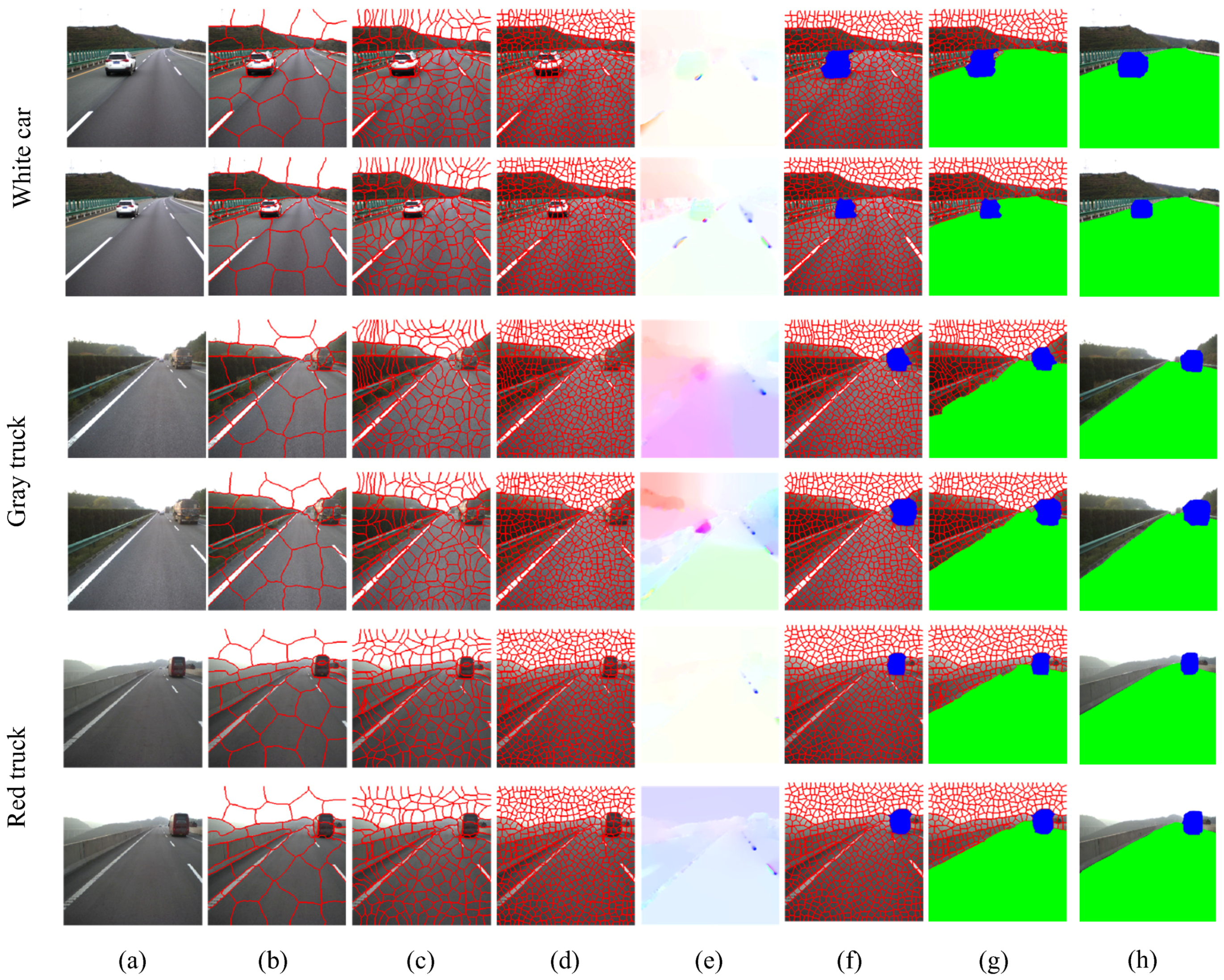
First of all, we perform the region detection experiments. Three image sequences are selected for the region detection experiments: White Car (512 × 512 pixel size, 200 frames), Gray Truck (512 × 512 pixel size, 300 frames), and Red Truck (512 × 512 pixel size, 250 frames). The KITTI dataset is utilized for the task of road region detection (1242 × 375 pixel size, 200 frames).
Figure 8 shows the superpixel segmentation at different scales, the optical flow map between adjacent frames, and the region detection results before and after refinement. The road detection results based on the superpixel-level RW method with refinement for the KITTI dataset is shown in
Figure 9. The algorithms mainly work on the basis of a superpixel segmentation size of
. For quantitative evaluation, we use three metrics: precision; recall; and F-measure to compare with the ground truth road and foreground regions. Precision denotes the ratio of correct pixels within the detected road region. Recall denotes the ratio of correct pixels in relation to the benchmark road region. In our experiments, precision and recall are defined as follows:
where
R and
denote the detected region and ground truth, respectively.
The
F-Measure can be computed by combining
Pre and
Rec:
We set
to give precision and recall equal weight.
We employ the superpixel SVM [
17], Markov random field (MRF) [
7], GrowCut [
8] and Siogkas’s RW [
9] as baseline methods for road region detection. Besides these methods, VGG16 [
15] and ResNet101 [
14] are implemented for the comparison of road detection results. The average values for all of the image sequences are shown in
Table 4 and
Table 5. With regard to the methods presented in this paper, the superpixel-level random walk (SRW) and the superpixel-level RW with level set refinement (SRW+Refine) are implemented. As the results of the comparisons show, the accuracy our proposed method is approximately similar to ResNet101, which is superior to the other baseline methods.
5.2. Evaluation of the Scene Construction
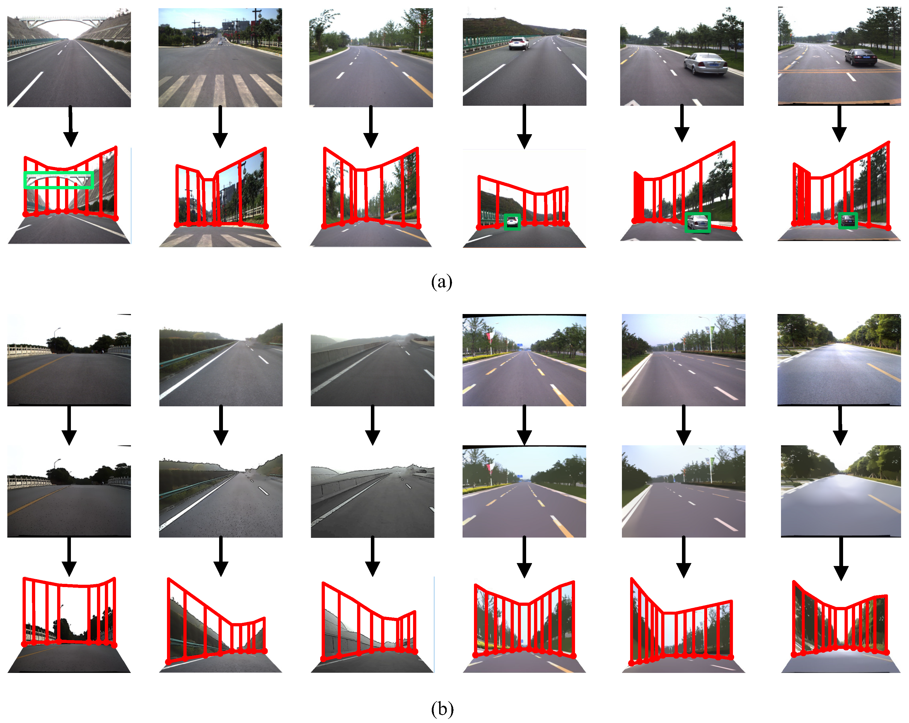
Next, we performed experiments relating to the scene construction and simulation. Input image sequences with a resolution of 1024 × 1024 pixels were once again selected from the TSD-max dataset, as shown in
Figure 10. There were three main types of scene models: (1) simple scene models based on pure background images; (2) complex scene models based on both foreground and background images; and (3) cartoon scene models based on non-photorealistic images [
28].
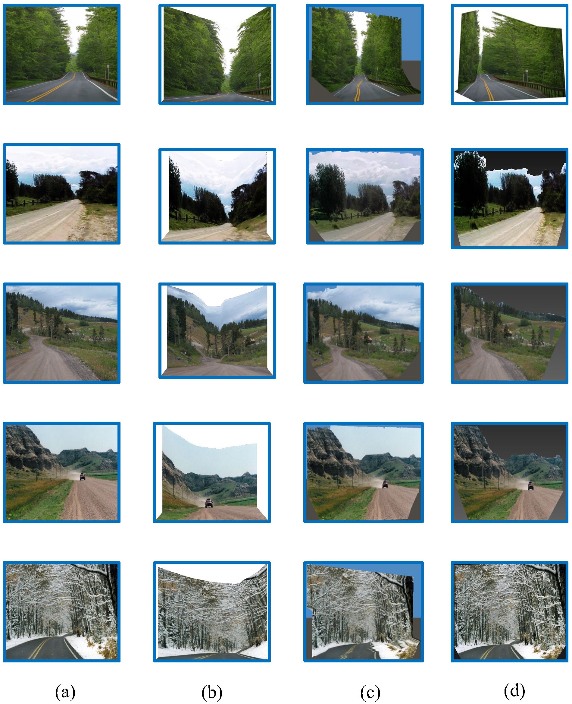
The scene models generated by our own approach were compared to those generated by Make3D [
16] and Photo Pop-up [
17], as shown in
Figure 11. The results demonstrate that distortions can occur in the Make3D and Photo Pop-up models. When compared to these baseline methods, our own approach produce the most realistic results. We also find that our proposed scene structure is more suitable for curved road conditions.
To qualitatively evaluate the scene models, we apply two metrics [
16]: (1) a plane correctness ratio, with a plane being defined as correct if more than 75% of the plane patches are correctly detected as semantic wall and road regions; (2) a model correctness ratio, with a model being defined as correct if more than 75% of the patches in the wall and the road planes had the correct relationship to their neighbors. The evaluation is performed by someone who is not associated with the project. One-thousand road images with a resolution of 1024 × 1024 are chosen overall. The comparative results according to these metrics are shown in
Table 6. As can be seen, the proposed scene models outperform the baseline methods in terms of both plane and model correctness.
6. Conclusions and Future Works
In this paper, we have proposed a framework for road scene model construction via superpixel-level RW region detection. The RW detection is able to locate road and foreground regions simultaneously. After segmentation of the superpixels, a region seed for the first frame is specified through user annotation. For each subsequent frame, the region seeds are located using trapezoids propagated from the previous frame. The RW algorithm is implemented through initialization of the region seeds, with the superpixels being utilized as graph nodes. In order to achieve more accurate region detection results, an FTC level set algorithm was also implemented for region refinement. After detection of the road and foreground regions, 3D corridor-style scene models can be constructed, depending on the type of scene stage. 3D traffic scene simulations can then be developed that are based on the scene models.
In the future research, we intend to use depth maps to construct more detailed scene models. A multi-view registration of point clouds can then be implemented to reconstruct 3D foreground structures. Cuboid models of the traffic elements can also be constructed on the basis of this for an even more sophisticated simulation of traffic scenes.


