Intention Estimation Using Set of Reference Trajectories as Behaviour Model

Abstract
1. Introduction
1.1. Contributions
1.2. Structure of the Paper
2. Method
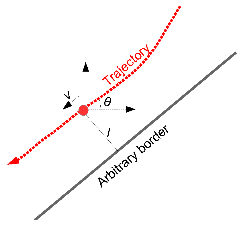
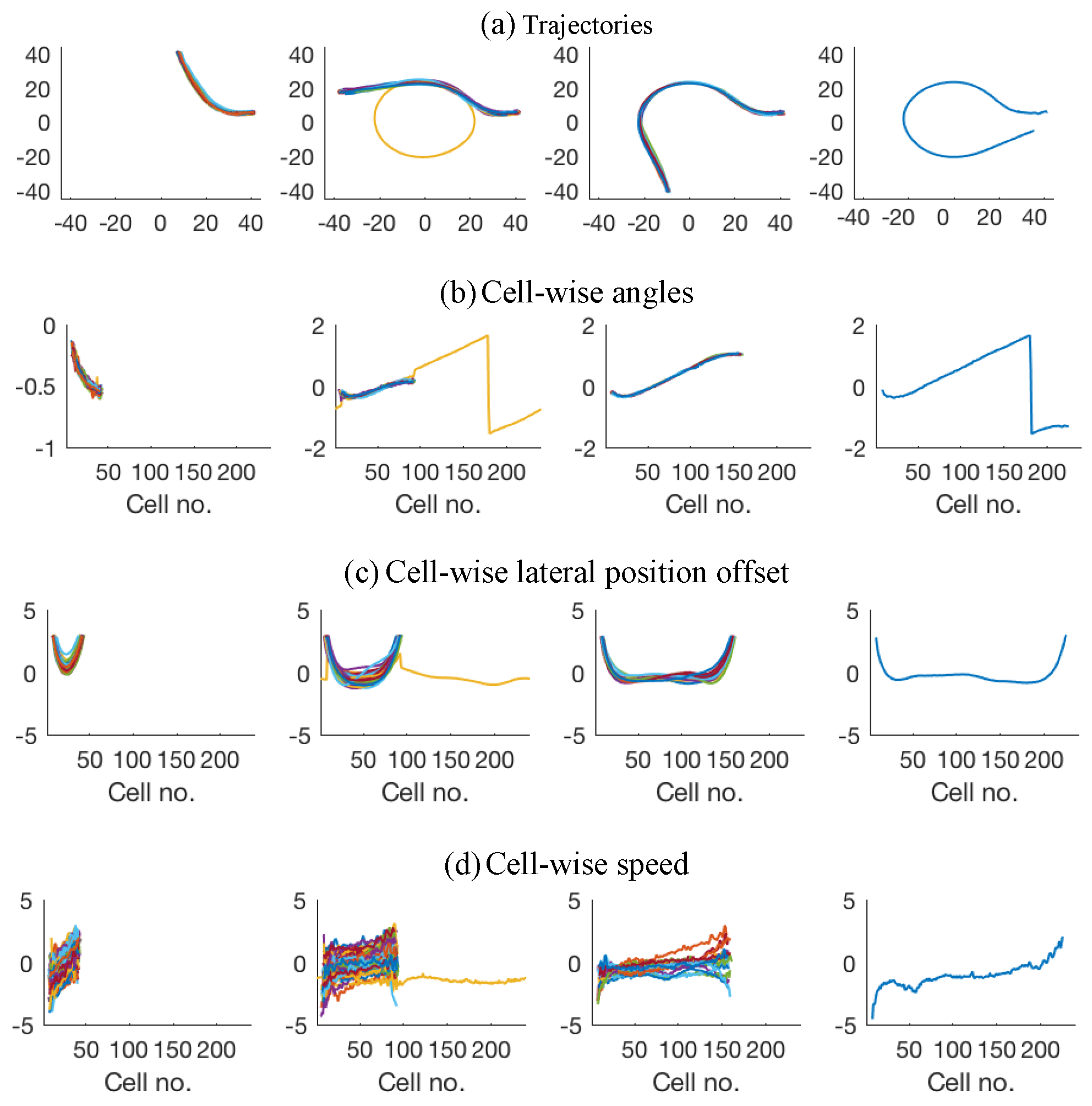
2.1. Behaviour Model
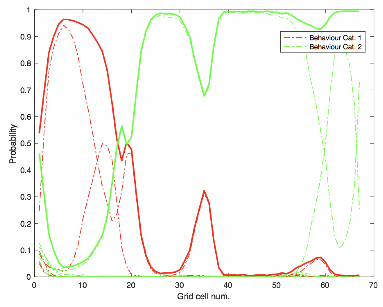
2.2. Using Particle Filtering
- Make the observation , i.e., measuring the feature value at current grid location of the query instance.
- Calculate the weight factor for each particle depending on how consistent the current measurement is with each of map trajectories.This is implemented by calculating the Euclidean distance between and the corresponding feature value in each of the map trajectories.
- Draw, with replacement, m particles from the updated particle set, with probability equal to particles’ associated importance weights to create updated particle set . Many alternative resampling methods also exist in the literature and an in-depth study on such methods is presented in [27].
2.3. Using Decision Trees
2.4. Validation Method
3. Results
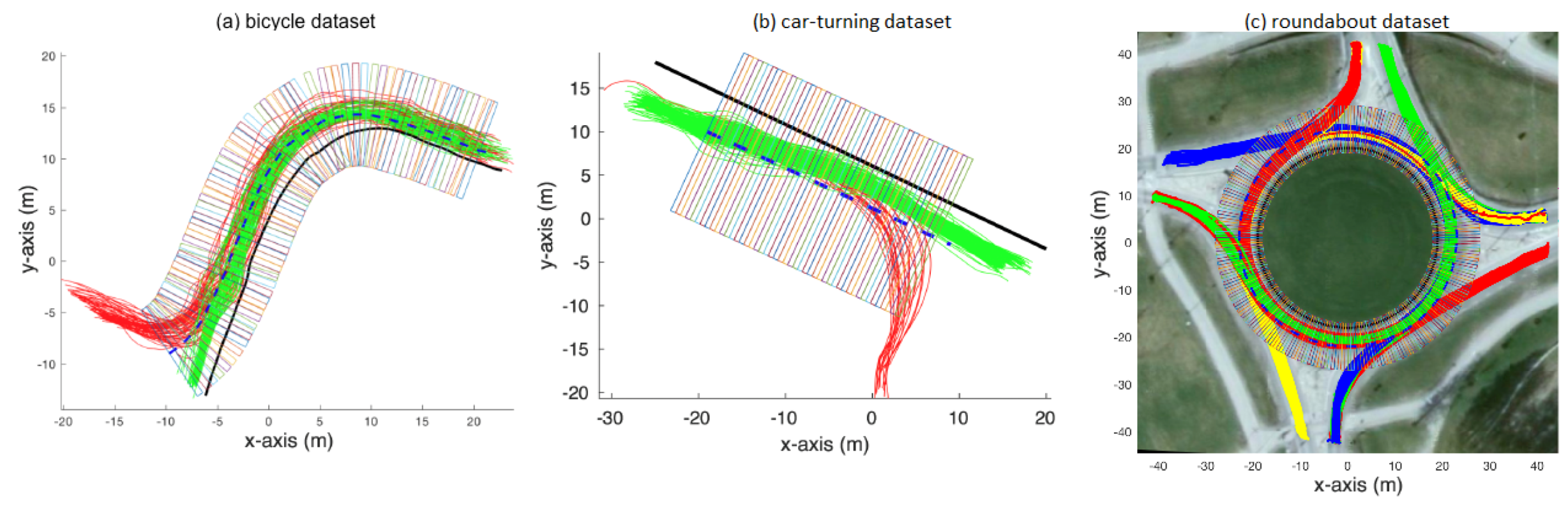
3.1. Data
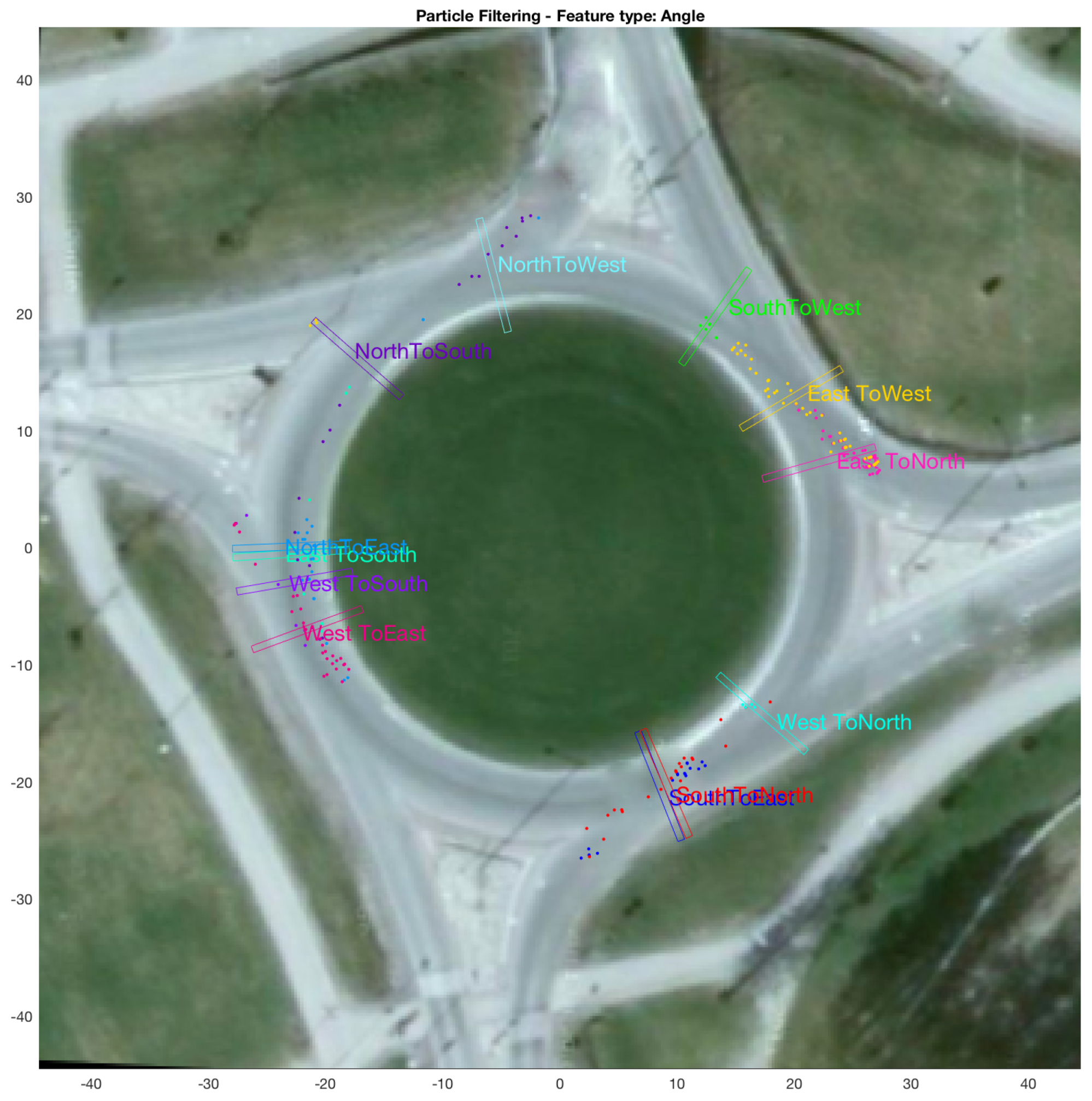
3.2. Basic Experiment Using Particle Filtering
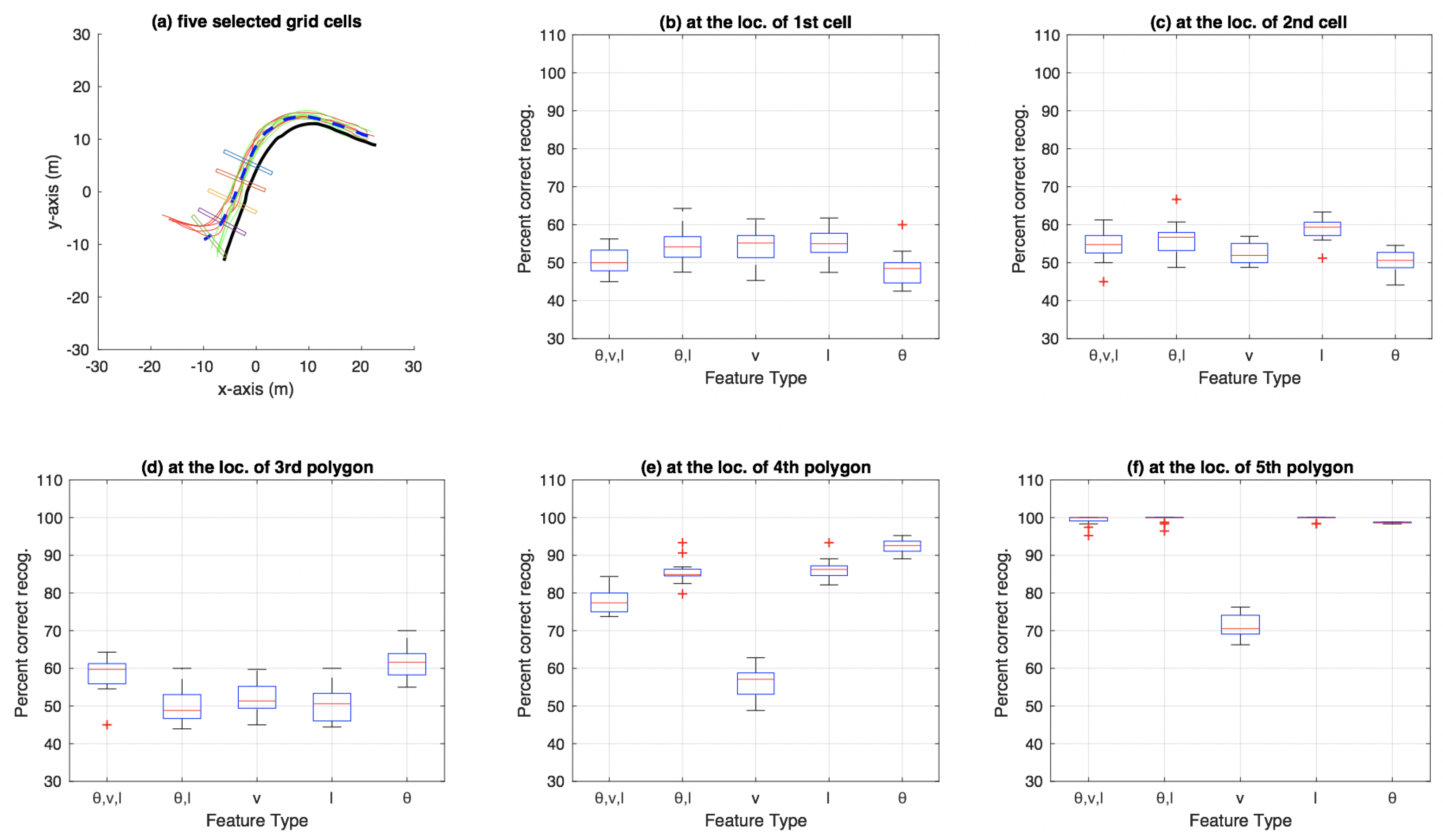
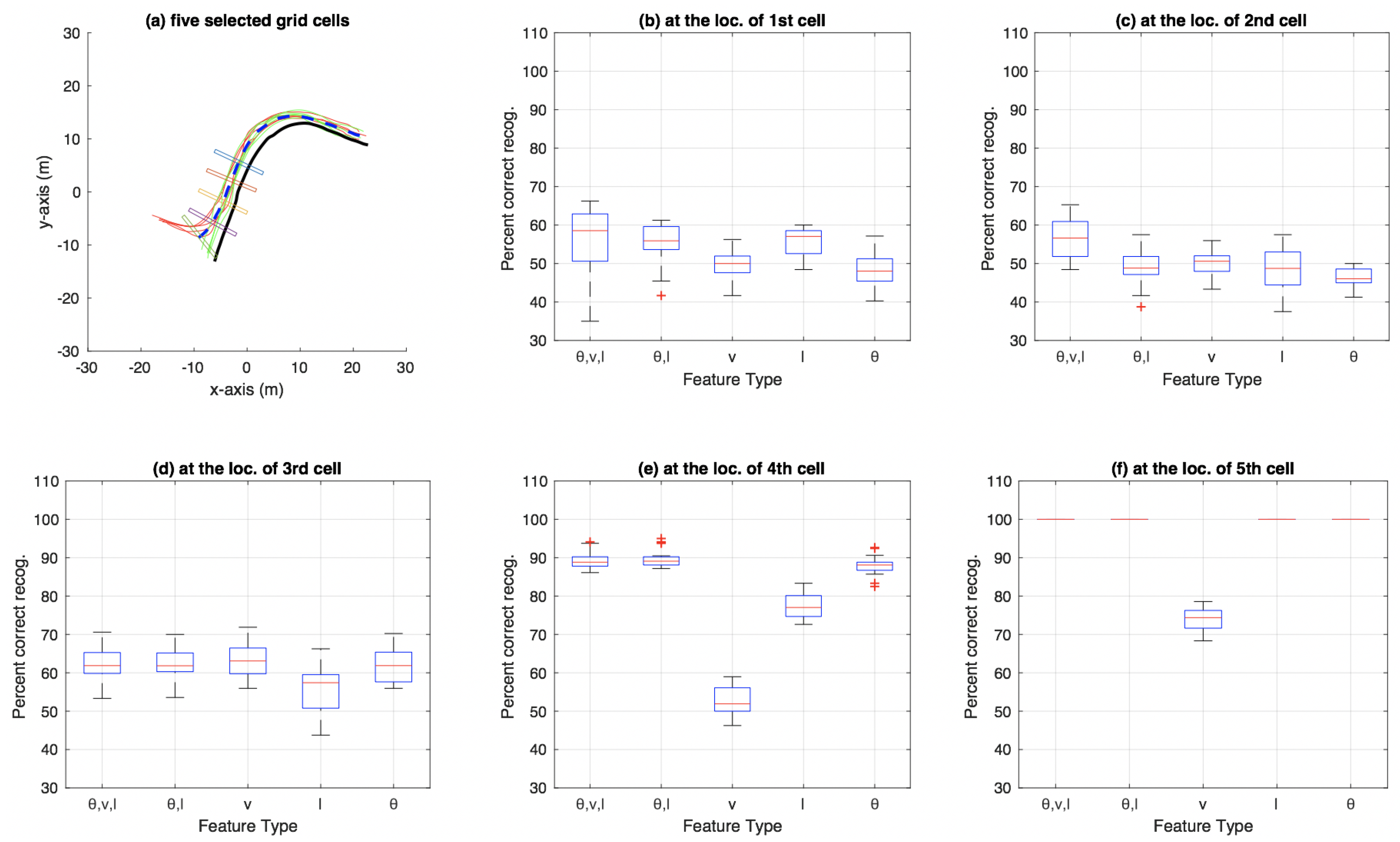
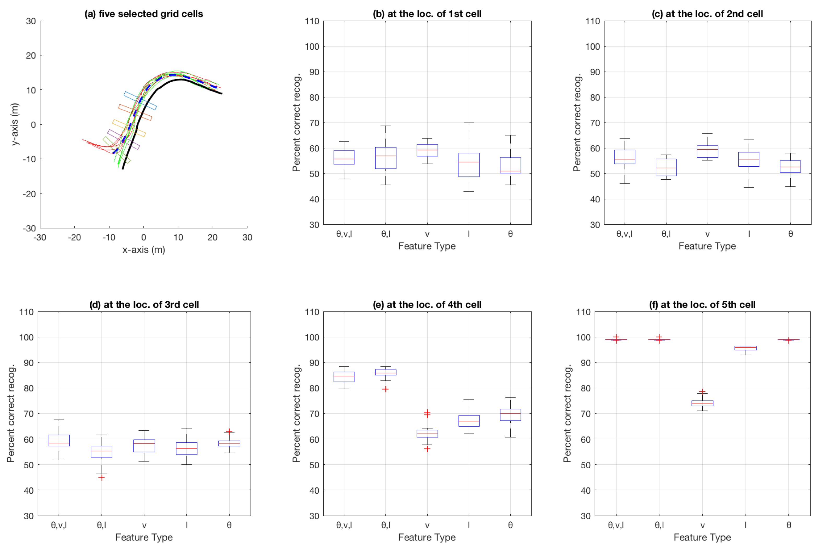
3.3. Aggregate Results Using Particle Filtering
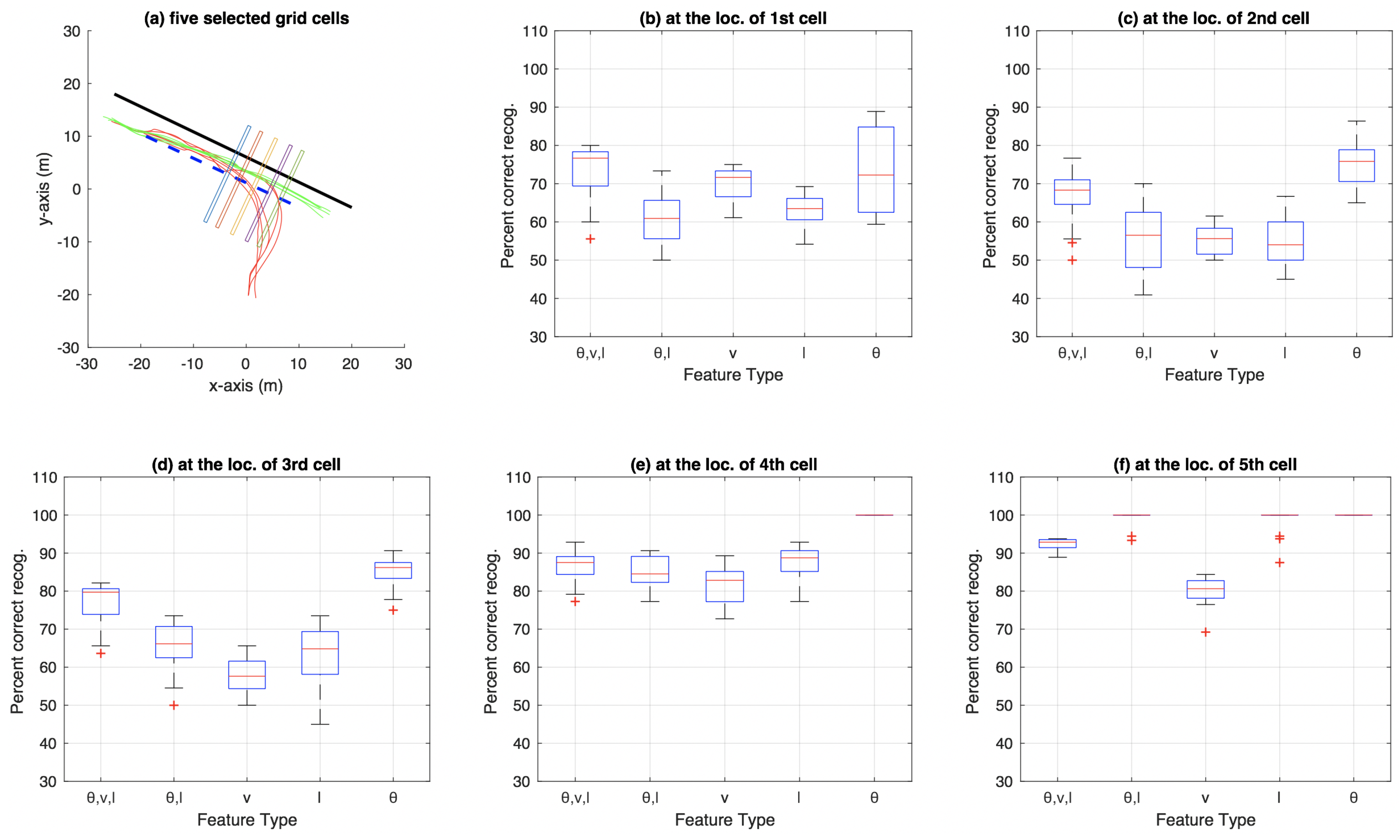
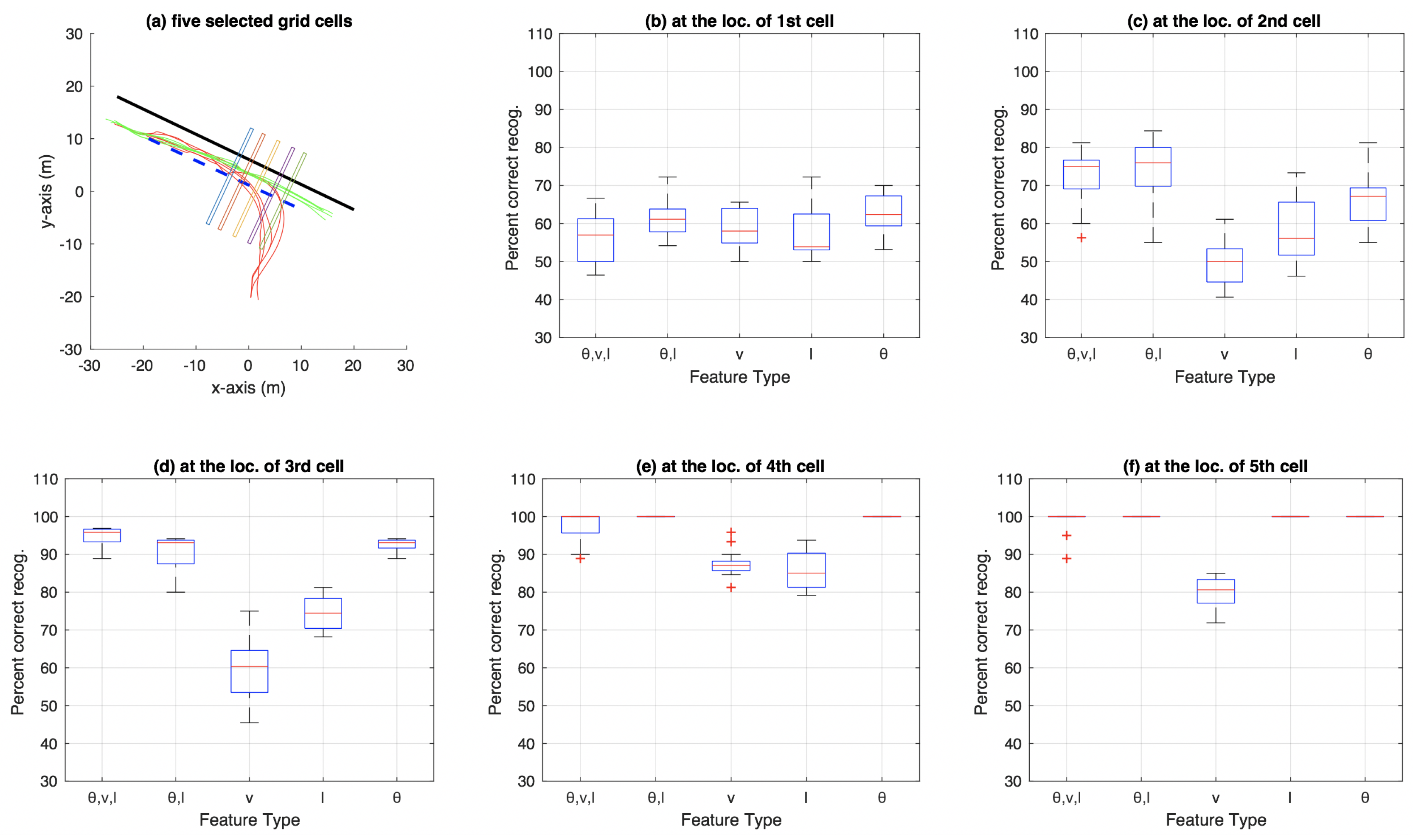
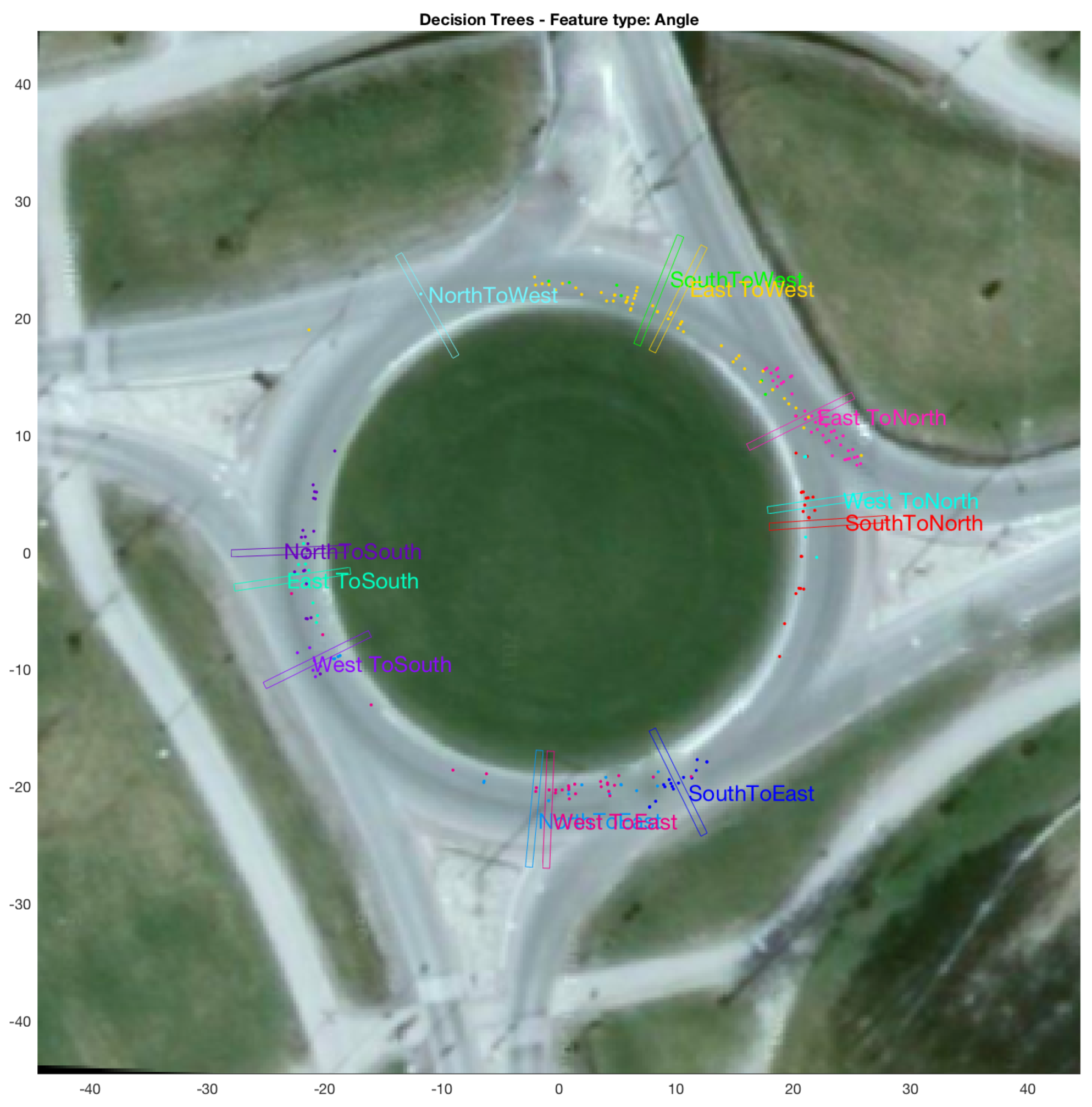
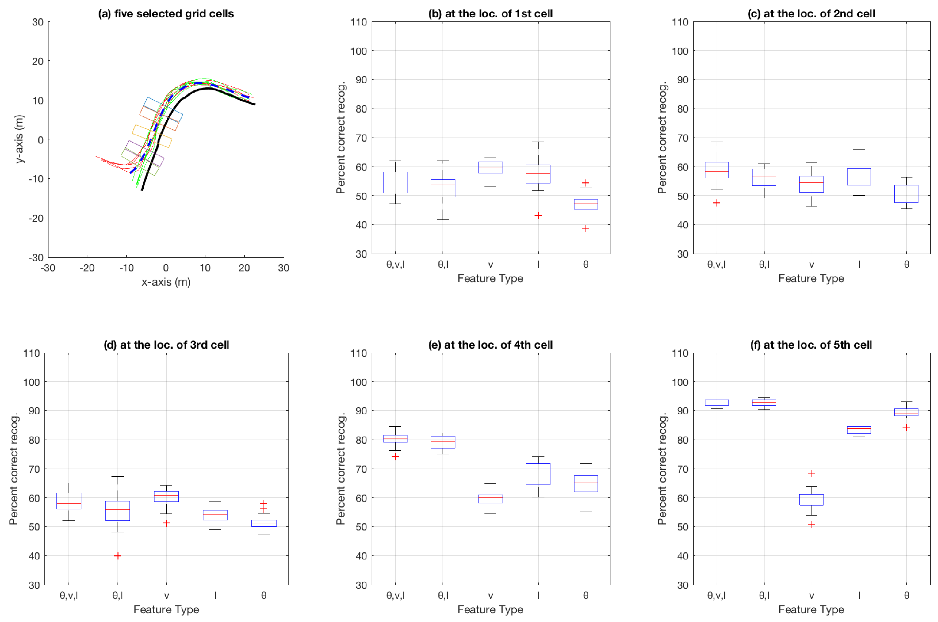
3.4. Aggregate Results Using Decision Trees
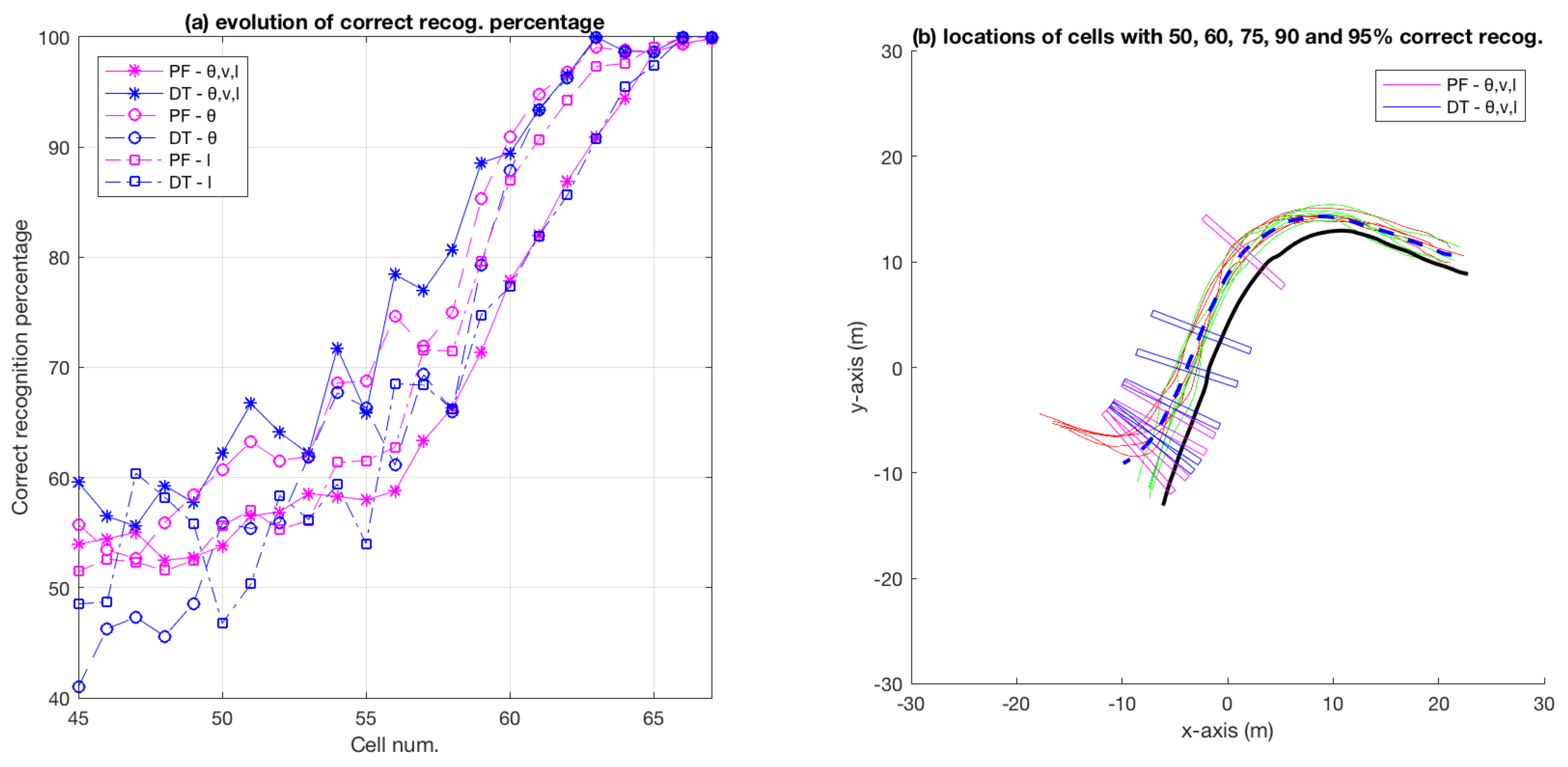
3.5. Results Comparing Particle-Filer and Decision-Tree Methods on Roundabout Dataset
4. Discussion
4.1. Speed as an Attribute
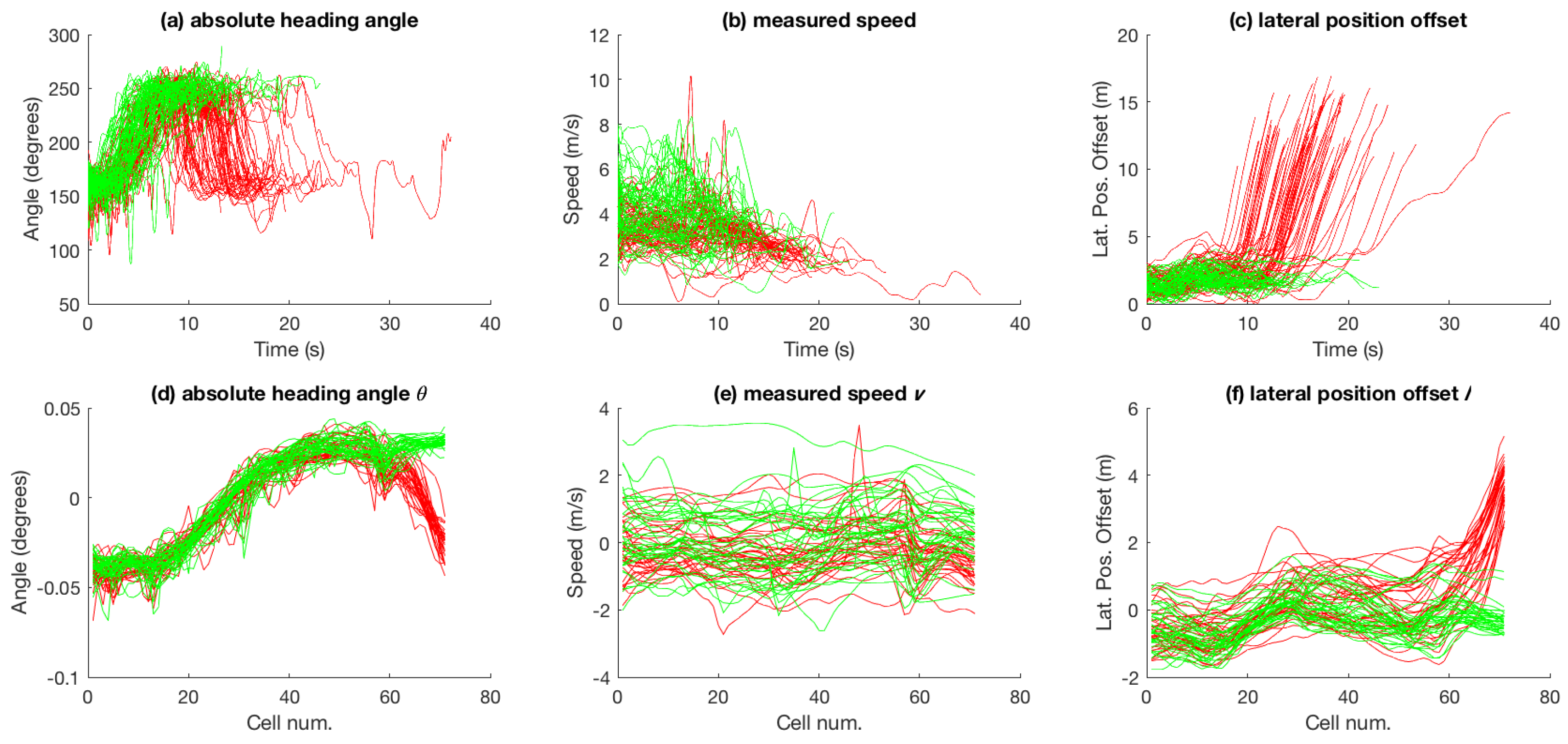
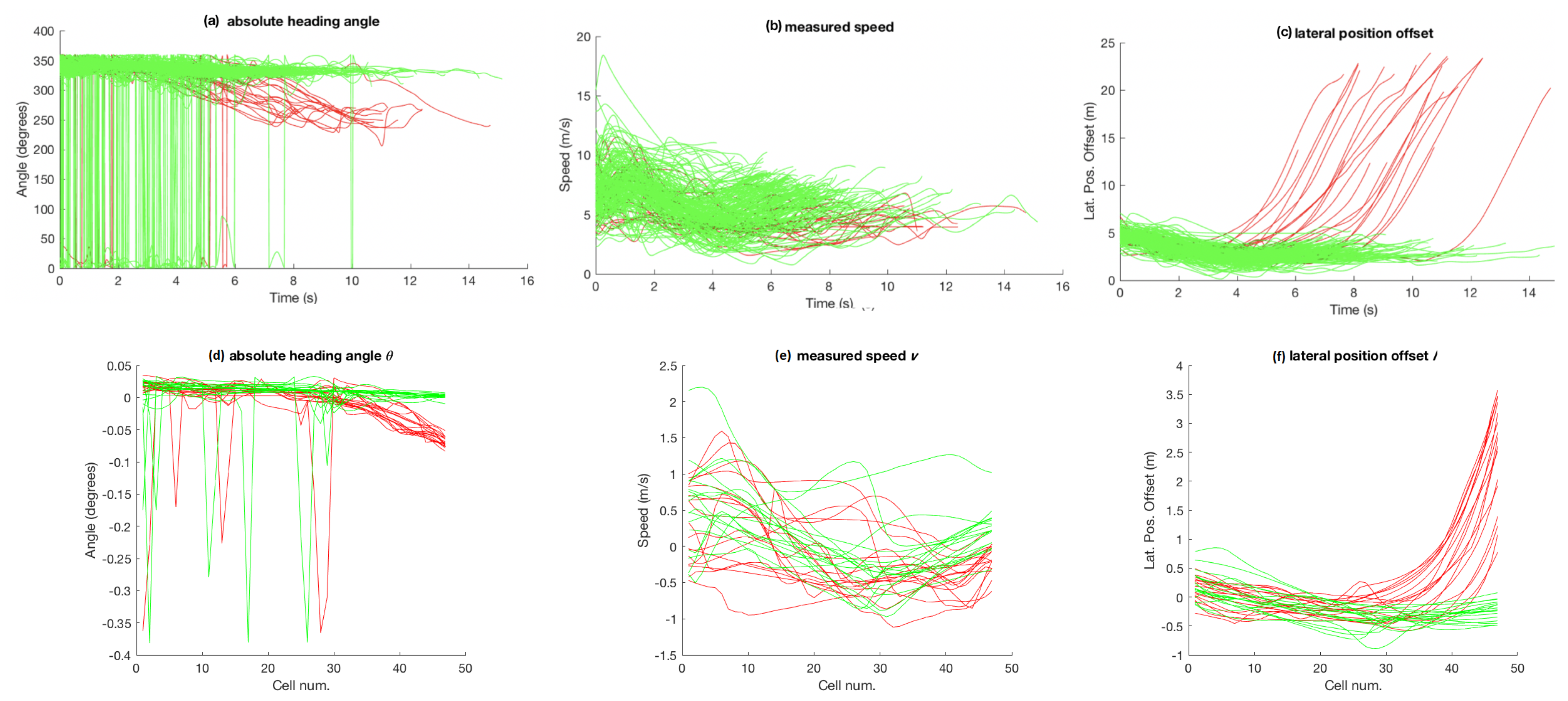
4.2. Performance of , l and (, v, l) as Feature
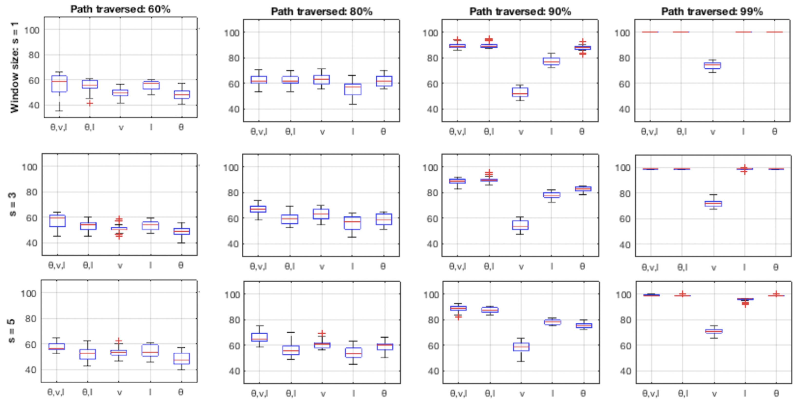
4.3. Cell Size
4.4. Incorporating History vs. Local Snapshots
4.5. Overall Performance of Particle-Filter and Decision-Tree Based Methods
4.6. Utility and Applications of Intention Estimation
5. Conclusions
Author Contributions
Funding
Acknowledgments
Conflicts of Interest
References
- Brooks, R. The Big Problem with Self-Driving Cars Is People. IEEE Spectr. Available online: https://spectrum.ieee.org/transportation/self-driving/the-big-problem-with-selfdriving-cars-is-people (accessed on 14 December 2018).
- Kwak, J.Y.; Ko, B.C.; Nam, J.Y. Pedestrian intention prediction based on dynamic fuzzy automata for vehicle driving at nighttime. Infrared Phys. Technol. 2017, 81, 41–51. [Google Scholar] [CrossRef]
- Lidström, K.; Larsson, T. Model-based Estimation of Driver Intentions Using Particle Filtering. In Proceedings of the 11th International IEEE Conference on Intelligent Transportation Systems, Beijing, China, 12–15 October 2008. [Google Scholar]
- Lidström, K.; Larsson, T. Act normal: Using uncertainty about driver intentions as a warning criterion. In Proceedings of the 16th World Congress on Intelligent Transportation Systems, Stockholm, Sweden, 21–25 September 2009. [Google Scholar]
- Li, S.; Wang, W.; Mo, Z.; Zhao, D. Cluster Naturalistic Driving Encounters Using Deep Unsupervised Learning. arXiv, 2018; arXiv:1802.10214. [Google Scholar]
- Liebner, M.; Baumann, M.; Klanner, F.; Stiller, C. Driver intent inference at urban intersections using the intelligent driver model. In Proceedings of the IEEE Intelligent Vehicles Symposium, Madrid, Spain, 3–7 June 2012. [Google Scholar]
- Martinez, C.M.; Heucke, M.; Wang, F.Y.; Gao, B.; Cao, D. Driving Style Recognition for Intelligent Vehicle Control and Advanced Driver Assistance: A Survey. IEEE Trans. Intell. Transp. Syst. 2018, 19, 666–676. [Google Scholar] [CrossRef]
- Jain, A.; Koppula, H.S.; Raghavan, B.; Soh, S.; Saxena, A. Car that Knows Before You Do: Anticipating Maneuvers via Learning Temporal Driving Models. In Proceedings of the IEEE International Conference on Computer Vision, Santiago, Chile, 13–16 December 2015. [Google Scholar]
- Maghsood, R.; Johannesson, P. Detection of steering events based on vehicle logging data using hidden Markov models. Int. J. Veh. Des. 2016, 70, 278–295. [Google Scholar] [CrossRef]
- Okamoto, K.; Berntorp, K.; Cairano, S.D. Driver Intention-based Vehicle Threat Assessment using Random Forests and Particle Filtering. Int. Fed. Autom. Control 2017, 50, 13860–13865. [Google Scholar] [CrossRef]
- Bokare, P.S.; Maurya, A.K. Acceleration-Deceleration Behaviour of Various Vehicle Types. In Proceedings of the World Conference on Transport Research, Shanghai, China, 10–15 July 2016. [Google Scholar]
- Maurya, A.K.; Bokare, P.S. Study of deceleration behaviour of different vehicle types. Int. J. Traffic Transp. Eng. 2012, 2, 253–270. [Google Scholar] [CrossRef]
- Alonso, J.D.; Vidal, E.R.; Rotter, A.; Muhlenberg, M. Lane-Change Decision Aid System Based on Motion-Driven Vehicle Tracking. IEEE Trans. Veh. Technol. 2008, 57, 2736–2746. [Google Scholar] [CrossRef]
- Sivaraman, S.; Morris, B.; Trivedi, M. Learning multi-lane trajectories using vehicle-based vision. In Proceedings of the IEEE International Conference on Computer Vision Workshop, Barcelona, Spain, 6–13 November 2011. [Google Scholar]
- Dong, C.; Dolan, J.M.; Litkouhi, B. Intention estimation for ramp merging control in autonomous driving. In Proceedings of the IEEE Intelligent Vehicles Symposium, Los Angeles, CA, USA, 11–14 June 2017; pp. 1584–1589. [Google Scholar]
- Kucner, T.; Saarinen, J.; Magnusson, M.; Lilienthal, A.J. Conditional transition maps: Learning motion patterns in dynamic environments. In Proceedings of the IEEE International Conference on Intelligent Robots and Systems, Tokyo, Japan, 3–7 November 2013. [Google Scholar]
- Tango, F.; Botta, M. ML Techniques for the Classification of Car-Following Maneuver. In AI*IA 2009: Emergent Perspectives in Artificial Intelligence; Serra, R., Cucchiara, R., Eds.; Springer: Berlin/Heidelberg, Germany, 2009; pp. 395–404. [Google Scholar]
- Salomonson, I.; Rathai, K.M.M. Mixed Driver Intention Estimation and Path Prediction Using Vehicle Motion and Road Structure Information. Master’s Thesis, Chalmers University of Technology, Gothenburg, Sweden, 2015. [Google Scholar]
- Zhao, M.; Kathner, D.; Jipp, M.; Soffker, D.; Lemmer, K. Modeling Driver Behavior at Roundabouts: Results from a Field Study. In Proceedings of the IEEE Intelligent Vehicles Symposium, Los Angeles, CA, USA, 11–14 June 2017. [Google Scholar]
- Zhao, M.; Kathner, D.; Soffker, D.; Jipp, M.; Lemmer, K. Modeling Driving Behavior at Roundabouts: Impact of Roundabout Layout and Surrounding Traffic on Driving Behavior. Workshop Paper. Available online: https://core.ac.uk/download/pdf/84275712.pdf (accessed on 8 December 2018).
- Sivaraman, S.; Trivedi, M.M. Looking at Vehicles on the Road: A Survey of Vision-Based Vehicle Detection, Tracking, and Behavior Analysis. IEEE Trans. Intell. Transp. Syst. 2013, 14, 1773–1795. [Google Scholar] [CrossRef]
- Cappé, O.; Godsill, S.J.; Moulines, E. An overview of existing methods and recent advances in sequential Monte Carlo. Proc. IEEE 2007, 95, 899–924. [Google Scholar] [CrossRef]
- Thrun, S.; Fox, D.; Burgard, W.; Dellaert, F. Robust Monte Carlo lozalization for mobile robots. Artif. Intell. 2001, 128, 99–141. [Google Scholar] [CrossRef]
- Wolf, J.; Burgard, W.; Burkhardt, H. Robust Vision-Based Localization by Combining an Image Retreival System with Monte Carlo Localization. IEEE Trans. Robot. 2005, 21, 208–216. [Google Scholar] [CrossRef]
- Arulampalam, M.S.; Maskell, S.; Gordon, N.; Clapp, T. A tutorial on particle filters for online nonlinear/non-Gaussian Bayesian tracking. IEEE Trans. Signal Process. 2002, 50, 174–188. [Google Scholar] [CrossRef]
- Doucet, A.; Johansen, A.M. A Tutorial on Particle Filtering and sMoothing: Fifteen Years Later; Oxford University Press: Oxford, UK, 2011. [Google Scholar]
- Li, T.; Bolic, M.; Djuric, P.M. Resampling Methods for Particle Filtering: Classification, implementation, and strategies. IEEE Signal Process. Mag. 2015, 32, 70–86. [Google Scholar] [CrossRef]
- Mitchell, T. Machine Learning; McGraw Hill: New York, NY, USA, 1997. [Google Scholar]
- Ho, T.K. Random Decision Forests. In Proceedings of the International Conference on Document Analysis and Recognition, Montreal, QC, Canada, 14–16 August 1995; pp. 278–282. [Google Scholar]
- Wang, Y.; Xiu, C.; Zhang, X.; Yang, D. WiFi Indoor Localization with CSI Fingerprinting-Based Random Forest. Sensors 2018, 18, 2869. [Google Scholar] [CrossRef] [PubMed]
- Verikas, A.; Gelzinis, A.; Bacauskiene, M. Mining data with random forests: A survey and results of new tests. Pattern Recognit. 2011, 44, 330–349. [Google Scholar] [CrossRef]
- Viscando Traffic Systems AB, Sweden. Available online: https://viscando.com/ (accessed on 14 December 2018).
- Fan, H.; Kucner, T.P.; Magnusson, M.; Li, T.; Lilienthal, A.J. A Dual PHD Filter for Effective Occupancy Filtering in a Highly Dynamic Environment. IEEE Trans. Intell. Transp. Syst. 2018, 19, 2977–2993. [Google Scholar] [CrossRef]


| Ground-Truth Exit | East | North | West | South | |
|---|---|---|---|---|---|
| Predicted Exit | |||||
| East (entering from N, W, S) | 76.25 | 5.76 | 1.78 | 26.94 | |
| North (entering from E, W, S) | 9.59 | 80.30 | 15.05 | 3.81 | |
| West (entering from E, N, S) | 4.52 | 13.71 | 82.80 | 4.81 | |
| South (entering from E, N, W) | 9.64 | 0.23 | 0.35 | 64.42 | |
| Ground-Truth Exit | East | North | West | South | |
|---|---|---|---|---|---|
| Predicted Exit | |||||
| East (entering from N, W, S) | 78.34 | 4.23 | 1.88 | 21.46 | |
| North (entering from E, W, S) | 10.99 | 88.53 | 12.42 | 1.01 | |
| West (entering from E, N, S) | 0.79 | 6.71 | 77.78 | 3.24 | |
| South (entering from E, N, W) | 9.87 | 0.53 | 7.92 | 74.29 | |
| Category | S-E | S-N | S-W | E-N | E-W | E-S | N-W | N-S | N-E | W-S | W-E | W-N |
|---|---|---|---|---|---|---|---|---|---|---|---|---|
| Leading method | PF | PF | PF | PF | PF | PF | PF | PF | PF | PF | PF | PF |
| Leading by (m) | 1.8 | 28.2 | 5.4 | 4.2 | 13.2 | 1.8 | 6 | 17.4 | 33 | 6.6 | 27 | 19.8 |
| Entry Direction (for an Eventual Exit at South) | East | North | West | |
|---|---|---|---|---|
| Predicted Exit | ||||
| (Number of test trajectories) | (5) | (30) | (5) | |
| East | 10.94 | 23.33 | 20.74 | |
| North | 5.26 | 0 | 2.86 | |
| West | 25.95 | 0 | 0 | |
| South | 57.84 | 76.67 | 76.41 | |
© 2018 by the authors. Licensee MDPI, Basel, Switzerland. This article is an open access article distributed under the terms and conditions of the Creative Commons Attribution (CC BY) license (http://creativecommons.org/licenses/by/4.0/).
Share and Cite
Muhammad, N.; Åstrand, B. Intention Estimation Using Set of Reference Trajectories as Behaviour Model. Sensors 2018, 18, 4423. https://doi.org/10.3390/s18124423
Muhammad N, Åstrand B. Intention Estimation Using Set of Reference Trajectories as Behaviour Model. Sensors. 2018; 18(12):4423. https://doi.org/10.3390/s18124423
Chicago/Turabian StyleMuhammad, Naveed, and Björn Åstrand. 2018. "Intention Estimation Using Set of Reference Trajectories as Behaviour Model" Sensors 18, no. 12: 4423. https://doi.org/10.3390/s18124423
APA StyleMuhammad, N., & Åstrand, B. (2018). Intention Estimation Using Set of Reference Trajectories as Behaviour Model. Sensors, 18(12), 4423. https://doi.org/10.3390/s18124423