With the link evaluation results, the decision model is proposed to solve the following three problems, first is whether a node itself is healthy(SCP), second is whether a node is the leader who is responsible for removing faulty nodes(LUP), third is which nodes are faulty(FNDP).
We denote the cluster (nodes and its links) to be a simple undirected graph
, where
. As shown in
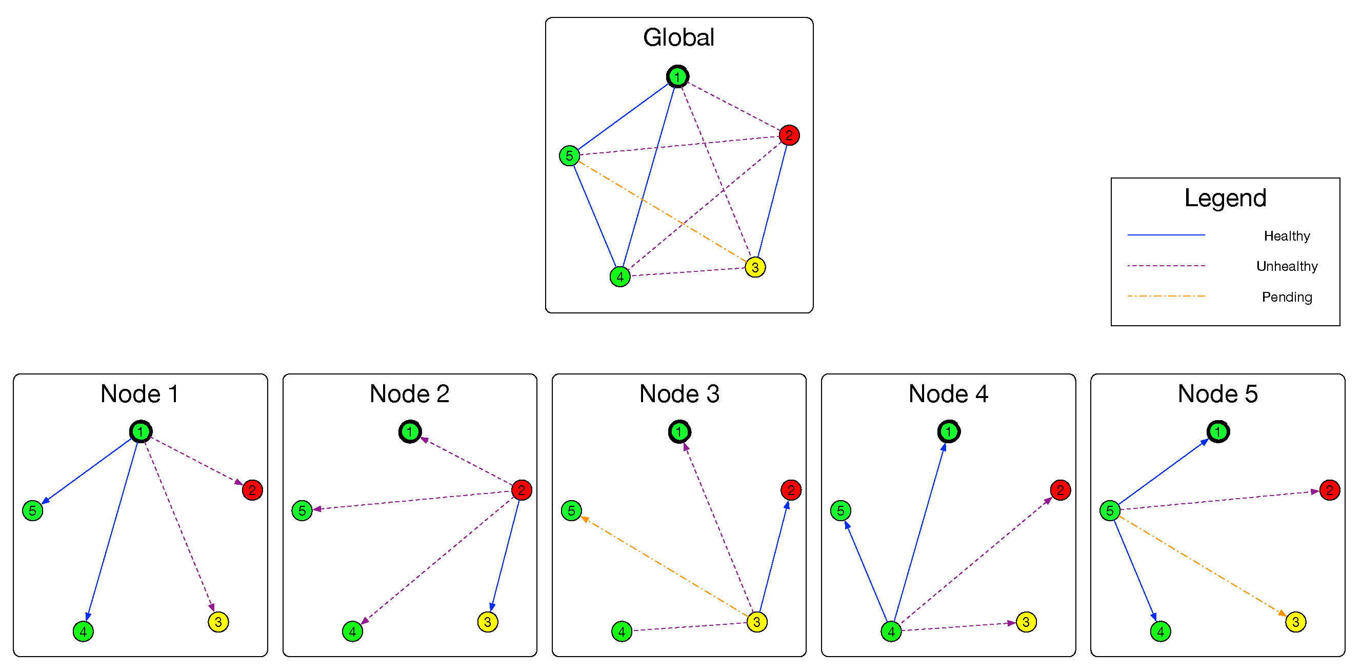
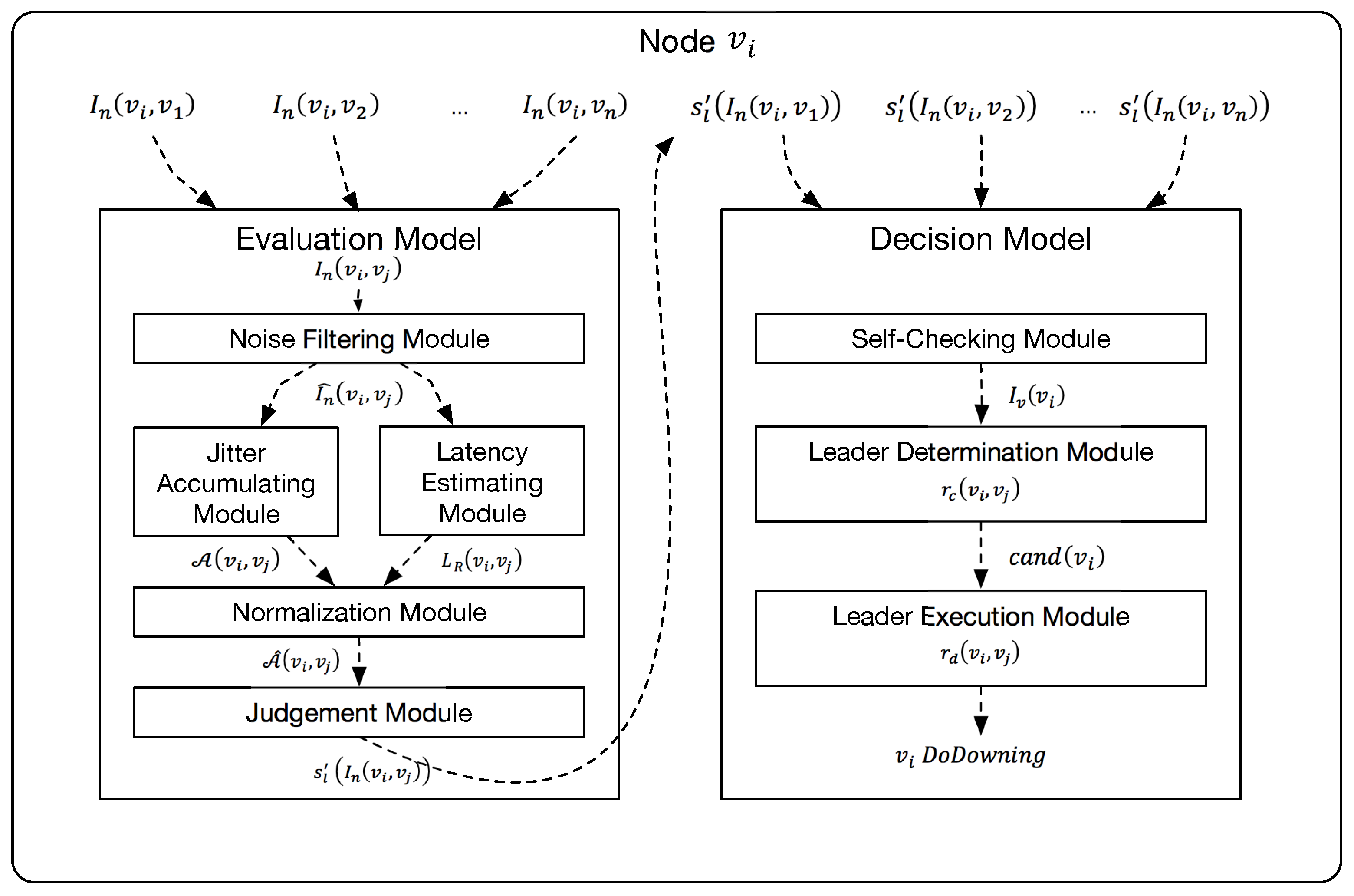
Figure 3, with the help of evaluation model, a node
can build a group of subgraphs
and
with the result of Evaluation model. Similar to the relationship between
and
,
(and also
) is the observation of
E. If an edge is in the set
, the evaluation result of this link is Healthy. As for edges existing in
, their evaluation results are Unhealthy. If an edge
is neither in
nor in
, its evaluation result is Pending. Formally,
and
are defined as follows:
Next, we present some definitions about the node state.
Particularly, when the transitivity is applicable, if a node is PendingHealty, it must be Healthy.
We use the following 3 modules to solve the problem of SCP, LUP and FNDP. They are used to check the state of local node, ensure the uniqueness of leader, construct a global as an approximation of graph G and remove faulty nodes based on , respectively.
4.2.1. Self-Checking Module
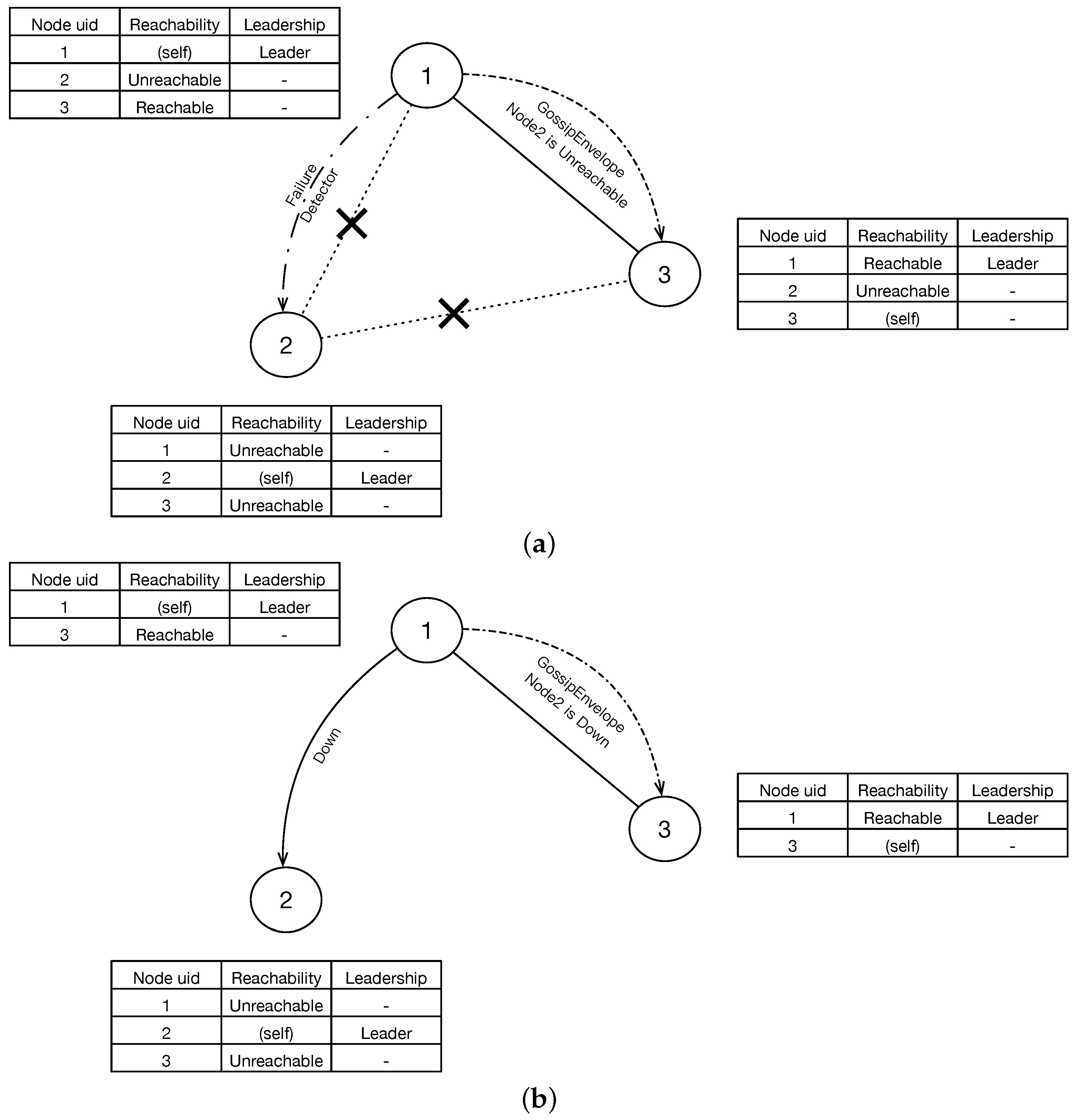
At any time, a faulty node should not be selected as the leader. However, the evaluation model or other failure detection mechanisms cannot sense which side, i.e., whether themselves or their peers, is faulty. We thereby design this module to do self-checking and if one’s self-checking procedure indicates that itself is faulty, it will abandon all the next steps and report this issue to the upper applications. More specifically, this module proposes the indicator and the function of .
With the basis of Lemma 1, Lemma 2 and Definition 5, we come up with the idea of this module that, if the majority of the nodes in the cluster announce that is the faulty one using the evaluation module, should be unhealthy. Although it is possible that all the announcers are unhealthy, however, in that case we can say that most of the nodes in the cluster have failed so that the cluster is totally out of function and it would be meaningless to discuss the reliability and availability. On the contrary of the condition of unhealthy, if the majority ones believe that is healthy, should be healthy although it is actually PendingHealthy which we have already discussed about.
This idea can then be described as:
Unfortunately, the self-checking process is performed in
, who has no knowledge about
and
,
. We thereby consider that
. Because
is expected,
is also expected due to transitivity. Combine with (
8) and (
9), we have the following theorem:
Theorem 2. If then and if then .
With Theorem 2, the function of
can be easily calculated locally because (
16) can be converted to:
If the self-checking result is healthy, this node should go forward to leader determination module. Otherwise, the node may suffer from network failure and it should handle this issue. If the result is pending, the node may do nothing but wait for more reliable link evaluation results.
4.2.2. Leader Determination Module
This module is to make healthy nodes find the cluster leader without election, i.e., find the function
. Recall
Table 1 (f), each node is given a unique id by function
. With the help of this function, the main idea of this module can be described as choosing the node from the healthy set with the minimal unique id to be the leader. Therefore, we define the basic candidate rule
to be:
However, in this case of the basic candidate rule, we can find that one
must obtain all remote nodes’ healthy states, i.e.,
for all
, which cannot be directly acquired locally. For this reason, an approach is needed to get or infer the status of remote nodes. Here we need to consider about the transitivity. Recall
Section 3.2, this property is applicable in most cases but do have exceptions. Hence, we propose two different approaches classified by the applicability of this property.
The first approach is to infer healthy states of remote nodes. In the most common conditions that transitivity is applicable, the two following theorems that can be proved:
Theorem 3. When transitivity is applicable, for an arbitrary node , if it has a healthy link that connected to a healthy node , must be healthy. This can be formulated as: Proof. Because
, according to Definition 4, we have:
Combine with (
19), transitivity (
2), and the fact that
, it can be inferred that
. Thus, we have:
According to Theorem 1 and (
20), the state of
can be demonstrated:
. ☐
Lemma 3. (With transitivity) For three nodes , and , if the link state from to is Healthy and that from to is Unhealthy, it can be inferred that the link state from to is Unhealthy. This lemma can be formulated to: Theorem 4. (With transitivity) For two nodes and , if the state of is Healthy, and the link between and is Unhealthy, it can be inferred that the state of is Unhealthy. Theorem 4 can be proved similar to the proof of Theorem 3.
Proof. According to Lemma 3 and (
19), because the link status
, we have inferred that
, which also can be expressed as
. Combine with Lemma 2, we can conclude that
. ☐
With Theorems 3 and 4, the state of a remote node can be easily inferred from the link evaluation results. In short, when the transitivity is applicable, if the state of a link starts with a healthy node is healthy, the destination remote node is in state of healthy. Hence the candidate rule
can be redefined to:
The second approach is fetching healthy states from remote nodes. In the condition that the transitivity is not applicable, we have to fetch all the partial topologies from remote nodes and combine them to a global topology. This helps us to choose a unique leader in this module and further help to do execution in the next module.
Recall the very first of this section, partial topology in node
are denoted by a group of directed graphs
and
and the global topology is denoted by an undirected graph
. For an arbitrary healthy node
, the target of this module is to fetch the remote partial
for
, and combine these
to an undirected graph
which is expected to be equal to
G. When a node successfully constructs
, it will be able to calculate the states of nodes using the approach provided in Self-Checking module. The candidate rule can then be defined as:
To introduce our approach in detail, we here make definitions on Healthy observation set and Unhealthy observation set of nodes.
Definition 6. Healthy observation set of an arbitrary node is the set of nodes that the link between them and is healthy, which can be expressed as .
Definition 7. Unhealthy observation set is defined as : .
For implementation, we also use to approximate in order to obtain the observed and in each node.
To combine the partial topologies into a global topology, we have to deal with the following issues (suppose the local node is ). First, fetches partial topologies from the nodes in directly. Then, asks for partial topologies of unreachable nodes, i.e., nodes in , with the help of nodes in . While fetching partial topologies, handle the ask timeout. While combining the partial topologies, check for and resolve the conflict state of a certain edge from two sides of nodes. Finally, give the combination result.
Algorithms 2–4 shows the full workflow of this module.
Algorithm 2 shows the workflow of fetching and combining process. This process is started by the initiator who tries to acquire the global topology. It first initializes a pair of mutable graphs , which will eventually hold the combination result, i.e., global graph; a mutable set , which indicates whose sub connectivity graphs have been combined into the the intermediate and , an immutable Healthy observation set . For all nodes in , it sends a AskTopo RPC to these nodes. If a ReplyTopo is replied, try to merge the replied graph with . If merging process succeeded, combine the returned seen set with the local seen set . If merging process failed, stop the fetching and combining process immediately and report the conflict issue. If no ReplyTopo is replied, mark the edge from the local node to this remote node as Unhealthy and also add this remote node into seen set.
Algorithm 4 shows the workflow when a node receives a AskTopo RPC. If the sender of this RPC asks for aid to grab sub connectivity graphs from other nodes in (because the sender cannot connect to these nodes), the receiver will invoke FetchAndCombine and set the parameter to be . If , the FetchAndCombine will do nothing but return its own sub graph. After FetchAndCombine process is completed, the receiver will pack the combine result into ReplyTopo message and send back to the sender of AskTopo RPC.
| Algorithm 2: Fetching and combining algorithm. FetchAndCombine(). |
![Sensors 18 00320 i002]() |
| Algorithm 3: Merging algorithm. Merge(). |
![Sensors 18 00320 i003]() |
| Algorithm 4: Replying algorithm. |
![Sensors 18 00320 i004]() |
Generally speaking, the workflow is that, the initiator starts the fetching process by calling FetchAndCombine(), which will send AskTopo RPCs to all reachable remote nodes. This will trigger the process of Algorithm 4 in all these remote nodes. All the receivers then try to reply to ReplyTopo messages containing their sub connectivity graphs and possibility containing the sub connectivity graphs of nodes cannot be reached by the sender. The function of FetchAndCombine will call the function Merge, which is presented in Algorithm 3, to merge different sub graphs after checking and resolving the conflict. Our default conflict resolving policy is that: if two sides give the detection result of an edge as a Pending and a non-Pending, the resolving result will be the non-Pending result; if two sides give the detection result of an edge as two different non-Pending results, the merging process will stop and give out the result of “conflict”.
For example, if
and
detects the edge
to be
and
, respectively, after merging, the edge will be marked as
which is to say the edge will appeared in the Healthy edge set
; if
and
detects the edge
to be
and
, respectively, merging will be interrupted.
Table 4 shows the detail of this policy.
4.2.3. Leader Execution Module
Leader node chosen by the former module uses leader execution module to find the set of
and removes these nodes in
from the cluster. Then, for a leader node
and an arbitrary remote node
, the downing rule can be described as follows:
We construct based on the idea that after the execution, the rest of the nodes can normally transmit data with each other, which is to say they form a complete graph from the perspective of graph theory. So we abstract the objective of this module to be (1) find a maximal clique, with best effort, a maximum clique, of , which means finding a subgraph of with maximal or maximum nodes satisfying the condition that is a complete graph; (2) let .
The MCP (max clique problem) is a NP-Complete problem [
24]. Therefore, we need an algorithm to reduce the computing complexity to make our algorithm available in big clusters. In this section, according to the applicability of transitivity, we propose two algorithms for each case. In the first case with the property, our algorithm will always find a max clique with the computing complexity of
. While in the second case without the property, we propose simple heuristic algorithm that will find a maximal (maybe max) clique with the computing complexity of
.
The first scenario is that the transitivity is applicable. In this case, the leader
can find a max clique by a very simple policy of:
This is because the theorem below can be proved.
Theorem 5. With the transitivity, a healthy node and all its peers end with healthy links construct the unique max clique of the global graph G.
Proof. We let
,
. We also introduce the notations of
,
,
,
,
G,
V,
E in Theorem 5 (
25).
Maximal proof:
Because the definition of means a set of nodes with unhealthy link state with at least one node in set , which can be expressed as: . We can then conclude that , the graph is not a complete graph, which means the graph is a maximal clique of the graph G.
Maximum and unique proof:
We denote
,
. If (
26) is true, and because
, we can infer that
,
. Then
,
,
s.t.
,
. Thus we have,
On the other hand,
,
s.t.
. According to Lemma 3, we have the inference that,
(
27) conflicts with (
28), thereby the assumption (
26) is false. Thus,
s.t.
. ☐
Therefore, in this case, the leader node
can simply construct the global
from
and
to approximate
G. With a loose policy that a leader will not remove a node with the link state of Pending between them, the
can be built with:
Finally, with (
24) and (
29), we find the set
:
The second scenario is that the transitivity is not applicable. In this case, we propose an easy-understanding, easy-implementing algorithm that will always find a maximal clique of G. Our idea is that, from the Self-Checking module, we can see that the healthy state of a node has strong correlation with . We therefore iteratively remove the node with worst state, i.e., minimal until the rest of the nodes are fully connected. Algorithm 5 shows the process of this algorithm in details.
| Algorithm 5: Finding a maximal clique. |
![Sensors 18 00320 i005]() |
After the leader get the clique
, it will find the set
to be:


