4.2. Modified Diffusion Wavelets
Conventional CS-based data-gathering approaches generally assume that sensor node readings have perfect sparse features under FFT, DWT, DCT, etc. To make full use of the spatial correlation property, which is demonstrated by experiments in
Section 4.1, we take diffusion wavelets [
36] as the sparse basis considering the spatial correlation of sensor node readings in WSNs. One is the nodes degree, and the other is the distance between the different sensor nodes. In addition, an improved QR decomposition of Givens transform is introduced to set up the sparse basis. Then, we describe how to construct the modified diffusion wavelets in detail. However, diffusion wavelets are affected significantly by the diffusion operator, which is equivalent to the wavelet function of a discrete wavelet transform. Diffusion is utilized as a smoothing and scaling technique to enable multi-scale and coarse-grained application. The detailed steps are shown in Algorithm 1.
Step 1: Suppose that
denotes a graph with
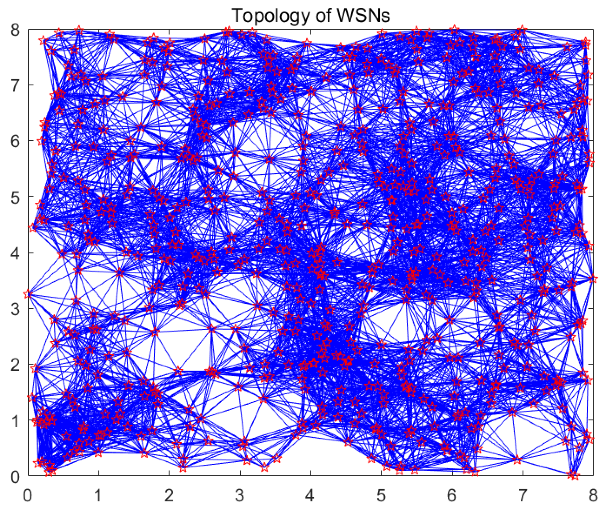
sensor nodes deployed in the monitoring environment, as indicated in
Section 3.2. Diffusion wavelets are introduced to set up an orthonormal basis for functions supported by the topology graph of WSNs. In this section, we take a random deployment of WSNs to explain this process. WSNs’ topology of 640 sensor nodes is shown in
Figure 3. In
Figure 3, the hexagram vertex represents the sensor node, while the blue edge denotes the wireless link.
Step 2: Calculate the weight adjacency matrix of
, which is denoted as
.
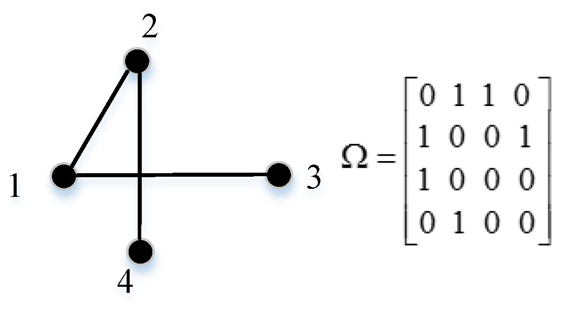
is the weight of the edge in the graph. In this section, we consider two different cases of weight. The sensor node degree is chosen as the weight in the first scheme, while the distance between sensor nodes is taken into consideration to exploit the spatial correlation features, aiming to mitigate the load of WSNs in another scheme. In the former case, we show an example of a graph and corresponding weight adjacency matrix in
Figure 4. In the latter case, the weight function is given below in Equation (11), which follows a similar method to [
37].
where
is the maximum distance among the sensor nodes that can directly communicate by a single hop.
is the Euclidean distance between node
and node
.
is a negative number, while
is a small positive number.
Step 3: Generate a normalized Laplacian matrix of
:
. In [
38], Chung et al. indicates that
is the degree of correlations among different function values provided at the vertices of the graph
. In the first schedule, we denote
using Equation (12), while the other schedule considering spatial correlation implements Equation (13). Generally speaking, an eigenvalue or eigenvector shows the special correlations at some scale. We need to split the space of
if we decompose the signal sampled of the
in a multi-scale.
Step 4: However, the diffusion operator stems from , where shares the same eigenvalues as (less than 1). The diffusion operator is or ; in this paper, we choose the first expression.
Step 5: Consequently, recursively raise
to power 2, and delete the diminishing eigenvalues with a threshold. Step by step, this approach splits the space spanned by the eigenvectors. Let the initial space of
be
, which is represented by scale space
and wavelet space
. Wavelet space
is different between
and
. Then, we derive Equation (14):
Here, steps 5.1–5.5 accomplish the modified QR decomposition, where indicates the column space of matrix denoted by basis at scale , and row space is denoted by basis at scale , represents basis denoted on the basis .
Step 6: In the end, the diffusion wavelet basis is the concatenation of the scale functions and wavelet functions.
| Alogithm 1 Modified diffusion wavelets. |
| Input: the number of sensor nodes , communication radius , decomposition level , precision and MQR function. |
| Output: sparse basis . |
| 1 generate a graph |
| 2 compute weight adjacency matrix according to the vertex degree/Equation (11) |
| 3 calculate normalized Laplacian matrix relying on Equation (12)/Equation (13) |
| 4 generate diffusion operator
|
| 5 recursively raising to power 2 |
| 5.1 for = 0 to − 1 |
| 5.2 , |
| 5.3 |
| 5.4
|
| 5.5 end for |
| 6 concatenation of the scale functions and wavelet functions is regarded as the sparse basis . |
| MQR Function: |
|
| Input: B: sparse matrix, |
| Output: , matrix, possibly sparse, such that |
| (1) is orthogonal |
| (2) is upper triangular up to a permutation |
| (3) The columns of -span the space spanned by the columns of B |
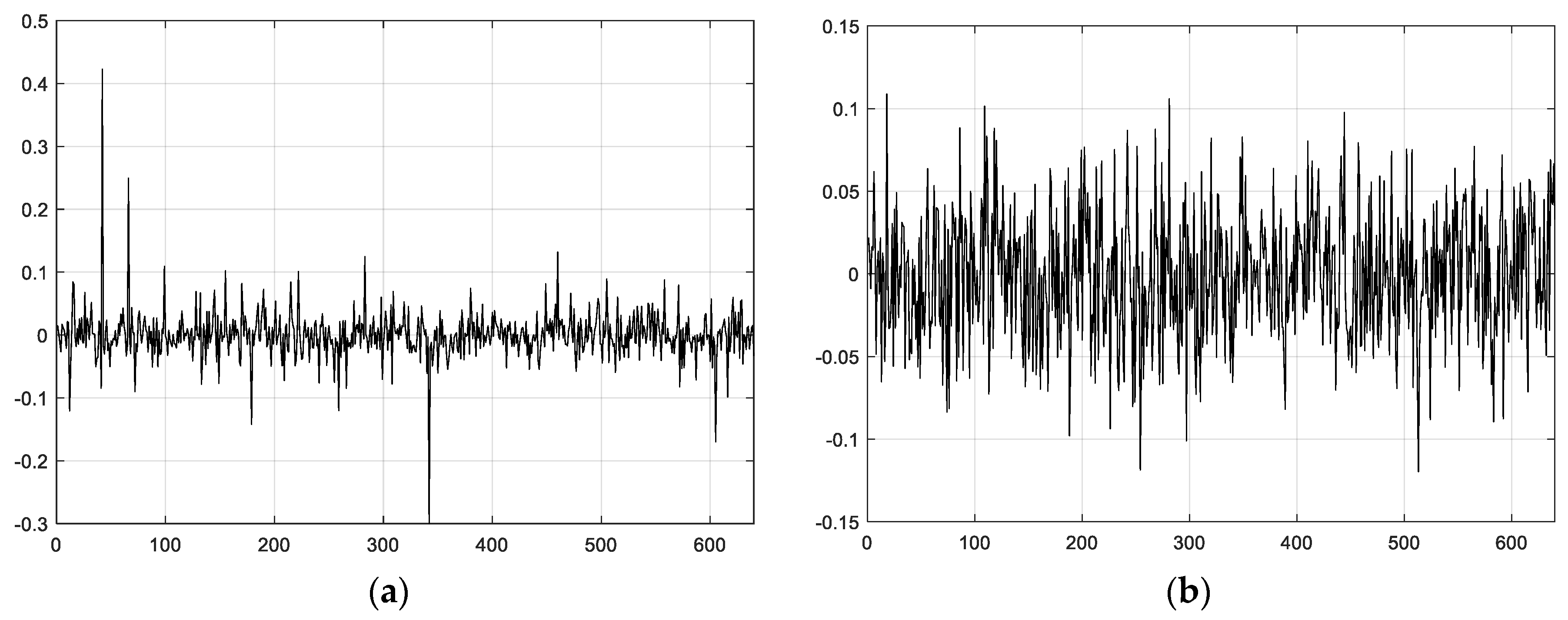
Figure 3 denotes the topology of 640 nodes of WSNs, and also represents some scale functions. To visualize the wavelets’ function, we plot
Figure 5 and
Figure 6 using the first scheme (Equation (12)) and the second scheme (Equation (13)), respectively.
Figure 5a introduces the second-level wavelet function, while
Figure 5b is the 10th-level wavelet function for the former schedule.
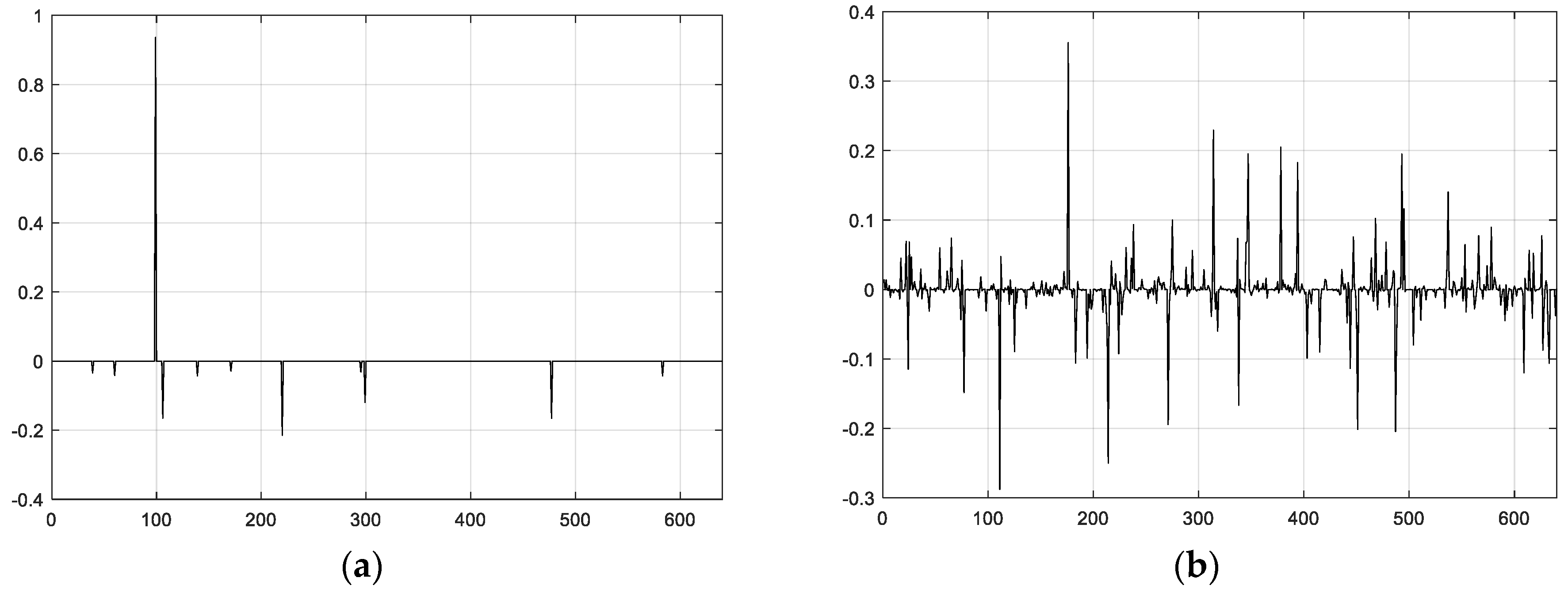
Figure 6 represents the second schedule considering the spatial correlation of sensor node readings in WSNs.
Figure 6a,b indicate first- and 10th-level wavelet functions, respectively. Obviously, the second scheme is set up on a sparser basis, for it can capture the sensor node’s relationship and network topology properties and thus gain valuable information from the real world.
4.3. Modified Ant Colony Routing Algorithm
In this paper, in order to decrease the whole network transmission load and prolong the network lifetime, we provide a modified ant colony routing algorithm, where to speed up the convergence rate and avoid local optimal of the algorithm, pheromone impact factor is improved. Here, we select the energy consumption model described in
Section 3.2. The traditional ant colony optimization algorithm selects the next hop depending on Equation (15) [
39]:
where
denotes the pheromone information on edge
, while
is the heuristic information on edge
.
and
are impact factors demonstrating the importance degree of the pheromone information and heuristic information. In order to speed up the convergence rate and avoid local optimal, impact factor
is modified as in Equation (16):
where
is a small positive constant
;
and
refer to current iterations and total iterations, respectively. In Equation (16),
gradually becomes smaller as the number of iterations increases. In other words, the proportion of pheromones will diminish when the number of iterations rises.
Furthermore, to yield optimal routing by the ant colony algorithm, in this subsection, a sensor node’s residual energy and path length are taken into consideration simultaneously. So, the fitness value of each routing is presented as follows:
where
indicates the average residual energy, while
represents the node minimal energy of ants passing through the path.
denotes the reciprocal of path length for given
ant and
iterations.
and
are
constants, and
. Consequently, the path with the largest fitness function value is chosen as the optimal routing, thus balancing the network load and prolonging the network lifetime. Specifically, the modified ant colony algorithm is shown in Algorithm 2.
| Algorithm 2.
Modified ant colony algorithm. |
| Input:
the number of sensor nodes , the power expended to run the transmitter or receiver circuitry of sensor node , energy consumption of multi-path fading amplifier , energy consumption of free-space amplifier , distance threshold , impact factors of pheromone information , impact factors of heuristic information , is a small positive constant , pheromone information on edge , heuristic information on edge , and are constants. |
| Output: optimal routing . |
| 1 Initialization routing , energy for each node and tabu |
| 2 calculate distance of different nodes, |
| 3 while maximum iterations has not be reached |
| 4 for =1: |
| 5 compute according to the node communication radius. |
| 6 generate transition probability based on Equations (15) and (16) |
| 7 choose the next hop node, relying on , modify routing and tabu |
| 8 the destination node or not? If not, go back to step 2, or proceed to step 9 |
| 9 update the node residual energy based on Equations (5) and (6), routing depending on Equation (17) |
| 10 end for |
| 11 end while |
| 12 return the optimal routing . |
4.4. Compressive Data Gathering
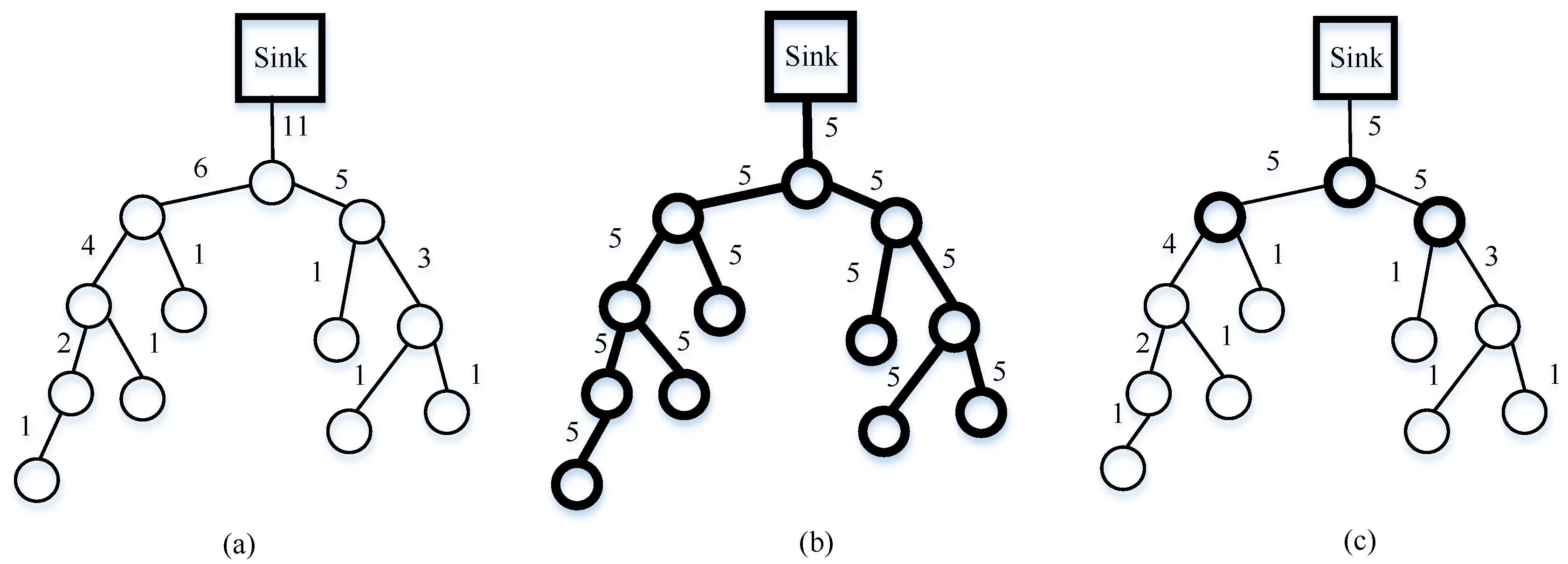
WSNs are utilized for gathering physical signal from the real world in practical applications. Without using CS theory, which is the simplest method, a data-gathering scheme with the help of the tree topology is shown in
Figure 7a. In order to dramatically decrease communication costs and prolong the network lifetime, the authors of [
12] consider that the sink node receives only
packets instead of
packets of original data from the whole network. In the end, at the sink, CS theory is used to reconstruct the original data. For the CDG algorithm, each node in the WSN multiplies its readings
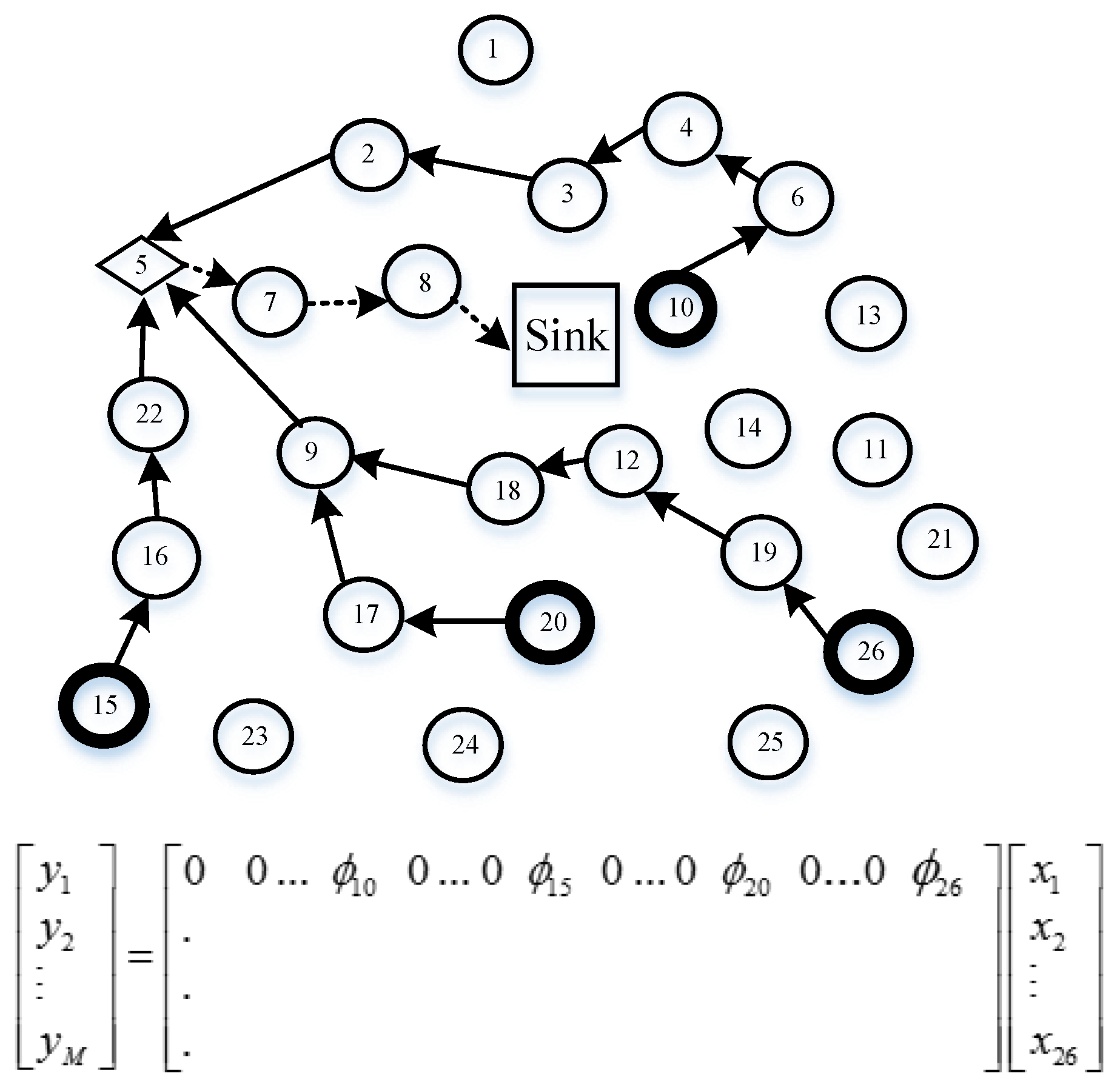
using the corresponding
column vector of basis matrix
. Next, the sensor node adds them to its own readings after receiving all same-size vectors from descendent nodes and transmitting the final results to its parent node with
packets. Let us illustrate the product of CDG in
Figure 8, where
is
matrix, and each column corresponds to one weight sum. In the plain CS [
11], all nodes in WSNs transmit
packets and each has equal transmission costs; therefore, each CS measurement cost remains relatively high. An example of the plain CS mechanism is given in
Figure 7b. It is obvious that for these approaches (non-CS and plain CS), the former transmits fewer packets compared with plain CS from the point of view of child nodes. In [
14], Wu et al. provides the hybrid CS method, where non-CS is chosen when the number of packets is less than or equal to
; alternatively, plain CS is used.
Figure 7c illustrates the idea of hybrid CS. In
Figure 7c, thin circles indicate a forward node using non-CS, while thick circles denote the gathering node using plain CS.
4.6. A Novel Data-Gathering Scheme with Joint Routing and CS
Obviously, according to the analysis, the network load in hybrid CS is unbalanced. Specifically, sensor nodes near the sink node will consume more energy than those far from the sink node because of forwarding data more times. This results in sensor nodes near the sink dying earlier. However, [
23] does not consider the total network costs for each random projection. To avoid the drawbacks, one can leverage the advantages of the algorithms; in this section, we present our data-gathering strategy combining joint routing and CS.
Firstly, randomly choose
projection nodes in the network with probability
, which follows [
23]. In the CS theory, the sink node needs
measurements to reconstruct the original data. Therefore, these
projection nodes will be selected as the gathering node, defined as
, to collect one random measurement
, and transmit
to the sink node. Then, distribute non-zero elements in each row of measurement matrix
as uniformly as possible to guarantee the sparse features of the measurement matrix; the number of non-zero elements in each row should equal to
, which is related to Algorithm 3’s step 1. Additionally, each column of measurement matrix represents a sensor node, so if a column of the matrix has full zero elements, the data from its special sensor node should be thrown away.
, the column vector of measurement matrix
is required to store each sensor node memory in advance. Now, an example of measurement matrix is given in Equation (18), where
, and
.
Secondly, each row
of measurement matrix
corresponds to one projection node. However, the number of each row coefficient is
, which is assigned to the size of network.
indicates that
candidate nodes belong to the
projection node’s. Here, this subsection corresponds to step 3 in Algorithm 3.
Subsequently, we set up the routing, which is from the offspring sensor nodes to the projection nodes and the projection nodes to the sink node, respectively. Based on the MST algorithm, access all candidate sensor nodes of a given projection node. In the first stage, the projection node is considered one root node tree. In the step 4 initialization stage in Algorithm 3,
is assigned by
i, and the temporary variable
also yields
. Then steps 5–12 use the MST algorithm to construct the tree, adding the candidate nodes step by step. If
is not empty, step 6 deletes the top node of the
queue and puts its neighbor node in the
and
. The next step is to delete them from
if they belong to
. Note that these candidate nodes must be directly connected to the parent node by a single hop. If there are still some candidate nodes not involved in the tree, the
algorithm [
40] is proposed, aiming to find the shortest path from the residual nodes to the tree (steps 14–19), and we add the residual candidate nodes (steps 20–22).
Finally, this loop of 13–26 lines will repeat until is empty. The modified ant colony routing technique is utilized to transmit packets of projection nodes to the sink node, namely step 27 of Algorithm 3. Consequently, Algorithm 3 terminates by generating the optimal routing between the projection nodes and the sink node, and an routing tree from the projection nodes to their own candidate nodes. Our novel algorithm (Algorithm 3) is shown in more detail. The modified ant colony algorithm jointly considers the sensor node’s residual energy and the path length, which will not only balance the whole network load, avoiding nodes near the sink node dying earlier, but will prolong the network lifetime. In this way, the transmission costs should be greatly decreased compared to hybrid CS.
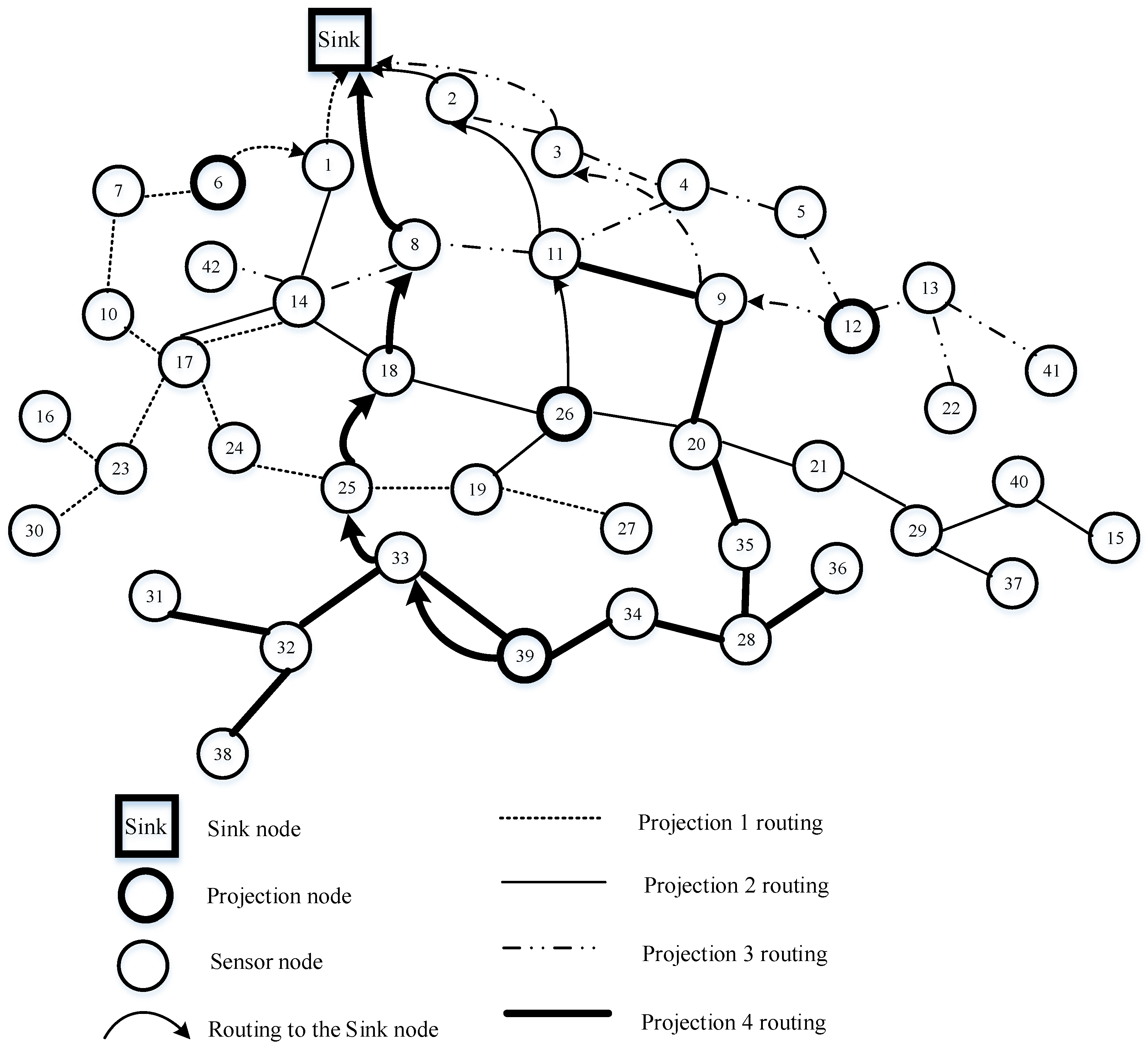
Figure 10 is taken as an example to describe the details of Algorithm 3. It can be seen from
Figure 10 that the thick circle indicates a projection node, the thin circle is a sensor node, the arc with an arrow represents the routing from the projection node to the sink node, and the dashed line, solid line, dotted and dashed line, and thick line describe four different projection routings. Sensor nodes 6, 12, 26, and 39 are chosen as projection nodes in the networks. Suppose that node 39 is the projection node in projection 4 routing, which has non-zero coefficients 9, 11, 20, 28, 31, 32, 33, 34, 35, 38, 39 of row vector
in the measurement matrix. Here, projection node 39 wants to establish a tree using Algorithm 3. Above all, node 39 considers itself a tree with only one node. Select its neighbor nodes 33 and 34, which can be directly coupled with node 39 by a single hop in the following step. Next, node 33 retrieves candidate node 32 as its neighbor node, so node 32 is added to the tree, while node 34 finds node 28 is also its neighbor node; similarly, node 28 is involved in the tree. However, in the coming stage, there are no candidate nodes directly connected with the tree. Therefore, the
algorithm is utilized to find the shortest path from the residual candidate nodes to the generated tree. Then nodes 31 and 38 are all joined to the tree, and nodes 35 and 36 are linked to node 28 by the shortest path. Again, nodes 20, 9, and 11 are involved in the tree using the MST algorithm. Finally, node 39 queries an optimal routing to the sink node for the projection node 39, which is
, rather than
using the
algorithm. The reason is that the modified ant colony chooses the next hop considering not only residual energy but also path length. So, node 33 chooses node 25, which has more residual energy compared with node 19. The same reasoning is applied to node 25 and node 18. Node 1 near the sink node forwards data many times from the other nodes, leading to considerable energy reduction. Therefore, in order to ease the burden on the network, node 8 chooses a direct path to the sink node, instead of node 1, although node 1 is actually the shortest path. Similarly, the routing constructed in projections 1, 2, and 3 is shown in
Figure 10. At the sink node, sensor signal reconstruction is implemented by Algorithm 4. In the process of the sensor signal, the gOMP [
28] recovery algorithm is utilized, where
denotes residual error,
is iteration.
represents the null set,
is
of
.
denotes the sets of indexes of
iteration.
| Algorithm 3. Our proposed algorithm. |
| Input: |
| Output: , |
| 1 randomly select sensor nodes in the network probability , generate |
| 2 for |
| 3 query candidate nodes () of projection nodes |
| 4 initialization , |
| 5 while !empty(temp) do |
| 6 |
| 7 if is ’s candidate node |
| 8 |
| 9 |
| 10 |
| 11 end if |
| 12 end while |
| 13 while !empty() do |
| 14 for all residual candidate nodes |
| 15 find a shortest path to using the algorithm |
| 16 if > |
| 17 |
| 18 end if |
| 19 end for |
| 20 |
| 21 |
| 22 |
| 23 while !empty(temp) do |
| 24 go back to steps 7–11 |
| 25 end while |
| 26 end while |
| 27 Optimal routing from to the sink node using Algorithm 2 |
| 28 return |
| 29 end for |
| Algorithm 4.
Sensor signal reconstruction. |
| 1
Input: received data , measurement matrix , the number of atom is |
| 2 Output: reconstruct data |
| 3 generate sparse basis using Algorithm 1 |
| 4 collect data in the network using Algorithm 3 |
| 5 |
| 6 initialization residual error , , , |
| 7 compute , select the largest values from ; these values correspond to ’s column indexes , constructing set |
| 8 set , (for all ) |
| 9 |
| 10 update |
| 11 , if go back to step 7, or proceed to step 12 |
| 12 reconstruct , which is the generation value of the last iteration . |


