2.1. Design of Road Watch Module
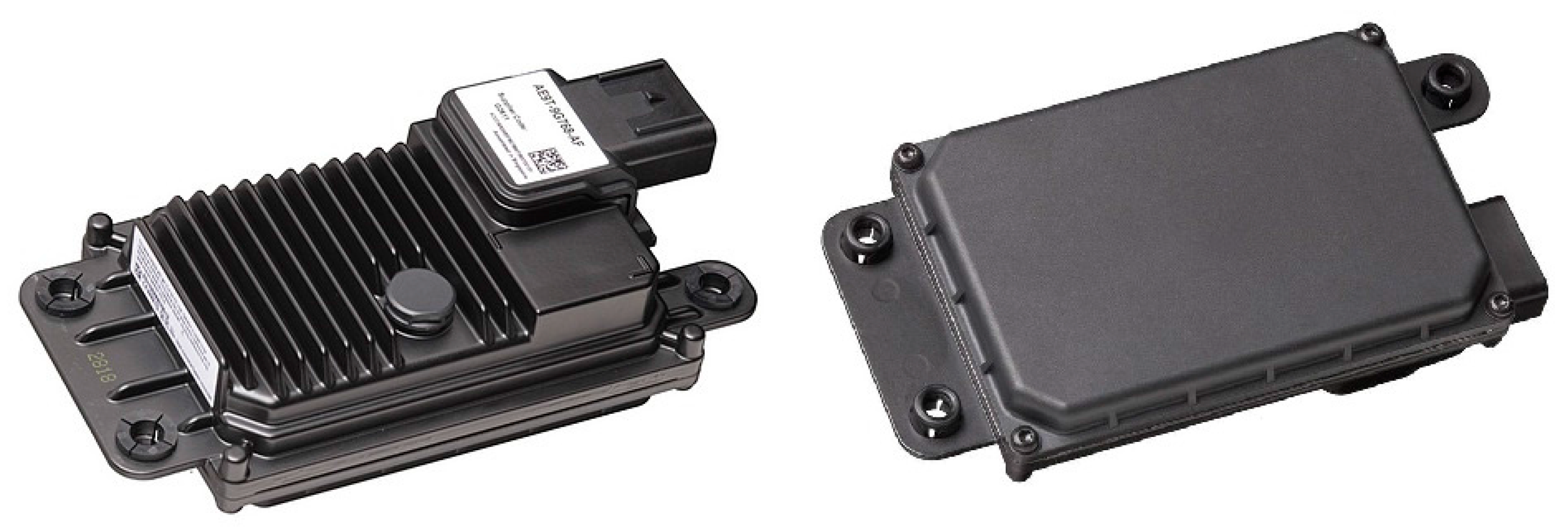
For accurate and stable vehicle traffic analysis on the roadside, the radar sensor is commonly used as the main detection equipment around the world. The type of radar varies according to the frequency band and the modulation method. Among the various radar sensors, however, we design an efficient deployment method for optimal detection performance on the road by using Delphi’s ESR radar [
23], which is currently one of most popular products for vehicle detection and has excellent price competitiveness. The radar platform and detailed specifications are shown in
Figure 1 and
Table 1, respectively.
In this study, a road watch module (RWM) based on ESR was designed. The main purpose of this module is to detect stationary and moving vehicles within the detection range of the radar sensor provided by the radio frequency (RF) signal of an antenna device. It also detects the position, lane, and speed information of the target vehicle. The vehicle to be monitored and the target road environment are selected as follows. The width of the vehicle is selected to be 1–2.5 m in reference to the sedan and the recreational vehicle (RV), which are the most popular vehicles for general people. The number of lanes in the road is 2–4 with a width of 2.5–3 m. The radar platform is installed on the roadside and the installation height is set to 2.5–3 m, which is the average height of the roadside traffic sign. Meanwhile, this installation height is different with the case of automotive radar due to the fact that the installation height of the radar in the vehicle is 60 to 100 cm, which is the height of the vehicle bumper.
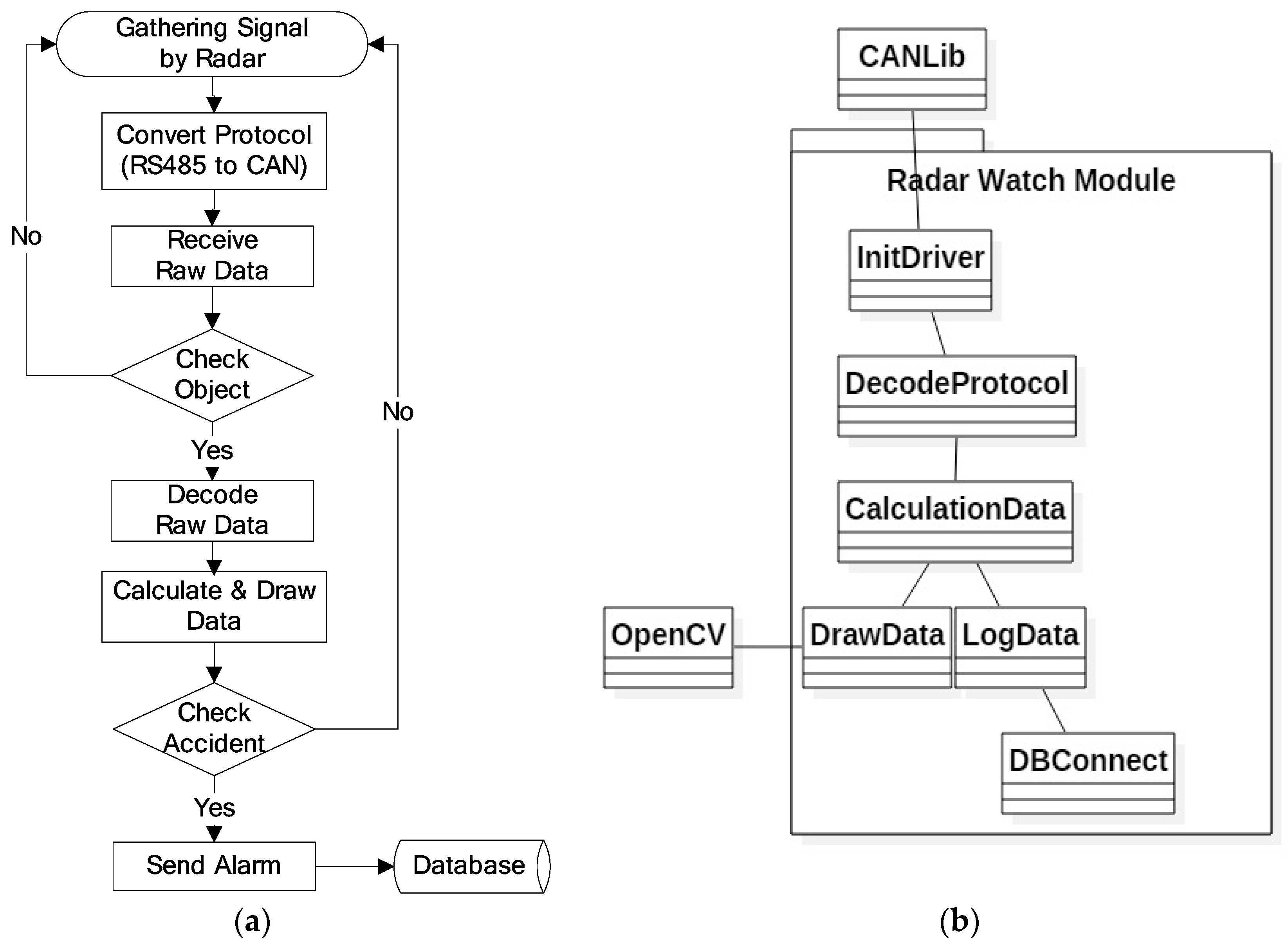
After the installation of the radar, the user application connected to the radar should interpret the detection data streams obtained from the RF, and the RWM performs the function of acquiring and decoding these detection data streams. For this, the RWM and the radar sensor communicate with each other based on the Controller Area Network (CAN) protocol [
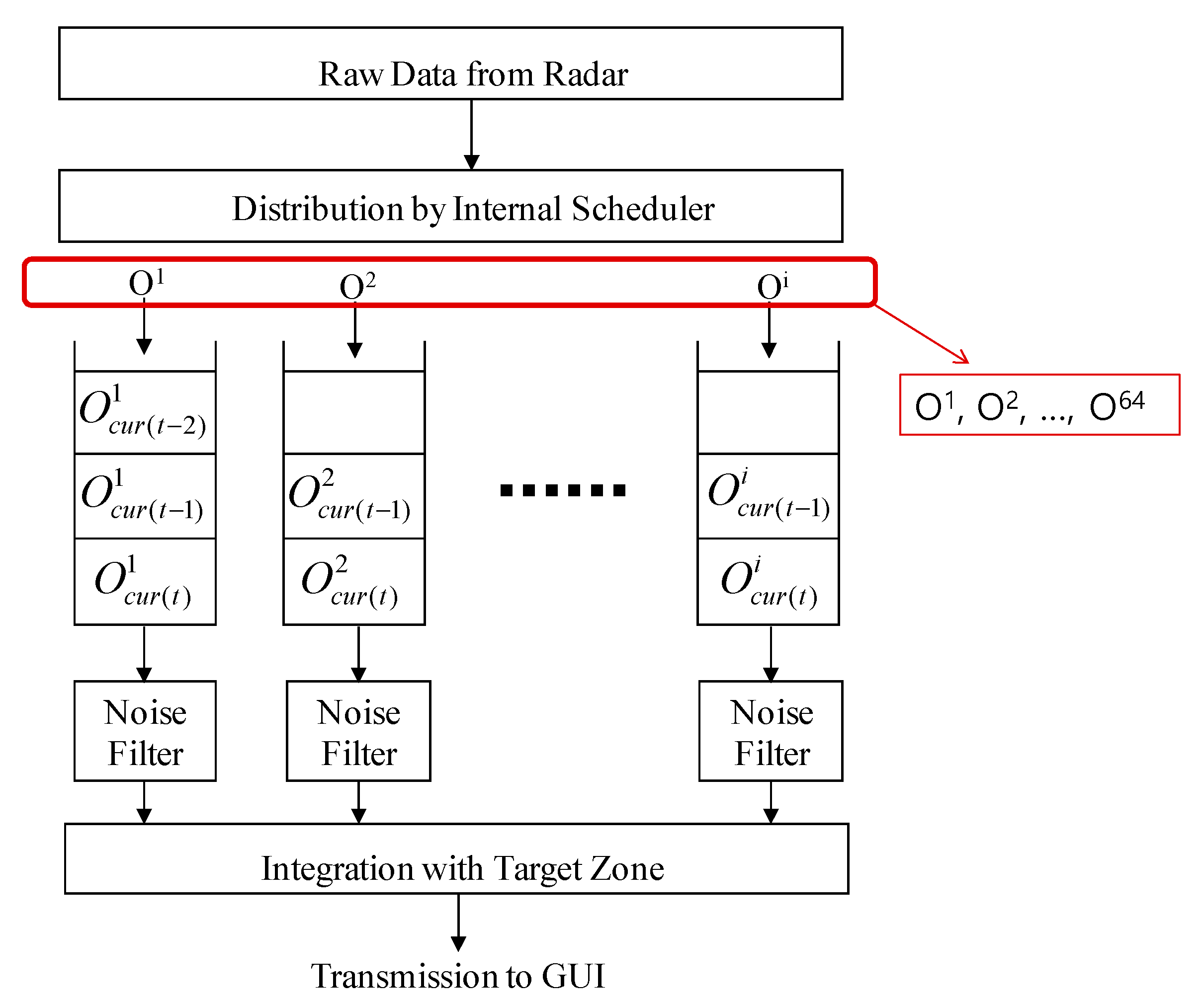
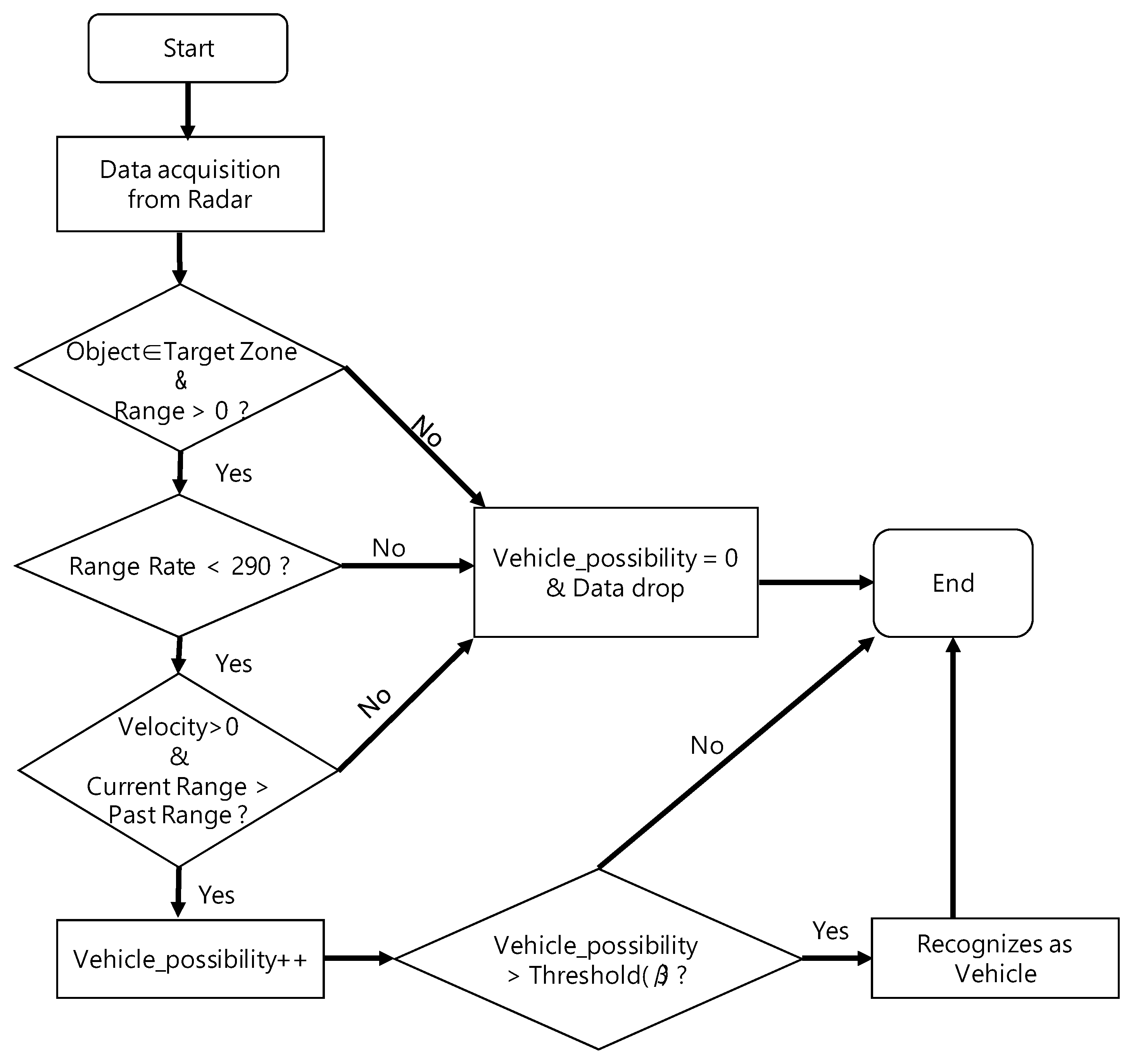
6], which transmits bit stream through the network interface. After decoding the data stream, RWM can distinguish stationary objects (e.g., buildings, trees, road signs) from moving vehicles by adopting a real-time speed comparison algorithm. In addition, it also maintains a text log component that stores a raw data stream in real-time, so that it is possible to confirm that the RWM successfully receives every data stream provided at an update rate of 50 ms. The detailed operation sequence and module diagram are shown in
Figure 2a,b respectively.
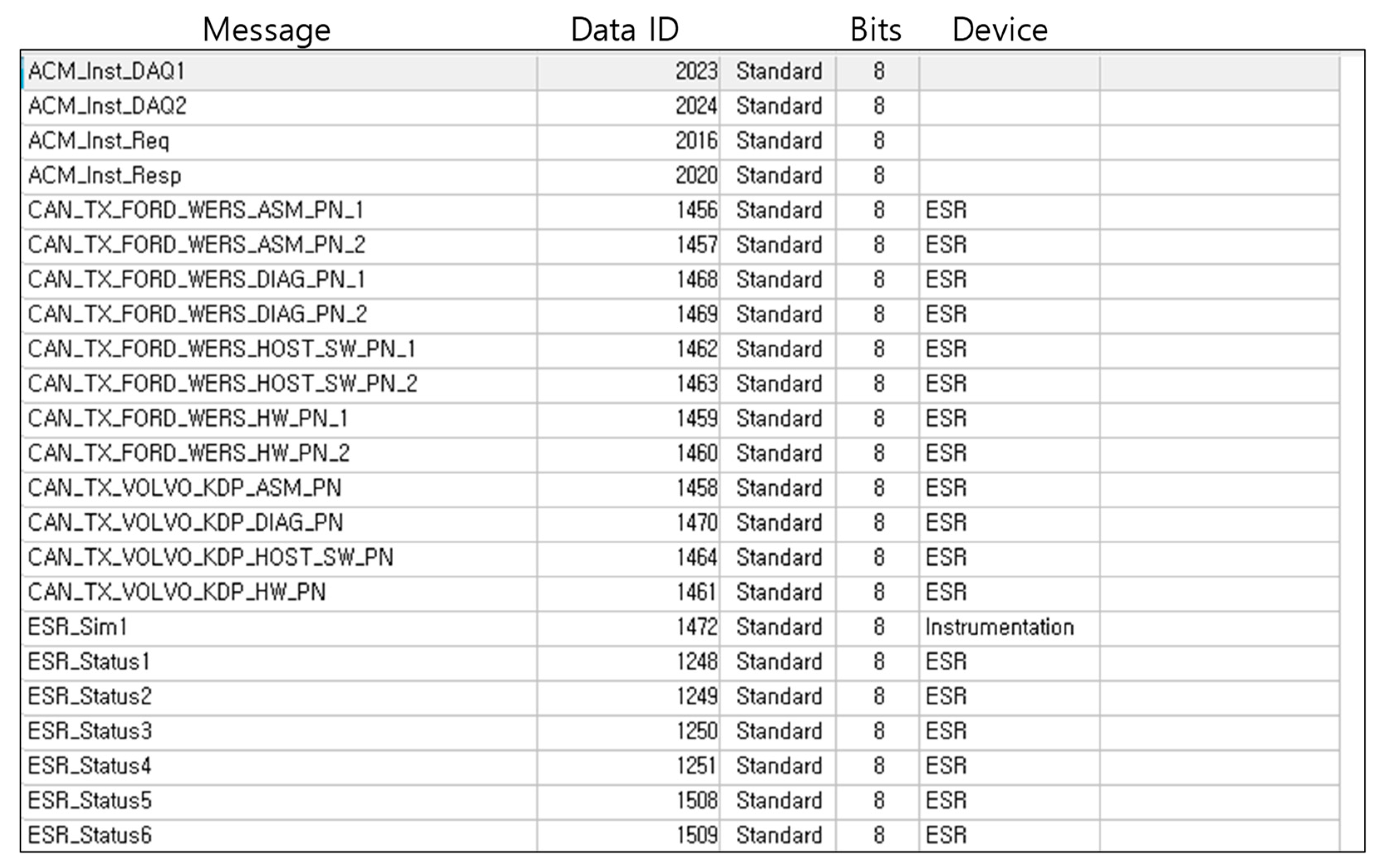
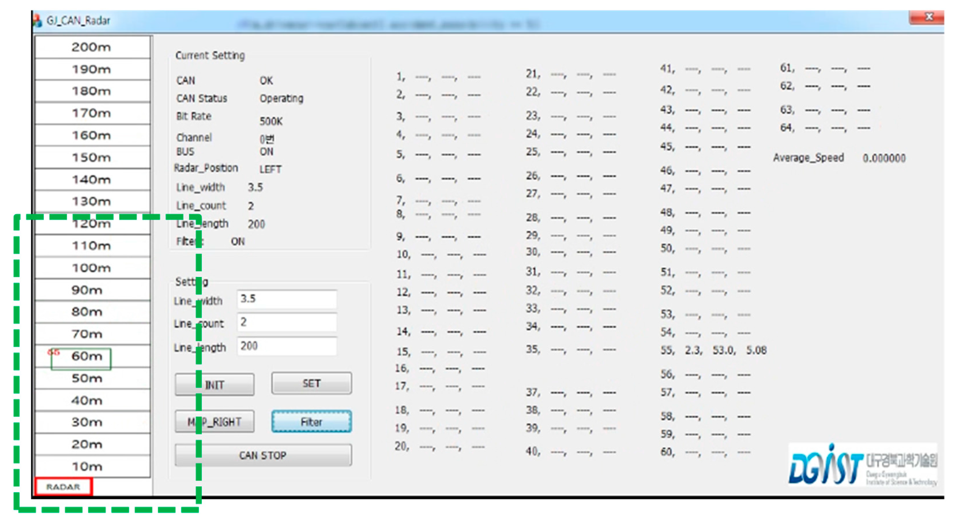
The overall operation flow of the RWM is a series of functional iterations which are performed in the following order: radar signal collection, protocol conversion, raw data reception, object identification (ID grant), raw data decryption, data calculation, accident check (e.g., abnormal vehicle detection), abnormal signal notification and database storage. In the radar information collection function, RWM collects a data stream including the distance, speed, and length of the object detected by the radar. In protocol conversion, the RWM converts the incoming radar data provided by the RS485 communication protocol into the controller area network (CAN) protocol. The “raw data reception” component receives and inserts the raw data, which is then delivered by the CAN interface into the RWM buffer. In the “object identification” component, the RWM assigns a unique ID to an object identified as a detected target among the received raw data. That is, the object to which the ID is assigned becomes a moving vehicle or an obstacle (clutter) to be monitored. If the data is not judged to be a target object (e.g., radar management data) to be monitored, it moves to the radar signal collection section and then it repeats the signal collection process. The example information that is excluded from the set of monitoring objects is shown in
Figure 3, where the representative one is digital to analog (D/A) converted information, data acquisition (DAQ) related information, device diagnosis related information and so forth. For more detailed information on radar data, please refer to the Kvaser database [
24].
The main advantages of the proposed RWM are summarized as follows:
- (1)
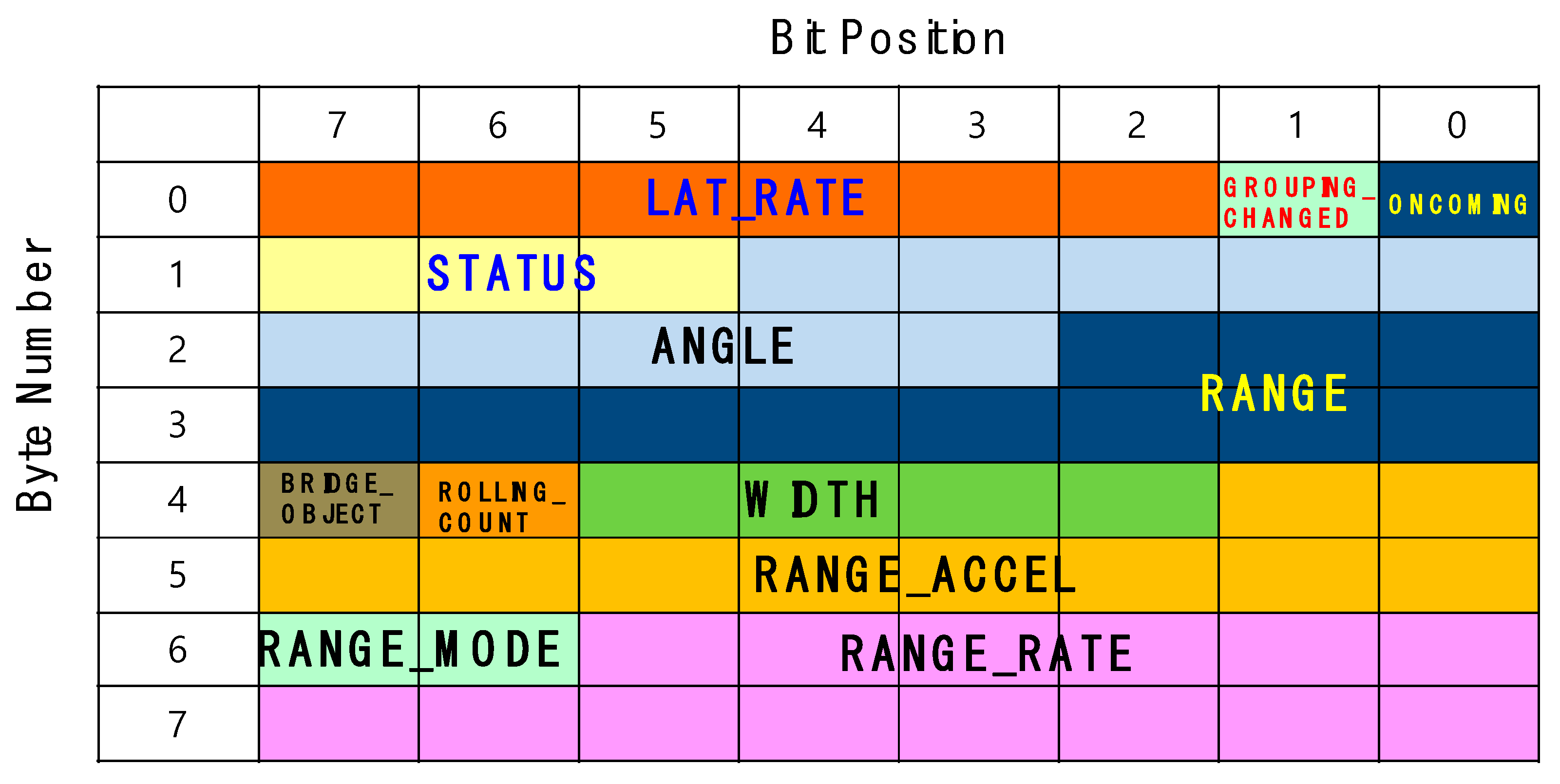
Generally, the objects’ information that is obtained from the radar is very diverse and the amount of information is also very large. This large amount of data is still a burden to process in real-time on embedded devices connected to the radar. For this purpose, RWM preferentially inputs only those attributes that are relevant to the moving vehicles, minimizing the response latency by filtering meaningless information. In particular, since Delphi ESR radar only provides bitmap information of raw data, as shown in
Figure 4, and does not provide data selection, acquisition, or communication methods for specific applications, the RWM provides a framework for the analysis and processing of the raw data from the radar.
- (2)
With respect to the vehicle information obtained, only the vehicle located in the road is tracked with reference to the width of the road, the number of lanes and the length of the lane, so that the processing delay time can be reduced and detection accuracy can be enhanced.
- (3)
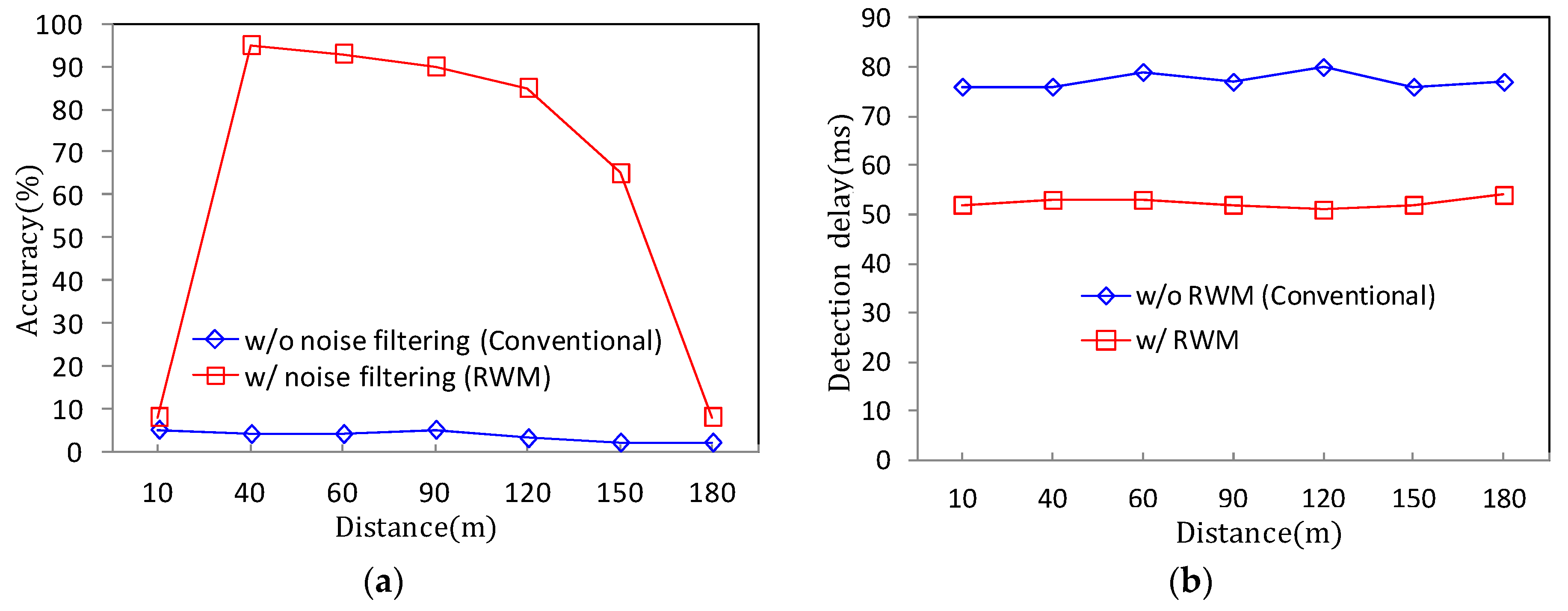
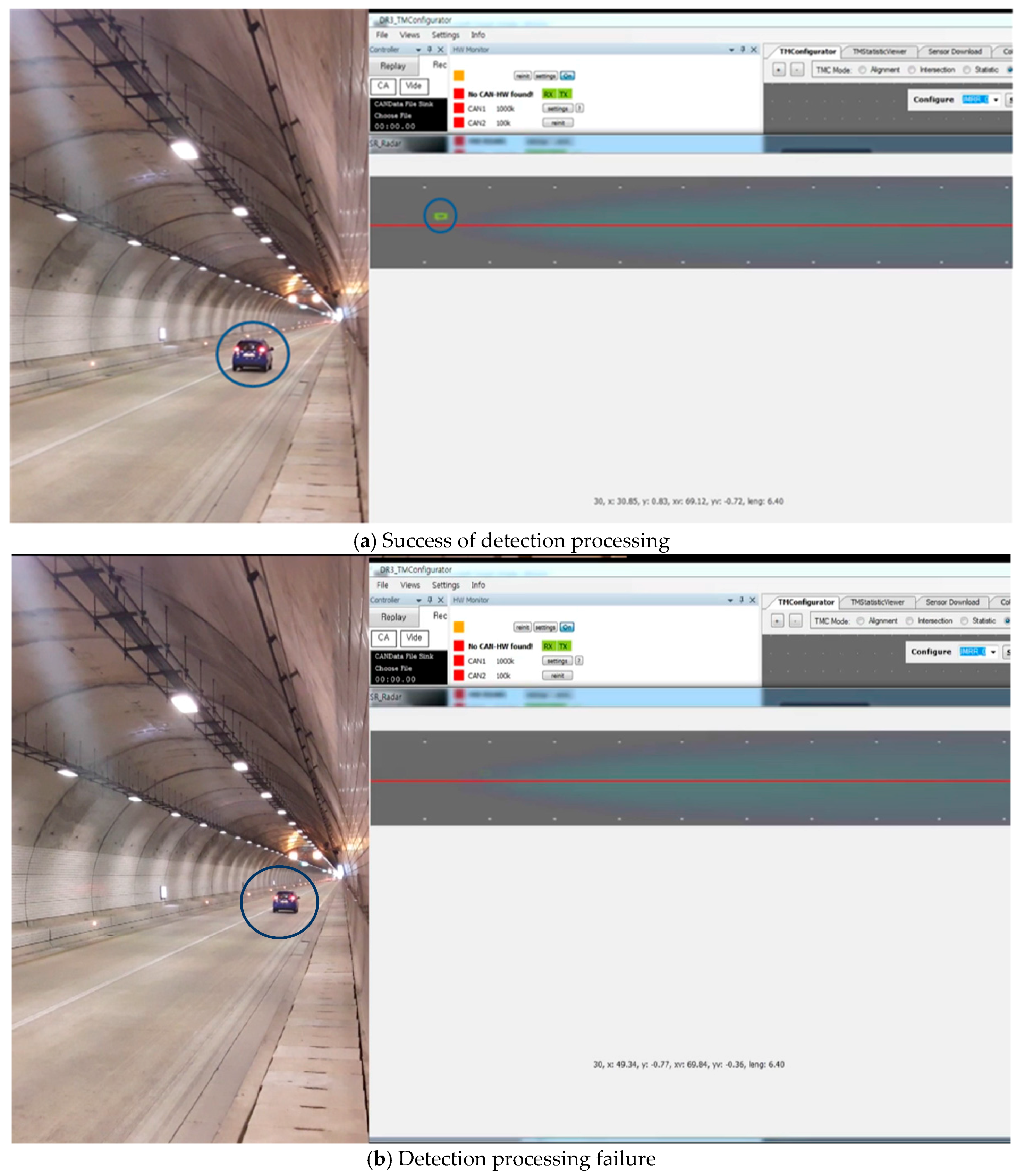
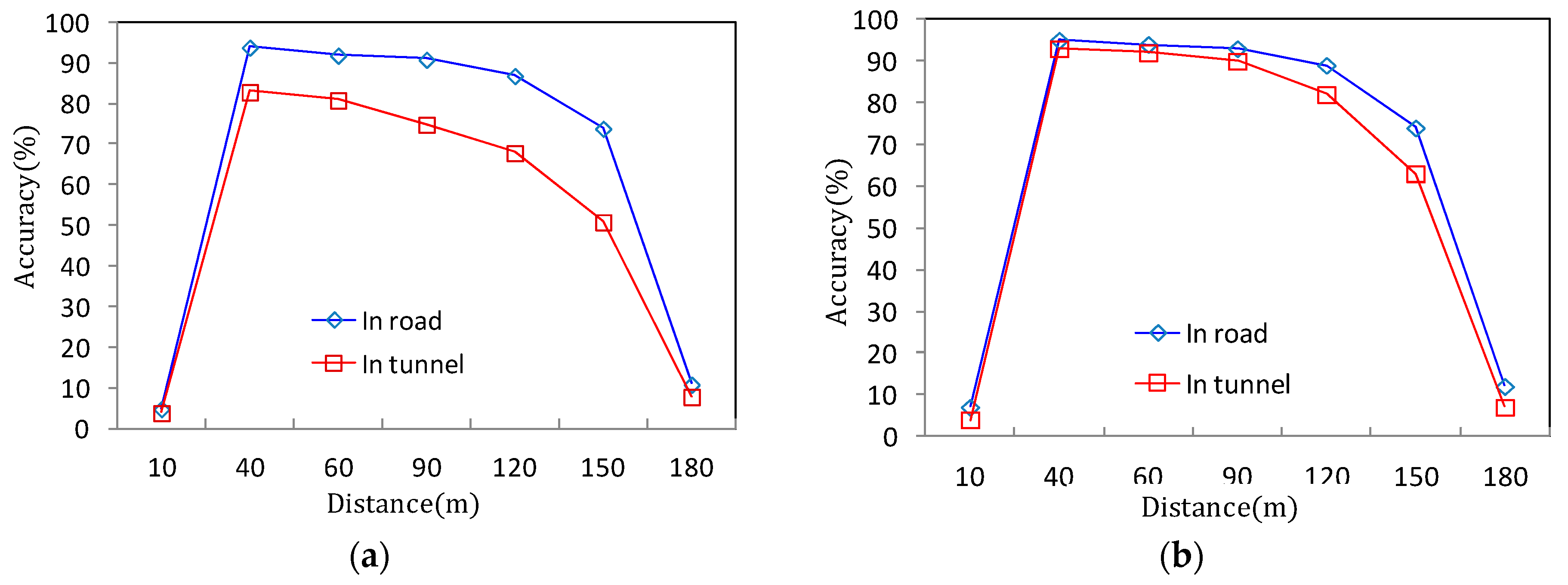
In addition to accurate vehicle identification on the road, the RWM also provides a noise filtering technique in tunnels by analyzing various false signal patterns such as ghost phenomena and flickering. The proposed scheme provides robust detection accuracy and low calculation latency in tunnels.
- (4)
By adopting the RWM technique, it is possible to confirm the occurrence of an accident by analyzing the stop pattern and congestion phenomenon of a vehicle.
In the “raw data decoding” component, the RWM application extracts necessary information by decrypting the raw data stream. That is, the meaningless raw data acquired from the radar is converted into high level information which is utilized at the application level. A bit-map of the data protocol used for decoding is shown in
Figure 4.
The above bitmap is composed of 8 bytes and the information about the target vehicle’s motion such as the speed, direction, and distance is as follows:
- −
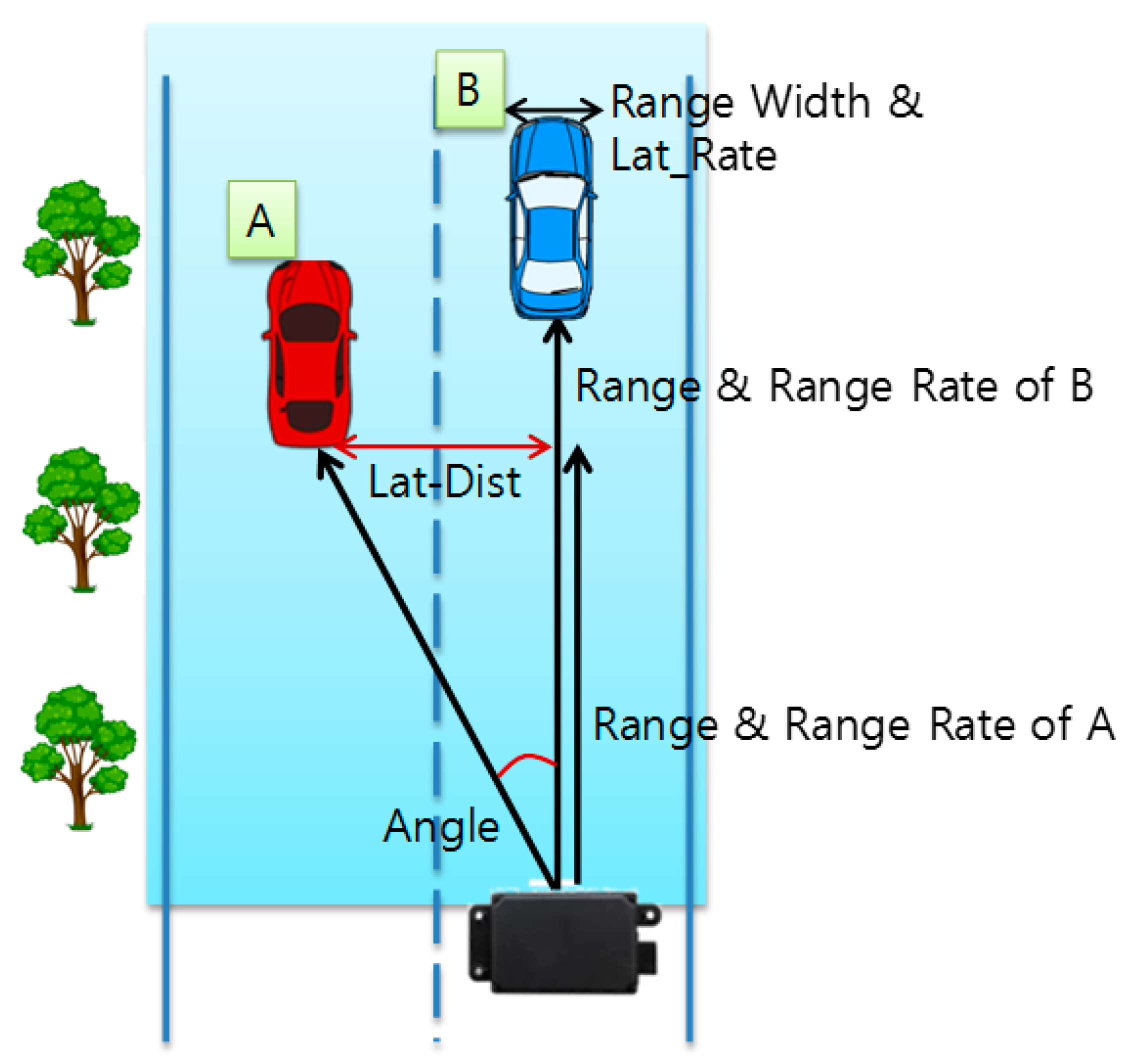
ANGLE: Angle of the RF signal that is reflected from the target object after the radar transmits it.
- −
LAT_RATE: Speed of an object moving in the horizontal direction between lanes.
- −
RANGE: Distance between the radar and the target object.
- −
RANGE_RATE: Relative speed between the radar and target object.
- −
RANGE_WIDTH: Width of the target object.
Figure 5 shows an example of the measurement of the moving vehicle on the road using the extracted information via the RWM. In
Figure 4, if the radar is installed in the middle of the road or the radar is mounted on the front bumper of the vehicle, the vertical distance between the preceding vehicles A and B, the relative speed between radar and vehicles and the angle with respect to the forwarding direction can be known. However, since the ESR radar is mainly concerned with the presence or absence of the front obstacle according to adaptive cruise control (ACC) or advanced emergency brake (AEB) operations, the horizontal distance between lanes for vehicle A is not explicitly provided. Nevertheless, because ANGLE values can be checked, we can easily find Lat-Dist by using the following equation:
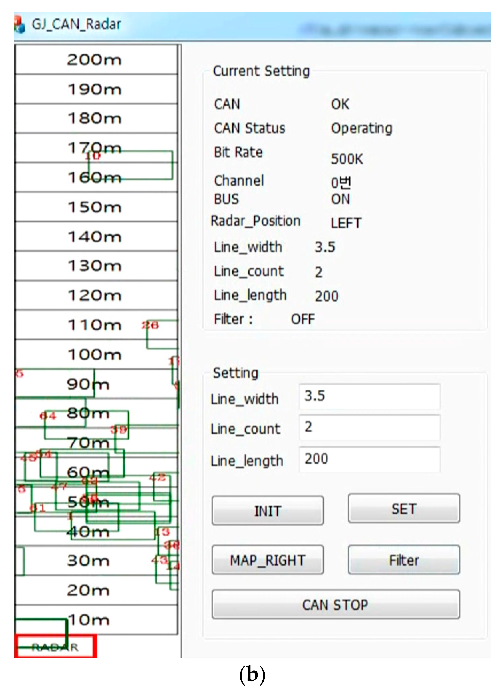
The “calculate & draw” component has the role of verifying whether the detected object is located in the current lane or road, based on the coordinate information obtained through Equation (1) and the information on the physical environment of the road. After finishing the verification of the target object, it also provides a function of displaying corresponding object information in the graphical user interface (GUI). For this, the user can first input the information of the target road on which the radar is installed. As shown in
Figure 5, three pieces of environmental information (such as the width of the road, length of road and the number of lanes) to be monitored are set through the main GUI provided by the RWM. However, the length of road, which is measured and displayed, does not exceed the maximum monitoring distance (Range_Max) of the radar. In the case of Delphi ESR radar, Range_Max is defined as 174 m. Through the three pieces of input information, we can set the target zone to be monitored by the radar, and it is easily calculated with the following equation,
where, LW, LC, and LL denote the lane width, lane count and lane length of the target road, respectively. The calculated target zone is within the range of the blue rectangle in
Figure 4. In addition, by tracking only moving objects within this range, it is possible to improve the calculation speed and increase the recognition rate of the vehicle by excluding the reception of unnecessary clutter information such as trees, buildings, street lamps and so forth. In
Figure 4, the objects recognized as vehicles in the range of the radar are displayed in square form through the OpenCV library [
25] on the target zone. Vehicle A and Vehicle B in
Figure 4 are assigned ID 28 and ID 24 in
Figure 5, respectively, and they are shown in green squares. In addition, the Lat-Distance, Range, and Velocity for each vehicle are displayed in the ‘Radar Data’ field on the right side of the GUI for specific object movement information. The velocity is marked as ‘+’ when moving away from the installed Radar, and the approaching object is marked with ‘−’. In
Figure 5, the two vehicles—ID 24 and ID 28—are approaching at 79.85 km/h and 78.51 km/h, respectively. In the case of ID 24 in
Figure 5, the data set of [24, 2.9, 91.6, −79.85] denotes that the vehicle’s ID is 24, Lat-Distance is 2.9, Range is 91.6 and velocity is −79.85. At this time, it is important to note that the three trees shown in
Figure 5 are excluded from
Figure 6 because they are outside the target zone. Meanwhile, a complicated section where the radar cannot overcome a non-line of sight (NLOS) condition, such as a curved road or an intersection, can be monitored by overlapping a plurality of radars.
The “check accident” component provides a function that warns the user of a vehicle accident. Although there are many kinds of vehicle accidents, the main accident is defined as a case in which the vehicle is unexpectedly stopped on the road due to a collision or breakdown. To analyze the accident stop pattern, the RWM uses the following conditional equation,
Condition 1. Target_Zone
Condition 2. = 0, θ > 0
is the position of vehicle
i at current time
t. Condition 1 determines whether the vehicle is within the target zone of the radar.
represents the average speed of vehicle
i during the period from the current time
t to
t +
θ. Condition 2 confirms whether the vehicle is in a stopped state (i.e., velocity is 0 km/h) during the threshold time (
θ). In this study,
θ is set to 30 s although it depends on traffic conditions and traffic regulations on the target road. Of course, it can be set shorter on the road for the exclusive use of vehicles (e.g., expressway). If the vehicle is stopped for a certain period of time using the above two conditions, an accident may be suspected. However, if vehicles are backed up due to a road bottleneck phenomenon, the vehicle will inevitably be stopped. In this case, it is difficult to distinguish an accident from a bottleneck. To resolve this problem, we use Conditions 3–5 below.
If there is not a large-scale collision accident, it is regarded as a bottleneck. Since the bottleneck phenomenon means that all vehicles are stopped, this condition is expressed as Condition 3, as follows.
Condition 3. Generally, after a certain period of time, the preceding vehicles continue to move as the bottleneck is alleviated. At the same time, the i-th vehicle also starts to move at a higher speed to deviate from the area of interest. In this case, it is recognized as a normal traffic pattern or a simple bottleneck rather than an accident. On the other hand, although the preceding vehicle has started moving and has departed from the target zone, vehicle i is judged to be an accident vehicle if the vehicle i is kept in the stopped state for a critical time. In this situation, the movement of the preceding vehicle except for vehicle i is expressed by Condition 4.
Condition 4. where x is the time until the bottleneck disappears. The time can be measured in real-time via the vehicle’s flow in the radar or by manual input. The condition where vehicle i is stopped for the critical period after the bottleneck release point is expressed in Condition 5 as follows.
Condition 5. As a result, if the above five conditions are satisfied, the RWM confirms that a bottleneck phenomenon is not currently present, and transmits the coordinate information (Range, Lat-Distance) of vehicle i to the user along with an accident judgment message. After an accident alarm, the corresponding information is recorded in the database in the “DB storage” component.
2.2. Derivation of Optimal Performance for Roadside Deployment
In order to evaluate the performance of the developed RWM and to derive the optimum performance conditions, the vehicle detection accuracy was measured. The detection accuracy was calculated as the average of two accuracy results, which include the accuracy of a moving vehicle (Accuracy_MV) and the accuracy of a stopped vehicle (Accuracy_SV), assuming an accident. These measurement environments are expressed by Equations (3)–(5) as follows:
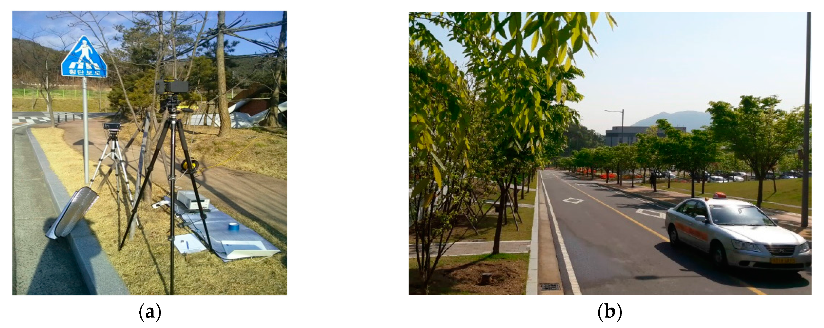
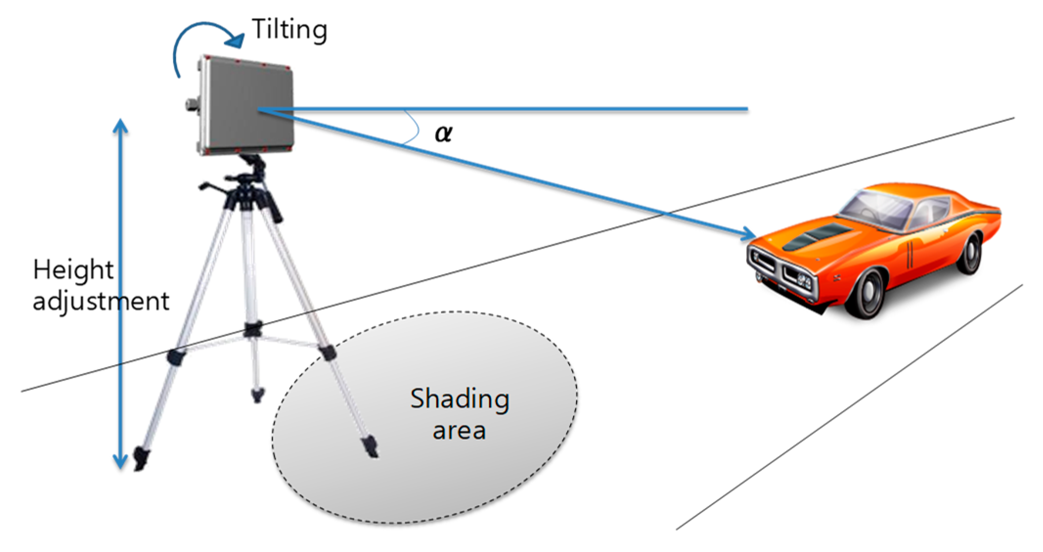
The target vehicles for the experiment were randomly selected on the campus road. For vehicle accident simulation, one sedan type vehicle was selected. To measure the detection accuracy, the selected vehicle was repeatedly run and stopped more than 50 times and the number of correct detections was measured. In order to increase the detection accuracy for the vehicles by installing the radar on the road surface, it is necessary to tilt it slightly in the forward direction of the road in consideration of the straightness of the RF signal of the radar. It is also necessary to set the high positioning of the radar for extending the detection range. Based on these facts, the vehicle radar is mounted on a dedicated cradle and placed on the roadside, as shown in
Figure 7. We then measured the detection accuracy while manually adjusting the height of the mount, the installation angle, and the number of target vehicles, as shown in
Figure 8.
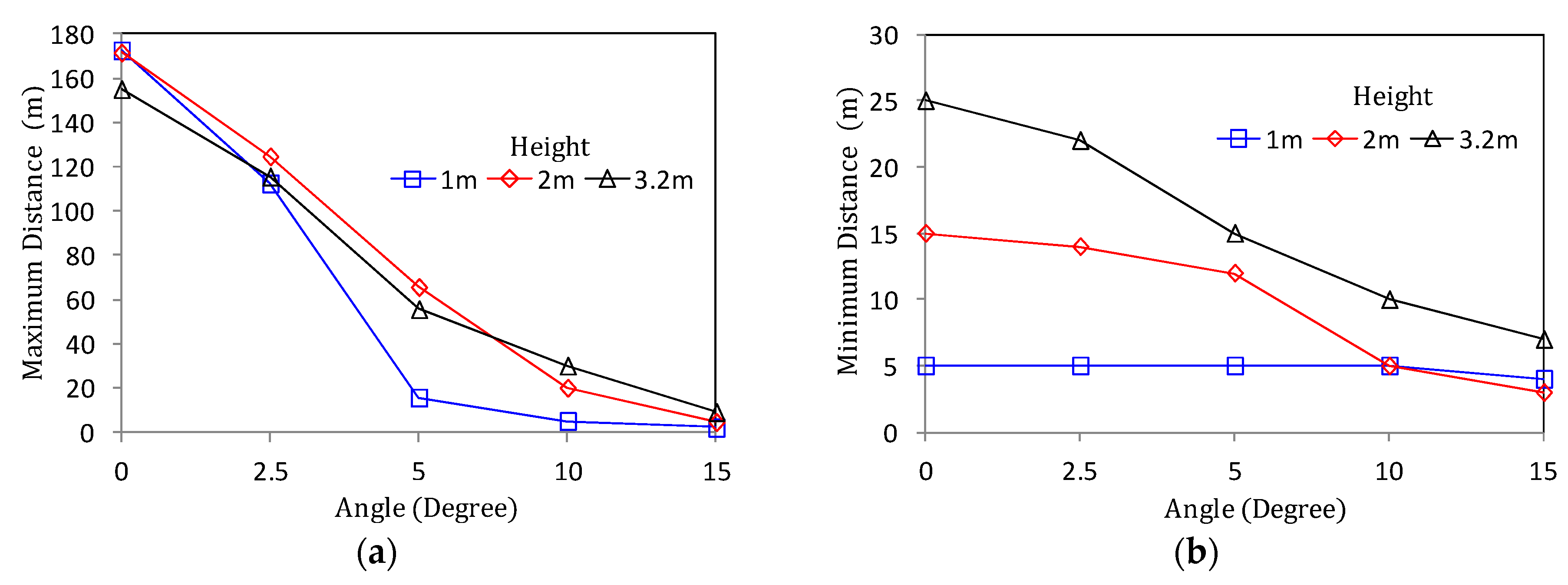
Prior to measuring the detection accuracy, we measure the maximum distance at which the vehicle is correctly detected according to the tilting angle α and the height of the radar installation, which is illustrated in
Figure 9a. In general, as the tilted angle becomes larger, the RF is directed towards the road surface, which means that the maximum distance to detect the vehicle becomes shorter. Especially, in the case of 1m height, the detection distance sharply falls when the angle is over 2.5°. Moreover, when the angle is greater than 5°, the detection distance is less than 20 m, which makes it difficult to monitor the traffic on the road. This means that the vertical field of view (FOV), in which an object can be recognized, sharply decreases.
On the other hand,
Figure 9b shows the minimum detectable distance based on the radar. It can be seen from the figure that the higher the installation height, the more signal shaded areas are generated below the radar where vehicle detection is impossible. In the case of 3.2 m and 2 m height, if the angle is 0°, the front shadow length of the radar is 25 m and 15 m, respectively. To overcome this long shadow area, it can be reduced by increasing the tilt angle. Whereas, in the case of 1 m height, the variation of the minimum detection distance is less than that of the angle adjustment. If only the detection distance comparisons of
Figure 9a,b are taken into consideration, then a low installation height and a low tilted angle can be accepted as reasonable installation conditions.
However, it is important to note that simply setting α lower than 2.5° does not always guarantee its performance.
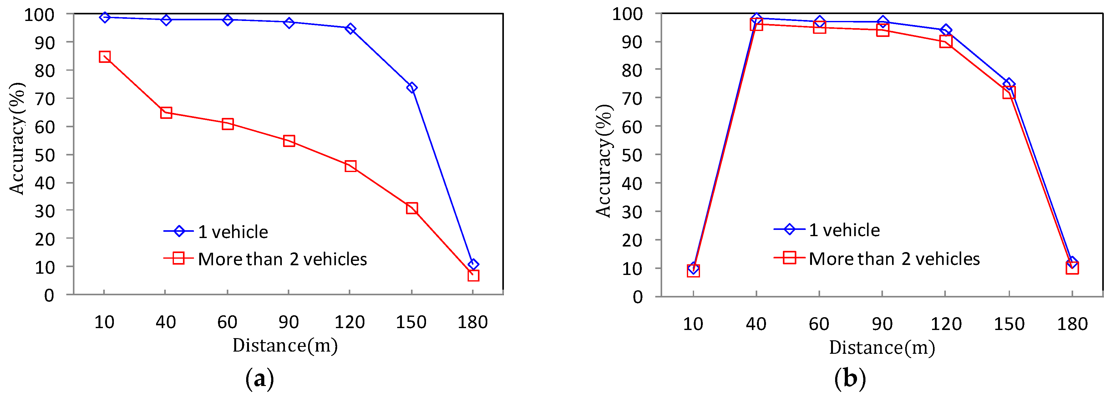
Figure 10a shows the detection accuracy of the RWM according to the number and distance of the monitored vehicles on the road at an installation height of 1 m. In the case of one target vehicle, the detection accuracy is more than 95%. However, when two or more vehicles are overlapped within the detection range of the radar, the performance sharply drops, and the average accuracy is approximately 60%. Since the height of 1 m is less than the actual height of the vehicle (i.e., averagely 1.5 m above the ground), the preceding vehicle is not detected by the radar due to the NLOS problem. That is, the preceding vehicle is hidden by the rear vehicle. As a result, the height of 1 m or less only can be adopted to the application of the ADAS system such as front obstacle detection or collision risk warning, but the performance is insufficient for road traffic monitoring on the roadside.
Meanwhile, in
Figure 10b, the same experiment is performed at a height of 2 m. The result reveals that even when two or more vehicles are moving, the recognition performance is not significantly decreased below that in the case where only one vehicle is moving. In addition, according to
Figure 9a, when the height is 2 m or 3.2 m, it is easy to reserve the wide vertical FOV. Therefore, the reduction of the detection distance performance by the tilting angle is relatively small compared to using a height of 1 m. However, because of the shadow area of around 15 m which is observed in
Figure 9b, the detection accuracy is also significantly decreased (less than 10%) within a 15 m distance. Of course, it can be seen that the performance of detection accuracy suddenly drops even when the maximum detection distance of 120 m derived from
Figure 9a is exceeded.
As a result, the experimental results of
Figure 9 and
Figure 10 show that the best performance, that is, the highest detection accuracy and the longest detection distance can be obtained when the radar is installed on the roadside with the tilted angle of around 2.5° at a mounting height of around 2 m.


