Spectral-Spatial Feature Extraction of Hyperspectral Images Based on Propagation Filter
Abstract
:1. Introduction
2. Proposed Method
2.1. Propagation Filter
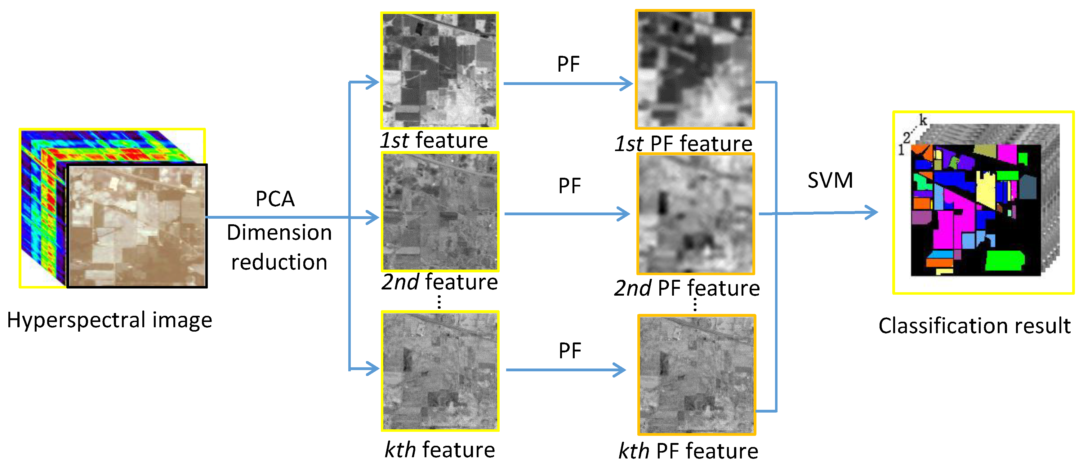
2.2. Spectral-Spatial Feature Extraction Method Based on the PF
| Algorithm 1: Specific flowchart of the spectral-spatial feature extraction algorithm based on the PF. |
 |
3. Experimental Settings
3.1. Dataset Description
3.2. Compared Algorithms
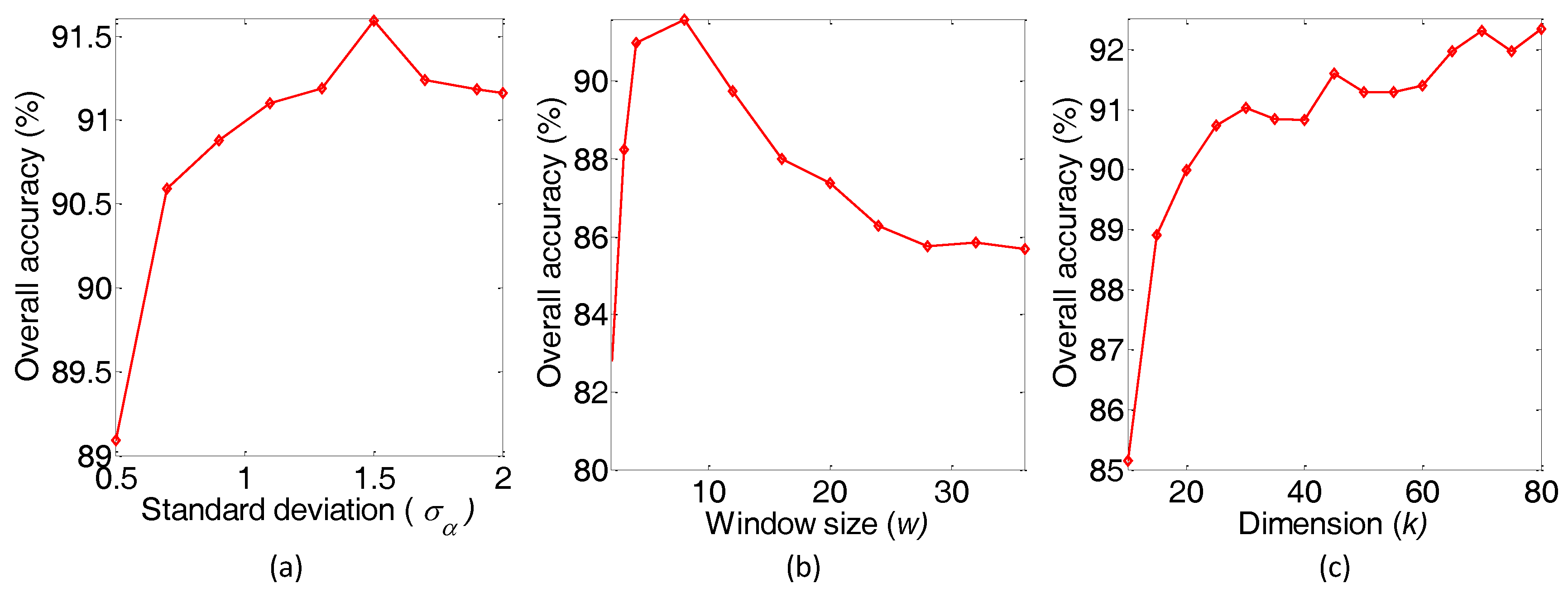
3.3. Parameter Sensitivity Analysis
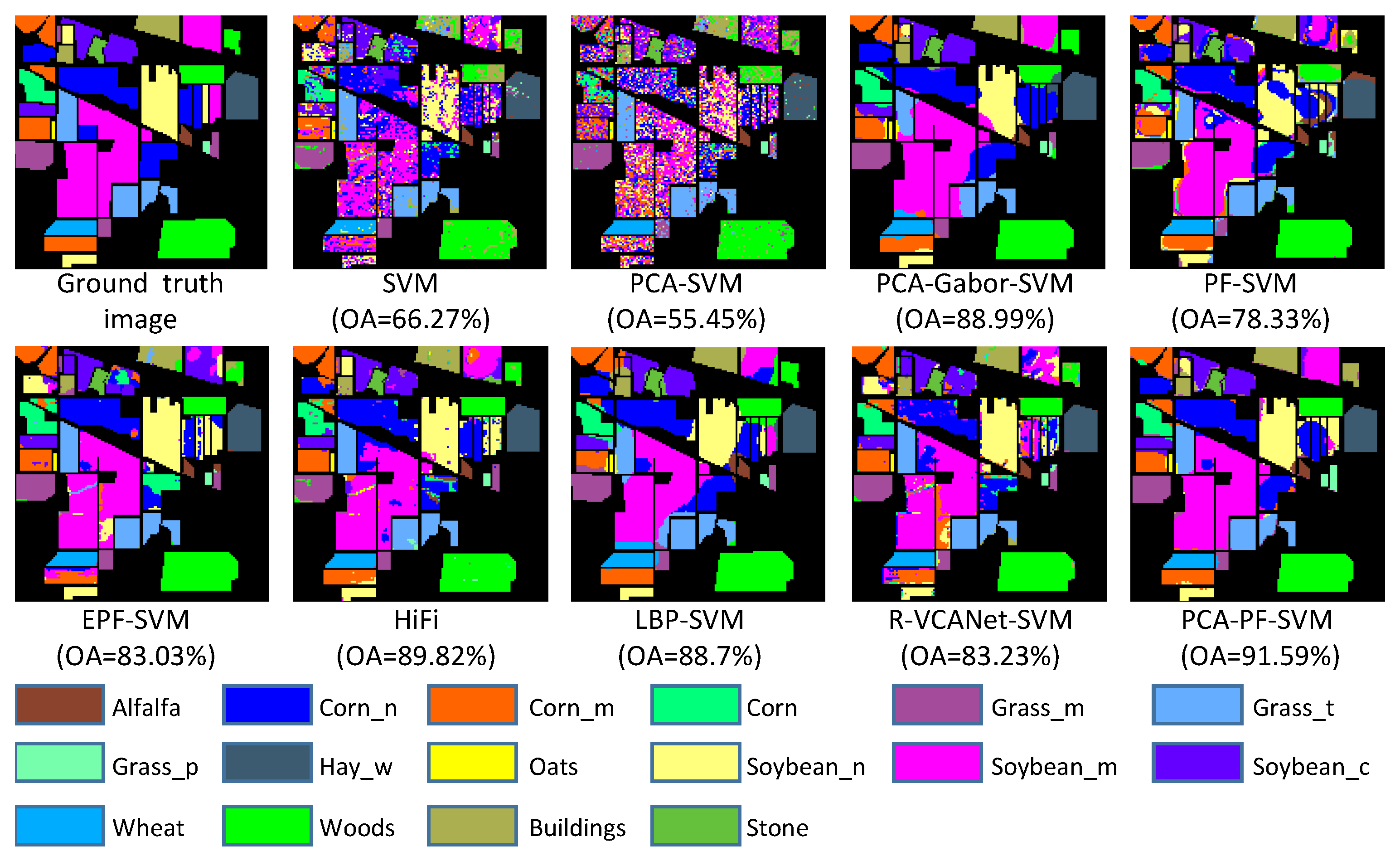
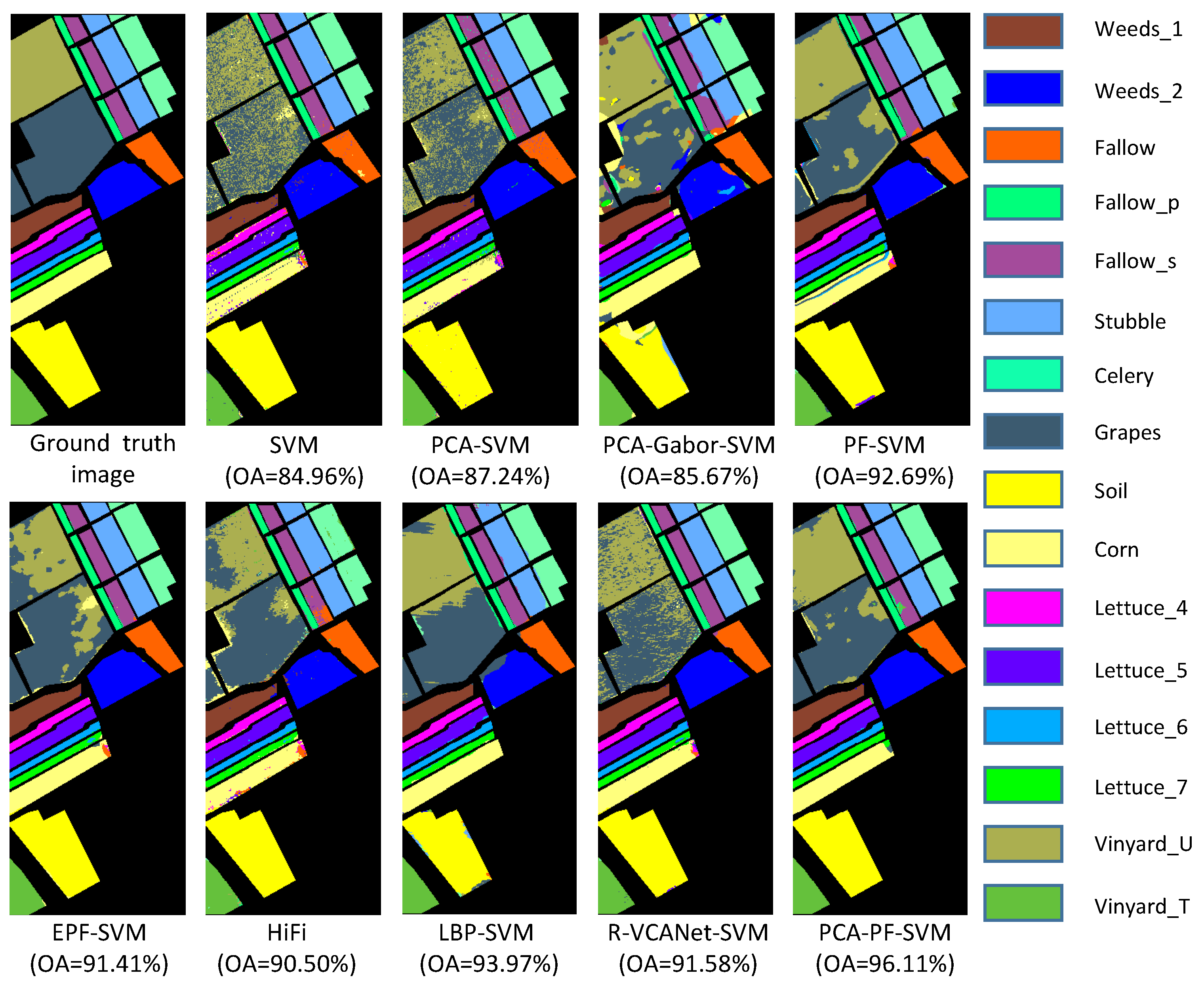
3.4. Experimental Results
4. Conclusions
Author Contributions
Funding
Acknowledgments
Conflicts of Interest
References
- Jia, X.; Kuo, B.C.; Crawford, M.M. Feature mining for hyperspectral image classification. Proc. IEEE 2013, 101, 676–697. [Google Scholar] [CrossRef]
- Fauvel, M.; Tarabalka, Y.; Benediktsson, J.A.; Chanussot, J.; Tilton, J.C. Advances in spectral-spatial classification of hyperspectral images. Proc. IEEE 2013, 101, 652–675. [Google Scholar] [CrossRef]
- Han, Y.; Li, J.; Zhang, Y. Sea Ice Detection Based on an Improved Similarity Measurement Method Using Hyperspectral Data. Sensors 2017, 17, 1124. [Google Scholar] [Green Version]
- Wong, E.; Minnett, P. Retrieval of the Ocean Skin Temperature Profiles From Measurements of Infrared Hyperspectral Radiometers—Part II: Field Data Analysis. IEEE Trans. Geosci. Remote Sens. 2016, 54, 1891–1904. [Google Scholar] [CrossRef]
- Zhang, T.; Wei, W.; Zhao, B. A Reliable Methodology for Determining Seed Viability by Using Hyperspectral Data from Two Sides of Wheat Seeds. Sensors 2018, 18, 813. [Google Scholar] [CrossRef] [PubMed]
- Behmann, J.; Acebron, K.; Emin, D. Specim IQ: Evaluation of a New, Miniaturized Handheld Hyperspectral Camera and Its Application for Plant Phenotyping and Disease Detection. Sensors 2018, 18, 441. [Google Scholar] [CrossRef] [PubMed]
- Sandino, J.; Pegg, G.; Gonzalez, F. Aerial Mapping of Forests Affected by Pathogens Using UAVs, Hyperspectral Sensors, and Artificial Intelligence. Sensors 2018, 18, 944. [Google Scholar] [CrossRef] [PubMed]
- Ma, N.; Peng, Y.; Wang, S. An Unsupervised Deep Hyperspectral Anomaly Detector. Sensors 2018, 18, 693. [Google Scholar] [CrossRef] [PubMed]
- Jiang, J.; Ma, J.; Wang, Z.; Chen, C. Hyperspectral Image Classification in the Presence of Noisy Labels. IEEE Trans. Geosci. Remote Sens. 2018, 1, 99. [Google Scholar]
- Ma, J.; Jiang, J.; Zhou, H.; Zhao, J.; Guo, X. Guided Locality Preserving Feature Matching for Remote Sensing Image Registration. IEEE Trans. Geosci. Remote Sens. 2018. [Google Scholar] [CrossRef]
- Pal, M.; Foody, G. Feature Selection for Classification of Hyperspectral Data by SVM. IEEE Trans. Geosci. Remote Sens. 2010, 48, 2297–2307. [Google Scholar] [CrossRef] [Green Version]
- Huo, H.; Guo, J.; Li, Z. Hyperspectral Image Classification for Land Cover Based on an Improved Interval Type-II Fuzzy C-Means Approach. Sensors 2018, 18, 363. [Google Scholar] [CrossRef] [PubMed]
- Tong, F.; Tong, H.; Jiang, J.; Zhang, Y. Multiscale union regions adaptive sparse representation for hyperspectral image classification. Remote Sens. 2017, 9, 872. [Google Scholar] [CrossRef]
- Ma, J.; Jiang, J.; Liu, C.; Li, Y. Feature guided Gaussian mixture model with semi-supervised EM and local geometric constraint for retinal image registration. Inf. Sci. 2017, 417, 128–142. [Google Scholar] [CrossRef]
- Ma, J.; Chen, C.; Li, C.; Huang, J. Infrared and visible image fusion via gradient transfer and total variation minimization. Inf. Fusion 2016, 31, 100–109. [Google Scholar] [CrossRef]
- Ma, J.; Ma, Y.; Li, C. Infrared and visible image fusion methods and applications: A survey. Inf. Fusion 2019, 45, 153–178. [Google Scholar] [CrossRef]
- Jon, D.; David, M. Supervised Topic Models. Adv. Neural Inf. Process. Syst. 2008, 20, 121–128. [Google Scholar]
- Jiang, X.; Fang, X.; Chen, Z. Supervised Gaussian Process Latent Variable Model for Hyperspectral Image Classification. IEEE Geosci. Remote Sens. Lett. 2017, 14, 1–5. [Google Scholar] [CrossRef]
- Lee, H.; Kim, M.; Jeong, D. Detection of cracks on tomatoes using a hyperspectral near-infrared reflectance imaging system. Sensors 2014, 14, 18837–18850. [Google Scholar] [CrossRef] [PubMed]
- Kuo, B.; Li, C.; Yang, J. Kernel Nonparametric Weighted Feature Extraction for Hyperspectral Image Classification. IEEE Trans. Geosci. Remote Sens. 2009, 47, 1139–1155. [Google Scholar]
- Jolliffe, I. Principal Component Analysis, 2nd ed.; Springer: New York, NY, USA, 2002; Volume 98. [Google Scholar]
- Boukhechba, K.; Wu, H.; Bazine, R. DCT-Based Preprocessing Approach for ICA in Hyperspectral Data Analysis. Sensors 2018, 18, 1138. [Google Scholar] [CrossRef] [PubMed]
- Jiang, J.; Ma, J.; Chen, C.; Wang, Z.; Cai, Z.; Wang, L. SuperPCA: A Superpixelwise Principal Component Analysis Approach for Unsupervised Feature Extraction of Hyperspectral Imagery. IEEE Trans. Geosci. Remote Sens. 2018. [Google Scholar] [CrossRef]
- Song, Y.; Nie, F.; Zhang, C. A unified framework for semi-supervised dimensionality reduction. Pattern Recognit. 2008, 41, 2789–2799. [Google Scholar] [CrossRef]
- Chen, C.; Li, W.; Tramel, E.W.; Cui, M.; Prasad, S.; Fowler, J.E. Spectral–spatial preprocessing using multihypothesis prediction for noise-robust hyperspectral image classification. IEEE J. Sel. Top. Appl. Earth Obs. Remote Sens. 2014, 7, 1047–1059. [Google Scholar] [CrossRef]
- Chen, C.; Li, W.; Su, H.; Liu, K. Spectral-spatial classification of hyperspectral image based on kernel extreme learning machine. Remote Sens. 2014, 6, 5795–5814. [Google Scholar] [CrossRef]
- Jiang, J.; Chen, C.; Yu, Y. Spatial-Aware Collaborative Representation for Hyperspectral Remote Sensing Image Classification. IEEE Geosci. Remote Sens. Lett. 2017, 14, 404–408. [Google Scholar] [CrossRef]
- Li, W.; Du, Q. Gabor-Filtering-Based Nearest Regularized Subspace for Hyperspectral Image Classification. IEEE J. Sel. Top. Appl. Earth Obs. Remote Sens. 2014, 7, 1012–1022. [Google Scholar] [CrossRef]
- Kang, X.; Li, S.; Benediktsson, J. Spectral–Spatial Hyperspectral Image Classification With Edge-Preserving Filtering. IEEE Trans. Geosci. Remote Sens. 2014, 52, 2666–2677. [Google Scholar] [CrossRef]
- Pan, B.; Zhen, W.; Xu, X.j. Hierarchical Guidance Filtering-Based Ensemble Classification for Hyperspectral Images. IEEE Trans. Geosci. Remote Sens. 2017, 55, 4177–4189. [Google Scholar] [CrossRef]
- Zhou, Y.; Wei, Y. Learning Hierarchical Spectral-Spatial Features for Hyperspectral Image Classification. IEEE Trans. Cybern. 2016, 46, 1667–1678. [Google Scholar] [CrossRef] [PubMed]
- Wei, Y.; Zhou, Y.; Li, H. Spectral-Spatial Response for Hyperspectral Image Classification. Remote Sens. 2017, 9, 203. [Google Scholar] [CrossRef]
- Yu, S.; Liang, X.; Molaei, M. Joint Multiview Fused ELM Learning with Propagation Filter for Hyperspectral Image Classification. In Proceedings of the Asian Conference on Computer Vision, Taipei, Taiwan, 20–24 November 2016; pp. 374–388. [Google Scholar]
- Chang, J.; Wang, Y. Propagated image filtering. In Proceedings of the IEEE Conference on Computer Vision and Pattern Recognit, Boston, MA, USA, 7–12 June 2015; Volume 1, pp. 10–18. [Google Scholar]
- Li, J.; Bioucas-Dias, J.; Plaza, A. Spectral–Spatial Classification of Hyperspectral Data Using Loopy Belief Propagation and Active Learning. IEEE Trans. Geosci. Remote Sens. 2013, 51, 844–856. [Google Scholar] [CrossRef]
- Prasad, S.; Bruce, L. Limitations of Principal Components Analysis for Hyperspectral Target Recognition. IEEE Geosci. Remote Sens. Lett. 2008, 5, 625–629. [Google Scholar] [CrossRef]
- Li, W.; Chen, C.; Su, H.; Du, Q. Local Binary Patterns and Extreme Learning Machine for Hyperspectral Imagery Classification. IEEE Trans. Geosci. Remote Sens. 2015, 53, 3681–3693. [Google Scholar] [CrossRef]
- Pan, B.; Shi, Z.; Xu, X. R-VCANet: A New Deep-Learning-Based Hyperspectral Image Classification Method. IEEE J. Sel. Top. Appl. Earth Obs. Remote Sens. 2017, 10, 1975–1986. [Google Scholar] [CrossRef]
- Chang, C.; Lin, C. LIBSVM: A library for support vector machines. ACM Trans. Intell. Syst. Technol. (TIST) 2011, 2, 27. [Google Scholar] [CrossRef]
- Chen, Y.; Lin, Z.; Zhao, X.; Wang, G.; Gu, Y. Deep Learning-Based Classification of Hyperspectral Data. IEEE J. Sel. Top. Appl. Earth Obs. Remote Sens. 2017, 7, 2094–2107. [Google Scholar] [CrossRef]
- Pan, B.; Shi, Z.; Zhang, N.; Xie, S. Hyperspectral Image Classification Based on Nonlinear Spectral–Spatial Network. IEEE Geosci. Remote Sens. Lett. 2016, 13, 1782–1786. [Google Scholar] [CrossRef]
- Chen, Y.; Zhao, X.; Jia, X. Spectral–Spatial Classification of Hyperspectral Data Based on Deep Belief Network. IEEE J. Sel. Top. Appl. Earth Obs. Remote Sens. 2015, 8, 2381–2392. [Google Scholar] [CrossRef]

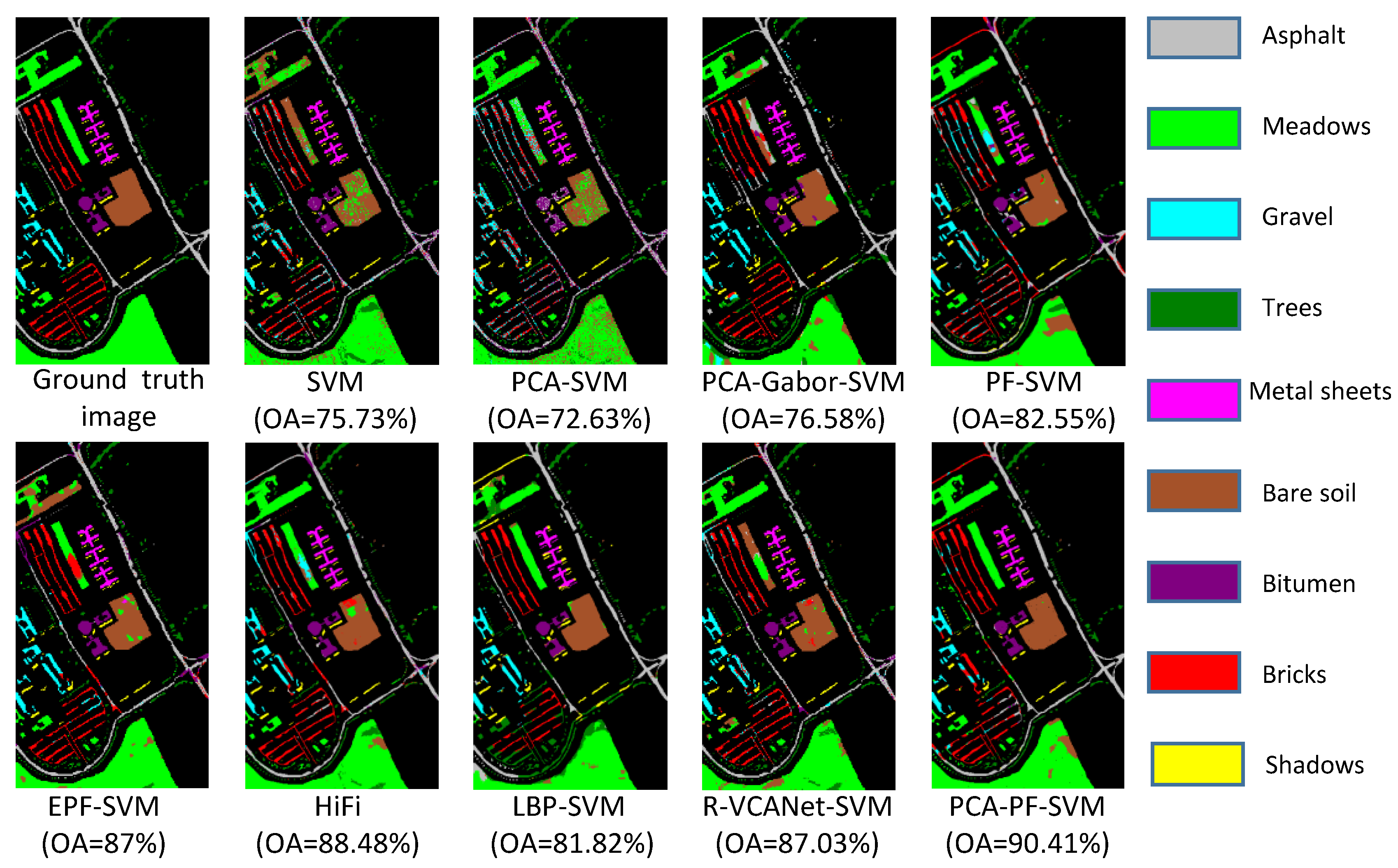
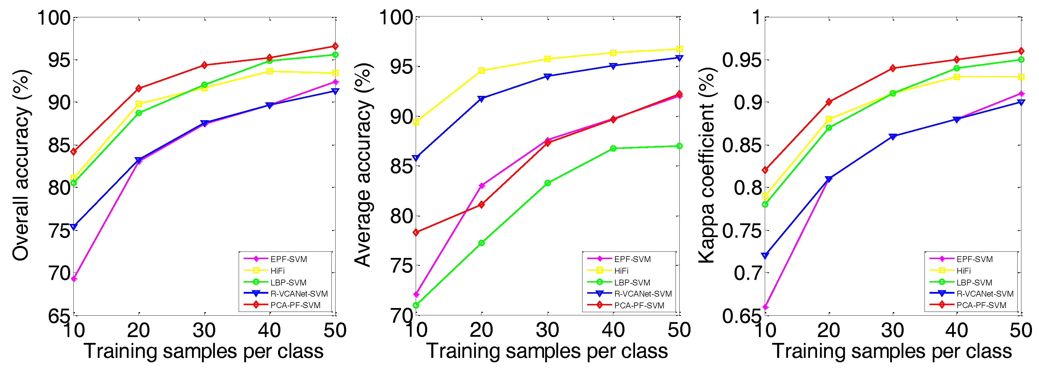
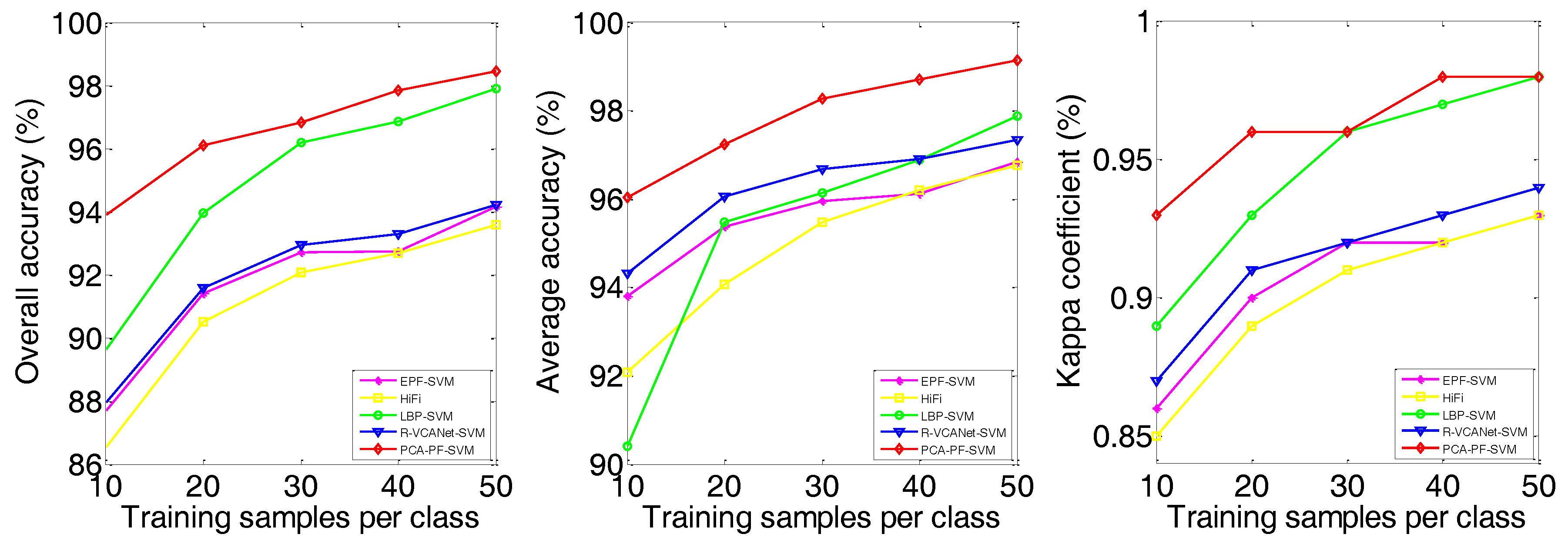
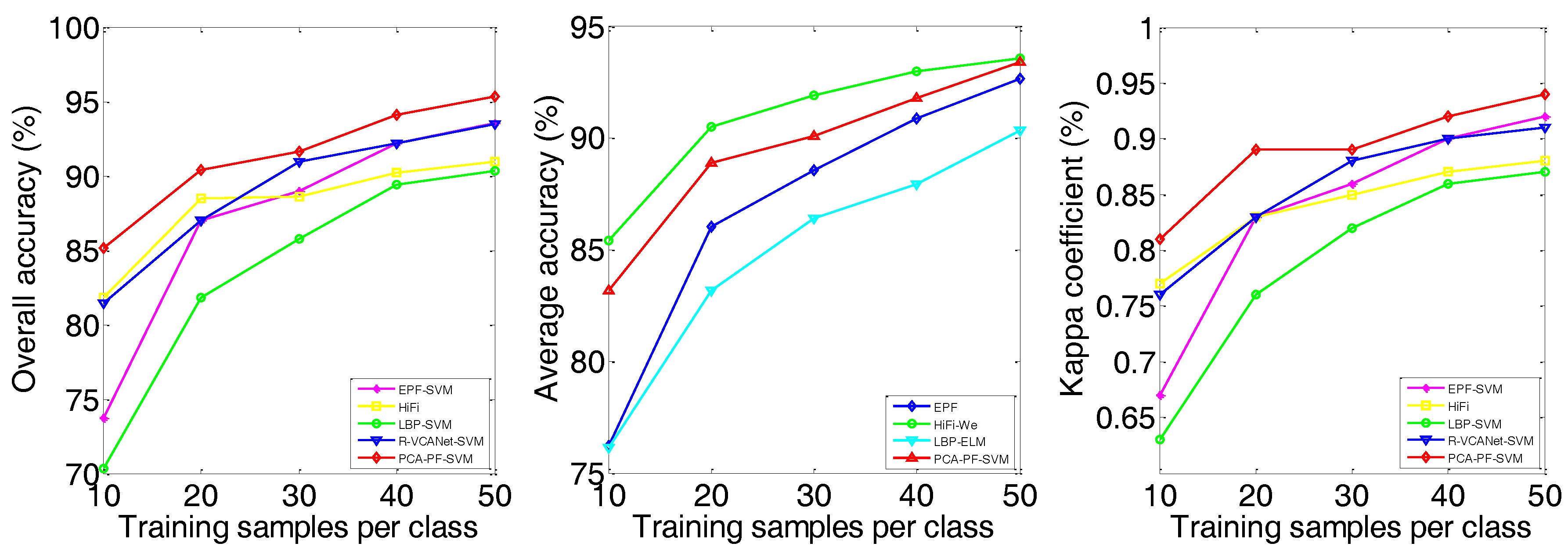
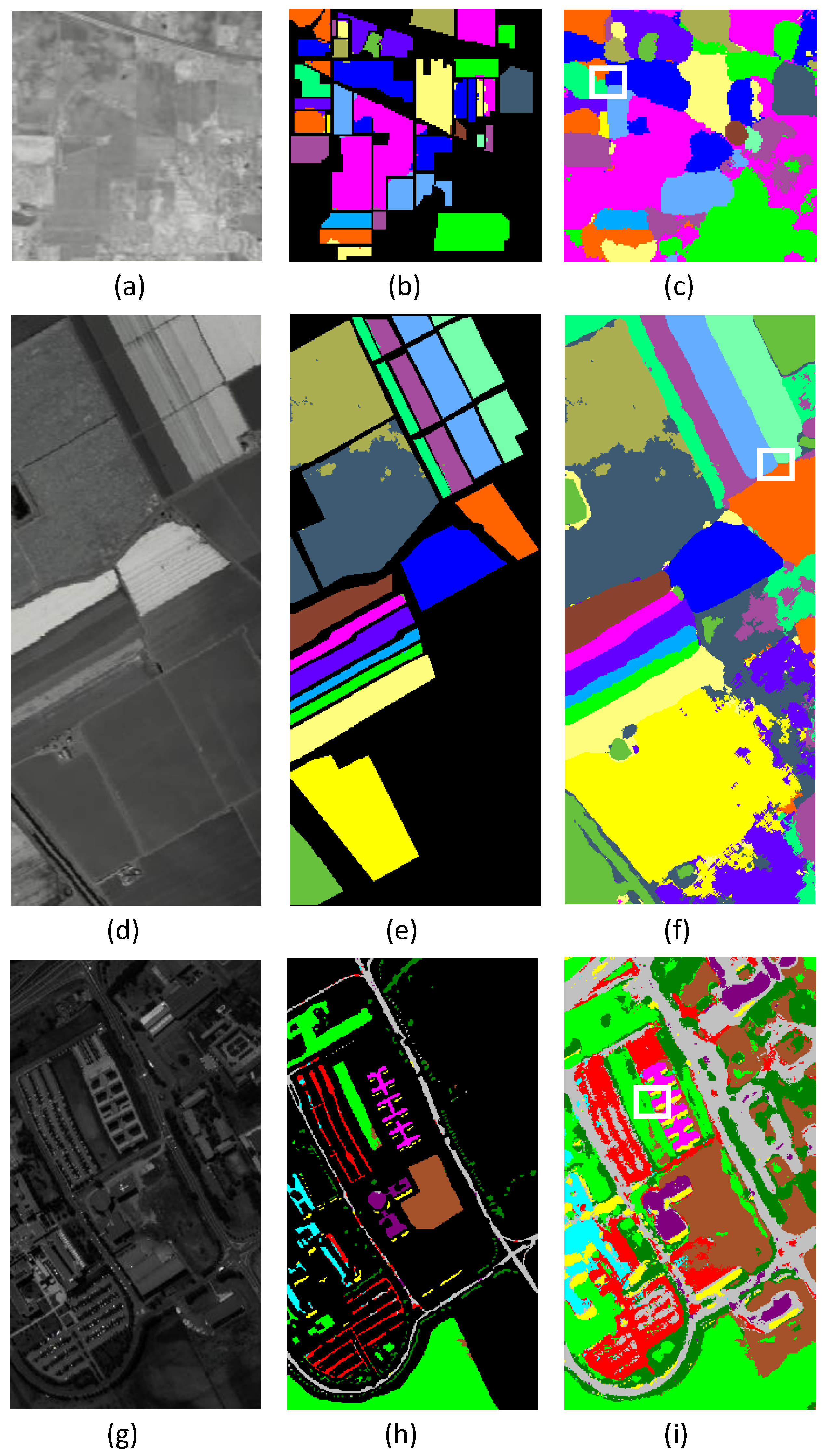

| Indian Pines | Salinas | University of Pavia | ||||||
|---|---|---|---|---|---|---|---|---|
| Class | Train | Test | Class | Train | Test | Class | Train | Test |
| Aifalfa | 20 | 26 | weeds_1 | 20 | 1989 | Asphalt | 20 | 18,629 |
| Corn_n | 20 | 1408 | weeds_2 | 20 | 3706 | Meadows | 20 | 2079 |
| Corn_m | 20 | 810 | fallow | 20 | 1956 | Gravel | 20 | 3044 |
| Corn | 20 | 217 | fallow_p | 20 | 1374 | Trees | 20 | 1325 |
| Grass_m | 20 | 463 | fallow_s | 20 | 2658 | Sheets | 20 | 5009 |
| Grass_t | 20 | 710 | stubble | 20 | 3939 | Soil | 20 | 1310 |
| Grass_p | 14 | 14 | Celery | 20 | 3559 | Bitumen | 20 | 3662 |
| Hay_w | 20 | 458 | Grapes | 20 | 11,251 | Bricks | 20 | 927 |
| Oats | 10 | 10 | Soil | 20 | 6183 | Shadows | 20 | 170 |
| Soybean_n | 20 | 952 | Corn | 20 | 3258 | |||
| Soybean_m | 20 | 2435 | Lettuce_4 | 20 | 1048 | |||
| Soybean_c | 20 | 573 | Lettuce_5 | 20 | 1907 | |||
| Wheat | 20 | 185 | Lettuce_6 | 20 | 896 | |||
| Woods | 20 | 1245 | Lettuce_7 | 20 | 1050 | |||
| Buildings | 20 | 366 | Vinyard_U | 20 | 7248 | |||
| Stone | 20 | 73 | Vinyard_T | 20 | 1787 | |||
| Class | SVM | PCA-SVM | PCA-Gabor-SVM | PF-SVM | EPF-SVM | HiFi | LBP-SVM | R-VCANet-SVM | PCA-PF-SVM |
|---|---|---|---|---|---|---|---|---|---|
| Aifalfa | 55.00 | 54.35 | 70.27 | 12.38 | 57.78 | 100.00 | 46.58 | 100.00 | 54.55 |
| Corn_n | 52.16 | 51.32 | 81.18 | 67.18 | 85.80 | 84.94 | 89.95 | 65.41 | 95.22 |
| Corn_m | 63.35 | 25.22 | 90.78 | 77.55 | 89.35 | 93.09 | 86.70 | 85.31 | 94.97 |
| Corn | 53.33 | 28.45 | 82.20 | 72.53 | 43.06 | 87.10 | 91.85 | 97.24 | 91.44 |
| Grass_m | 82.80 | 75.81 | 97.37 | 90.89 | 92.93 | 92.01 | 88.72 | 91.36 | 72.16 |
| Grass_t | 85.91 | 86.62 | 96.19 | 87.59 | 91.93 | 97.61 | 85.70 | 96.48 | 100.00 |
| Grass_p | 37.14 | 53.85 | 45.16 | 35.00 | 82.35 | 100.00 | 30.00 | 100.00 | 18.92 |
| Hay_w | 97.89 | 99.76 | 88.59 | 100.00 | 100.00 | 99.78 | 88.49 | 99.13 | 100.00 |
| Oats | 27.27 | 38.89 | 24.39 | 8.85 | 100.00 | 100.00 | 13.89 | 100.00 | 45.45 |
| Soybean_n | 57.38 | 29.14 | 95.84 | 68.79 | 66.32 | 93.70 | 74.14 | 83.61 | 84.34 |
| Soybean_m | 71.57 | 51.75 | 87.75 | 91.33 | 92.13 | 78.52 | 97.06 | 71.79 | 95.90 |
| Soybean_c | 37.88 | 36.69 | 93.13 | 68.58 | 52.77 | 94.24 | 85.89 | 87.43 | 88.51 |
| Wheat | 88.14 | 96.83 | 77.02 | 95.81 | 100.00 | 99.46 | 83.12 | 99.46 | 95.85 |
| Woods | 92.55 | 93.98 | 95.49 | 96.61 | 96.94 | 98.23 | 99.84 | 95.74 | 100.00 |
| Buildings | 39.31 | 53.67 | 90.20 | 74.44 | 88.99 | 93.99 | 95.87 | 95.36 | 72.58 |
| Stone | 95.77 | 87.65 | 76.04 | 34.45 | 87.95 | 100.00 | 78.43 | 100.00 | 87.01 |
| OA | 66.27 ± 2.46 | 55.45 ± 4.38 | 88.99 ± 1.33 | 78.33 ± 1.69 | 83.03 ± 1.85 | 89.82 ± 2.01 | 88.70 ± 1.93 | 83.23 ± 1.75 | 91.59 ± 1.32 |
| AA | 64.84 ± 2.28 | 60.25 ± 5.63 | 80.73 ± 1.60 | 67.62 ± 1.52 | 83.02 ± 3.19 | 94.54 ± 0.97 | 77.26 ± 2.58 | 91.77 ± 0.82 | 81.06 ± 3.91 |
| kappa | 0.62 ± 0.02 | 0.50 ± 0.04 | 0.87 ± 0.02 | 0.76 ± 0.02 | 0.81 ± 0.02 | 0.88 ± 0.02 | 0.87 ± 0.02 | 0.81 ± 0.01 | 0.90 ± 0.01 |
| Class | SVM | PCA-SVM | PCA-Gabor-SVM | PF-SVM | EPF-SVM | HiFi | LBP-SVM | R-VCANet-SVM | PCA-PF-SVM |
|---|---|---|---|---|---|---|---|---|---|
| weeds_1 | 98.05 | 100.00 | 88.18 | 98.07 | 100.00 | 98.49 | 99.40 | 99.90 | 100.00 |
| weeds_2 | 99.37 | 99.43 | 88.99 | 99.92 | 99.89 | 98.70 | 99.26 | 99.84 | 99.84 |
| fallow | 91.22 | 94.35 | 82.46 | 93.93 | 94.91 | 99.80 | 97.92 | 99.39 | 100.00 |
| fallow_p | 97.68 | 94.41 | 73.87 | 86.13 | 97.86 | 97.45 | 83.89 | 99.56 | 91.79 |
| fallow_s | 97.00 | 95.24 | 81.13 | 97.62 | 99.96 | 88.75 | 97.28 | 99.62 | 99.52 |
| stubble | 100.00 | 99.95 | 92.22 | 99.95 | 99.92 | 99.59 | 95.13 | 99.97 | 99.97 |
| Celery | 99.94 | 100.00 | 96.04 | 98.22 | 100.00 | 96.60 | 94.66 | 98.17 | 100.00 |
| Grapes | 72.98 | 76.85 | 92.01 | 91.63 | 82.04 | 82.13 | 91.57 | 78.54 | 95.28 |
| Soil | 98.59 | 99.00 | 97.29 | 99.49 | 99.48 | 99.97 | 99.97 | 99.26 | 99.97 |
| Corn | 79.39 | 93.32 | 64.75 | 92.48 | 85.06 | 87.97 | 99.04 | 94.69 | 97.76 |
| Lettuce_4 | 93.65 | 91.02 | 95.66 | 95.42 | 98.21 | 96.18 | 98.96 | 98.76 | 100.00 |
| Lettuce_5 | 94.34 | 91.97 | 97.63 | 96.07 | 100.00 | 99.48 | 99.89 | 100.00 | 100.00 |
| Lettuce_6 | 93.37 | 91.14 | 84.29 | 76.19 | 96.10 | 97.21 | 92.64 | 94.31 | 98.33 |
| Lettuce_7 | 92.29 | 94.26 | 90.26 | 99.41 | 99.20 | 92.67 | 95.97 | 96.86 | 93.09 |
| Vinyard_U | 54.30 | 58.25 | 73.37 | 77.59 | 73.97 | 73.17 | 83.00 | 85.32 | 85.01 |
| Vinyard_T | 94.44 | 99.54 | 94.03 | 98.59 | 99.49 | 96.75 | 99.17 | 99.27 | 95.21 |
| OA | 84.96 ± 1.17 | 87.24 ± 1.73 | 85.67 ± 1.99 | 92.69 ± 1.38 | 91.41 ± 2.29 | 90.50 ± 1.32 | 93.97 ± 2.28 | 91.58 ± 1.09 | 96.11 ± 0.86 |
| AA | 91.04 ± 0.53 | 92.42 ± 0.93 | 87.01 ± 1.78 | 93.80 ± 0.85 | 95.38 ± 0.85 | 94.06 ± 0.68 | 95.48 ± 1.62 | 96.05 ± 0.40 | 97.24 ± 0.45 |
| kappa | 0.83 ± 0.01 | 0.86 ± 0.02 | 0.84 ± 0.02 | 0.92 ± 0.02 | 0.90 ± 0.03 | 0.89 ± 0.01 | 0.93 ± 0.03 | 0.91 ± 0.01 | 0.96 ± 0.01 |
| Class | SVM | PCA-SVM | PCA-Gabor-SVM | PF-SVM | EPF-SVM | HiFi | LBP-SVM | R-VCANet-SVM | PCA-PF-SVM |
|---|---|---|---|---|---|---|---|---|---|
| Asphalt | 87.52 | 82.14 | 72.39 | 85.47 | 98.05 | 80.40 | 84.36 | 79.96 | 92.30 |
| Meadows | 91.00 | 90.51 | 95.96 | 97.60 | 97.40 | 89.74 | 97.98 | 83.39 | 99.47 |
| Gravel | 61.72 | 39.42 | 75.01 | 56.17 | 89.16 | 82.92 | 72.93 | 88.12 | 84.96 |
| Trees | 70.10 | 79.54 | 40.27 | 80.30 | 96.20 | 83.64 | 51.19 | 96.75 | 76.68 |
| Sheets | 98.42 | 100.00 | 88.21 | 99.25 | 95.05 | 99.17 | 86.32 | 100.00 | 99.92 |
| Soil | 46.04 | 53.61 | 68.69 | 70.30 | 64.27 | 89.72 | 75.02 | 93.57 | 84.80 |
| Bitumen | 54.64 | 32.06 | 78.94 | 71.72 | 58.20 | 96.79 | 76.85 | 99.01 | 85.61 |
| Bricks | 80.23 | 57.68 | 80.20 | 60.79 | 76.20 | 92.55 | 78.43 | 88.39 | 79.43 |
| Shadows | 100.00 | 99.35 | 49.44 | 83.23 | 99.89 | 99.46 | 45.34 | 100.00 | 96.95 |
| OA | 75.73 ± 1.64 | 72.63 ± 3.40 | 76.58 ± 2.98 | 82.55 ± 3.41 | 87.00 ± 2.43 | 88.48 ± 1.90 | 81.82 ± 1.68 | 87.03 ± 1.19 | 90.41 ± 1.90 |
| AA | 76.63 ± 1.43 | 70.48 ± 2.41 | 72.12 ± 2.81 | 78.31 ± 3.34 | 86.05 ± 2.39 | 90.49 ± 0.97 | 74.27 ± 2.19 | 91.17 ± 0.89 | 88.90 ± 2.05 |
| kappa | 0.69 ± 0.02 | 0.65 ± 0.04 | 0.70 ± 0.03 | 0.78 ± 0.04 | 0.83 ± 0.03 | 0.83 ± 0.02 | 0.76 ± 0.02 | 0.83 ± 0.01 | 0.89 ± 0.02 |
| Method | Quality Indexes | Indian Pines | Salinas | University of Pavia | ||||||||||||
|---|---|---|---|---|---|---|---|---|---|---|---|---|---|---|---|---|
| Training Samples Perclass | Training Samples Perclass | Training Samples Perclass | ||||||||||||||
| 10 | 20 | 30 | 40 | 50 | 10 | 20 | 30 | 40 | 50 | 10 | 20 | 30 | 40 | 50 | ||
| SVM | OA | 57.43 | 66.27 | 73.31 | 75.94 | 78.66 | 82.64 | 84.96 | 86.42 | 86.20 | 87.70 | 67.02 | 75.73 | 78.95 | 82.30 | 83.78 |
| AA | 55.87 | 64.84 | 69.84 | 72.67 | 75.86 | 88.87 | 91.04 | 91.38 | 91.77 | 92.75 | 69.12 | 76.63 | 77.69 | 80.23 | 81.36 | |
| kappa | 0.52 | 0.62 | 0.70 | 0.73 | 0.76 | 0.81 | 0.83 | 0.85 | 0.85 | 0.86 | 0.59 | 0.69 | 0.73 | 0.77 | 0.79 | |
| PCA-SVM | OA | 47.89 | 55.45 | 58.47 | 62.07 | 66.67 | 84.47 | 87.24 | 88.59 | 88.37 | 89.30 | 61.71 | 72.63 | 76.53 | 77.90 | 80.41 |
| AA | 53.23 | 60.25 | 64.14 | 67.02 | 72.15 | 88.98 | 92.42 | 93.89 | 93.99 | 94.40 | 60.60 | 70.48 | 74.04 | 75.29 | 77.15 | |
| kappa | 0.42 | 0.50 | 0.53 | 0.57 | 0.62 | 0.83 | 0.88 | 0.87 | 0.87 | 0.88 | 0.52 | 0.65 | 0.70 | 0.72 | 0.75 | |
| PCA-Gabor-SVM | OA | 76.03 | 88.99 | 93.06 | 94.64 | 96.09 | 73.62 | 85.67 | 89.29 | 93.08 | 94.46 | 65.51 | 76.58 | 81.26 | 84.30 | 86.18 |
| AA | 75.90 | 80.73 | 86.93 | 88.79 | 91.78 | 76.95 | 87.01 | 90.49 | 93.70 | 94.91 | 63.76 | 72.12 | 77.19 | 80.11 | 83.28 | |
| kappa | 0.73 | 0.87 | 0.92 | 0.94 | 0.96 | 0.71 | 0.84 | 0.88 | 0.92 | 0.94 | 0.57 | 0.70 | 0.76 | 0.80 | 0.82 | |
| PF-SVM | OA | 64.77 | 78.33 | 84.19 | 87.84 | 90.40 | 88.69 | 92.69 | 94.28 | 95.16 | 95.46 | 71.23 | 82.55 | 87.62 | 89.13 | 91.73 |
| AA | 59.06 | 67.62 | 73.27 | 77.47 | 82.39 | 91.24 | 93.80 | 95.77 | 96.42 | 96.64 | 68.91 | 78.31 | 82.82 | 83.76 | 87.38 | |
| kappa | 0.61 | 0.76 | 0.82 | 0.86 | 0.89 | 0.97 | 0.92 | 0.94 | 0.95 | 0.95 | 0.64 | 0.78 | 0.84 | 0.86 | 0.89 | |
| EPF-SVM | OA | 69.32 | 83.03 | 87.41 | 89.63 | 92.41 | 87.71 | 91.41 | 92.70 | 92.73 | 94.15 | 73.76 | 87.00 | 88.97 | 92.19 | 93.57 |
| AA | 72.06 | 83.02 | 87.60 | 89.74 | 92.02 | 93.80 | 95.38 | 95.96 | 96.12 | 96.85 | 76.21 | 86.05 | 88.56 | 90.89 | 92.66 | |
| kappa | 0.66 | 0.81 | 0.86 | 0.88 | 0.91 | 0.86 | 0.90 | 0.92 | 0.92 | 0.93 | 0.67 | 0.83 | 0.86 | 0.90 | 0.92 | |
| HiFi | OA | 81.08 | 89.82 | 91.65 | 93.63 | 93.44 | 86.53 | 90.50 | 92.08 | 92.67 | 93.59 | 81.83 | 88.48 | 88.64 | 90.22 | 90.94 |
| AA | 89.44 | 94.54 | 95.74 | 96.36 | 96.72 | 92.08 | 94.06 | 95.47 | 96.20 | 96.76 | 85.40 | 90.49 | 91.91 | 92.99 | 93.58 | |
| kappa | 0.79 | 0.88 | 0.91 | 0.93 | 0.93 | 0.85 | 0.89 | 0.91 | 0.92 | 0.93 | 0.77 | 0.83 | 0.85 | 0.87 | 0.88 | |
| LBP-SVM | OA | 80.49 | 88.70 | 92.01 | 94.85 | 95.58 | 89.65 | 93.97 | 96.18 | 96.86 | 97.91 | 70.35 | 81.82 | 85.75 | 89.39 | 90.34 |
| AA | 70.96 | 77.26 | 83.29 | 86.72 | 87.00 | 90.41 | 95.48 | 96.13 | 96.88 | 97.87 | 66.39 | 74.27 | 81.33 | 84.85 | 86.41 | |
| kappa | 0.78 | 0.87 | 0.91 | 0.94 | 0.95 | 0.89 | 0.93 | 0.96 | 0.97 | 0.98 | 0.63 | 0.76 | 0.82 | 0.86 | 0.87 | |
| R-VCANet-SVM | OA | 75.40 | 83.23 | 87.56 | 89.66 | 91.33 | 87.96 | 91.58 | 92.93 | 93.29 | 94.21 | 81.47 | 87.03 | 90.95 | 92.18 | 93.46 |
| AA | 85.82 | 91.77 | 94.00 | 95.05 | 95.88 | 94.32 | 96.05 | 96.68 | 96.91 | 97.34 | 87.21 | 92.13 | 93.51 | 94.48 | 95.51 | |
| kappa | 0.72 | 0.81 | 0.86 | 0.88 | 0.90 | 0.87 | 0.91 | 0.92 | 0.93 | 0.94 | 0.76 | 0.83 | 0.88 | 0.90 | 0.91 | |
| PCA-PF-SVM | OA | 84.20 | 91.59 | 94.32 | 95.23 | 96.55 | 93.91 | 96.11 | 96.83 | 97.84 | 98.45 | 85.14 | 90.41 | 91.62 | 94.12 | 95.34 |
| AA | 78.28 | 81.06 | 87.29 | 89.65 | 92.22 | 96.04 | 97.24 | 98.28 | 98.70 | 99.14 | 83.17 | 88.90 | 88.26 | 91.80 | 93.41 | |
| kappa | 0.82 | 0.90 | 0.94 | 0.95 | 0.96 | 0.93 | 0.96 | 0.96 | 0.98 | 0.98 | 0.81 | 0.89 | 0.89 | 0.92 | 0.94 | |
| Indian Pines | ||||||||||||
| Training Samples Perclass | PCA-Gabor-NRS | PCA-PF-NRS | LBP-ELM | PCA-PF-ELM | ||||||||
| OA | AA | kappa | OA | AA | kappa | OA | AA | kappa | OA | AA | kappa | |
| 10 | 68.46 | 61.32 | 0.65 | 84.50 | 76.99 | 0.83 | 80.89 | 89.16 | 0.79 | 83.15 | 90.43 | 0.81 |
| 20 | 82.56 | 75.63 | 0.80 | 90.82 | 83.84 | 0.90 | 88.37 | 93.62 | 0.87 | 91.44 | 95.32 | 0.90 |
| 30 | 88.93 | 83.28 | 0.87 | 93.73 | 87.69 | 0.93 | 92.57 | 96.09 | 0.92 | 94.35 | 96.81 | 0.94 |
| 40 | 91.99 | 87.17 | 0.91 | 94.79 | 89.67 | 0.94 | 94.42 | 96.76 | 0.94 | 95.69 | 97.68 | 0.95 |
| 50 | 93.71 | 89.21 | 0.93 | 95.72 | 90.08 | 0.95 | 95.76 | 97.77 | 0.95 | 97.08 | 98.37 | 0.97 |
| Salinas | ||||||||||||
| Training Samples Perclass | PCA-Gabor-NRS | PCA-PF-NRS | LBP-ELM | PCA-PF-ELM | ||||||||
| OA | AA | kappa | OA | AA | kappa | OA | AA | kappa | OA | AA | kappa | |
| 10 | 57.53 | 55.95 | 0.54 | 93.54 | 95.64 | 0.93 | 90.41 | 92.92 | 0.89 | 93.22 | 96.70 | 0.92 |
| 20 | 75.74 | 75.55 | 0.73 | 95.97 | 97.46 | 0.96 | 94.90 | 96.47 | 0.94 | 95.96 | 98.12 | 0.96 |
| 30 | 87.62 | 88.11 | 0.86 | 96.91 | 98.24 | 0.97 | 96.46 | 97.84 | 0.96 | 96.58 | 98.49 | 0.96 |
| 40 | 91.94 | 92.2 | 0.91 | 97.41 | 98.48 | 0.97 | 97.69 | 98.38 | 0.97 | 97.90 | 98.99 | 0.98 |
| 50 | 94.85 | 94.8 | 0.94 | 7.93 | 98.74 | 0.98 | 98.02 | 98.67 | 97.79 | 98.40 | 99.23 | 0.98 |
| University of Pavia | ||||||||||||
| Training Samples Perclass | PCA-Gabor-NRS | PCA-PF-NRS | LBP-ELM | PCA-PF-ELM | ||||||||
| OA | AA | kappa | OA | AA | kappa | OA | AA | kappa | OA | AA | kappa | |
| 10 | 50.86 | 51.76 | 0.41 | 80.73 | 78.73 | 0.75 | 73.98 | 76.15 | 0.67 | 82.18 | 82.47 | 0.77 |
| 20 | 63.07 | 62.57 | 0.55 | 89.18 | 86.87 | 0.86 | 82.47 | 82.9 | 0.78 | 89.42 | 89.09 | 0.86 |
| 30 | 69.39 | 67.65 | 0.62 | 93.06 | 91.04 | 0.91 | 86.52 | 86.42 | 0.82 | 91.13 | 91.26 | 0.88 |
| 40 | 76.64 | 75.21 | 0.71 | 94.48 | 92.77 | 0.93 | 88.83 | 87.93 | 0.85 | 92.69 | 92.52 | 0.90 |
| 50 | 82.26 | 81.09 | 0.78 | 95.21 | 93.73 | 0.94 | 90.77 | 90.36 | 0.88 | 94.60 | 93.42 | 0.93 |
© 2018 by the authors. Licensee MDPI, Basel, Switzerland. This article is an open access article distributed under the terms and conditions of the Creative Commons Attribution (CC BY) license (http://creativecommons.org/licenses/by/4.0/).
Share and Cite
Chen, Z.; Jiang, J.; Jiang, X.; Fang, X.; Cai, Z. Spectral-Spatial Feature Extraction of Hyperspectral Images Based on Propagation Filter. Sensors 2018, 18, 1978. https://doi.org/10.3390/s18061978
Chen Z, Jiang J, Jiang X, Fang X, Cai Z. Spectral-Spatial Feature Extraction of Hyperspectral Images Based on Propagation Filter. Sensors. 2018; 18(6):1978. https://doi.org/10.3390/s18061978
Chicago/Turabian StyleChen, Zhikun, Junjun Jiang, Xinwei Jiang, Xiaoping Fang, and Zhihua Cai. 2018. "Spectral-Spatial Feature Extraction of Hyperspectral Images Based on Propagation Filter" Sensors 18, no. 6: 1978. https://doi.org/10.3390/s18061978
APA StyleChen, Z., Jiang, J., Jiang, X., Fang, X., & Cai, Z. (2018). Spectral-Spatial Feature Extraction of Hyperspectral Images Based on Propagation Filter. Sensors, 18(6), 1978. https://doi.org/10.3390/s18061978


