Optimal Design of Electromagnetically Actuated MEMS Cantilevers


 , ,
, ,  and
and
Abstract
:1. Introduction
2. Materials and Methods
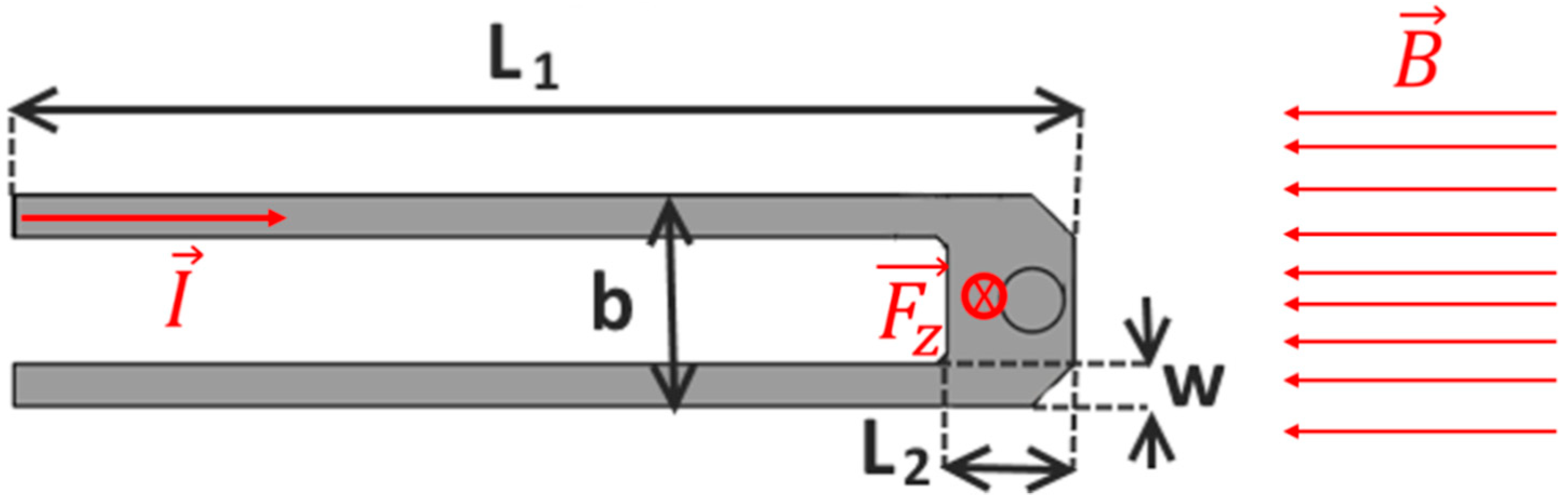
2.1. Optimal Design of an Electromagnetically Actuated Cantilever: Direct Problem
- the stiffness k of the cantilever;
- the resonance frequency f of the cantilever;
- the force Fz acting on the end region and its displacement Δz;
- the electric resistance R (power-loss related) of the Lorentz loop.
2.2. Optimal Design of an Electromagnetically Actuated Cantilever: Inverse Problem
- the stiffness k(g) of the cantilever is minimized;
- the resonance frequency f(g) is maximized;
- the displacement Δz(g) of the end region is maximized;
- the electric resistance R(g) of the Lorentz loop is minimized.
- w, arm width.
- L1, cantilever length.
- L2, tip length.
- b, cantilever width.
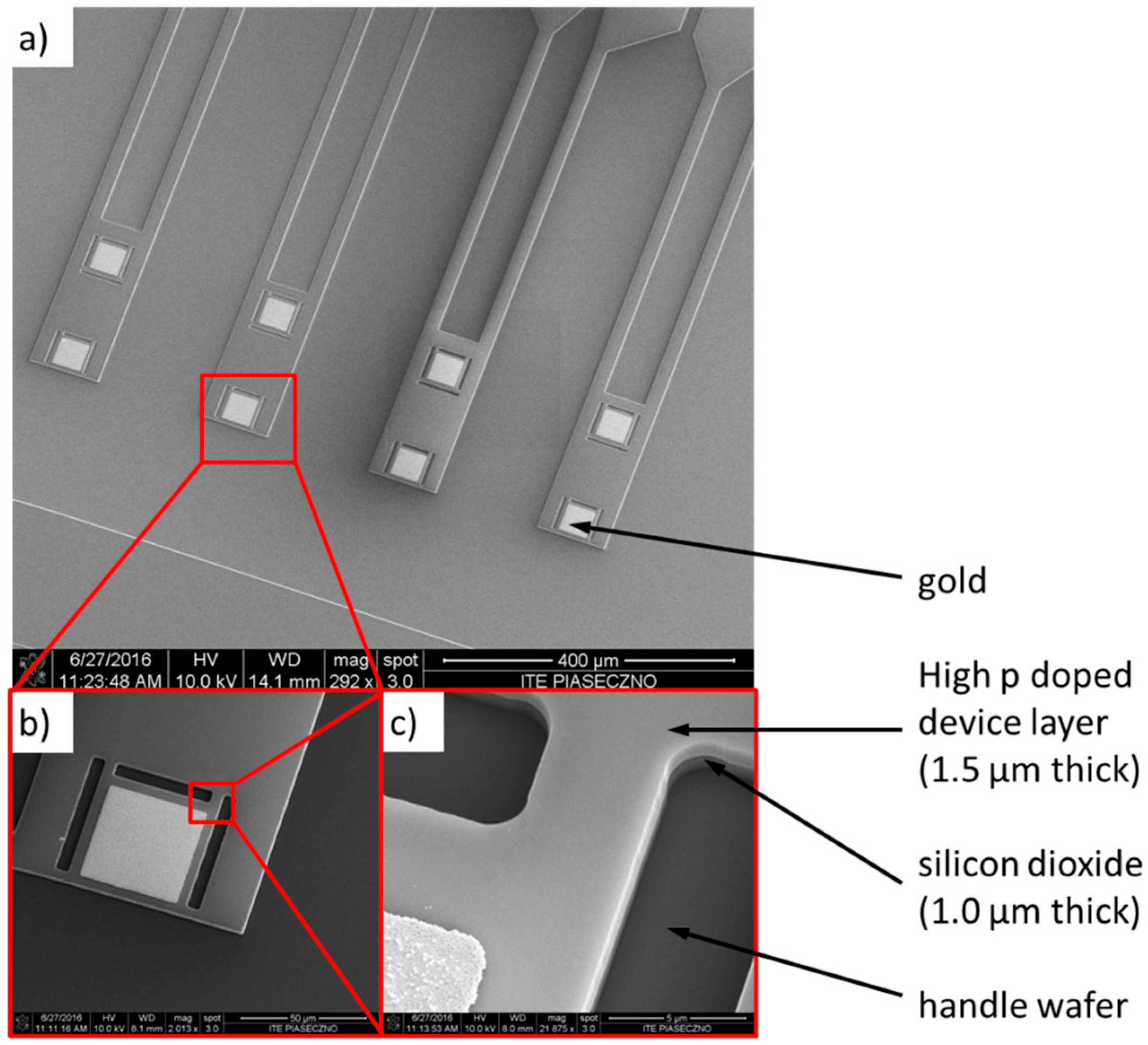
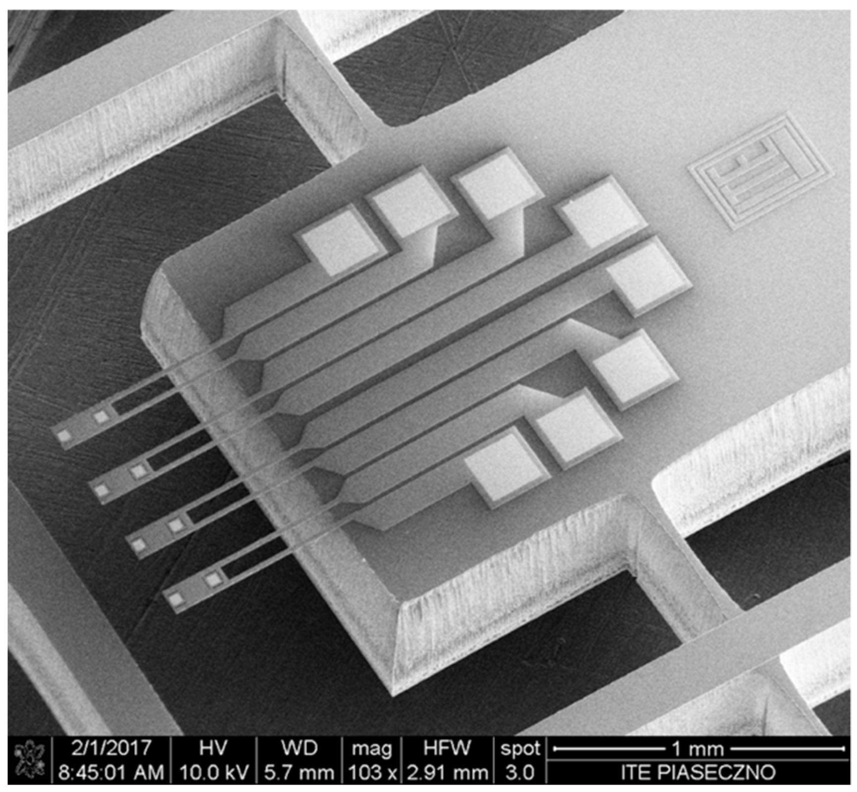
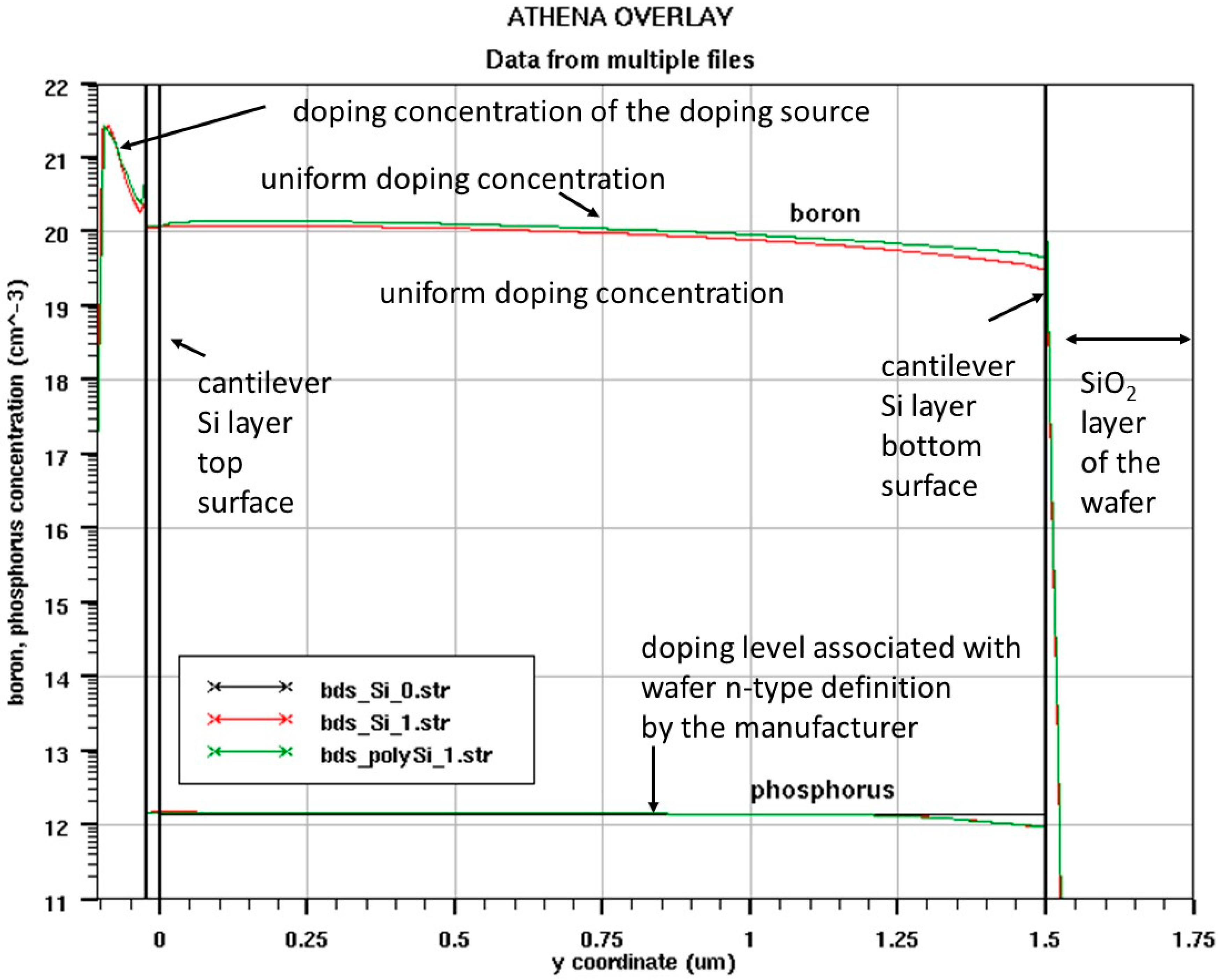
2.3. Fabrication Process
3. Results
3.1. Single-Objective Optimization Results
3.2. Bi-Objective Optimization Results
3.3. Tri-Objective Optimization Results
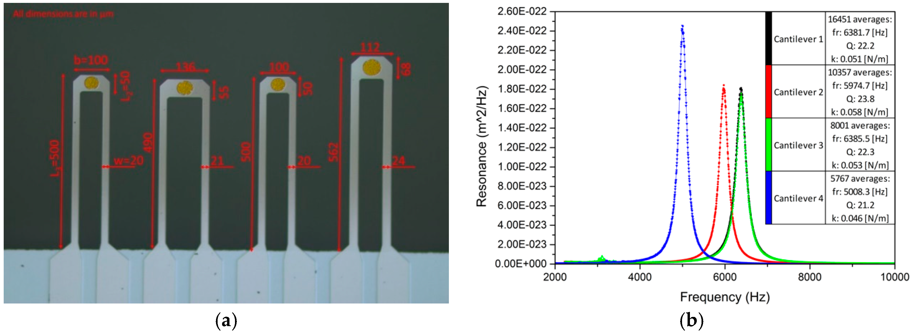
3.4. Measurements on Optimal Cantilevers
- -
- two cantilevers corresponding to initial design,
- -
- final design, according to Opt2fz optimization result
- -
- final design, according to Opt3 optimization result
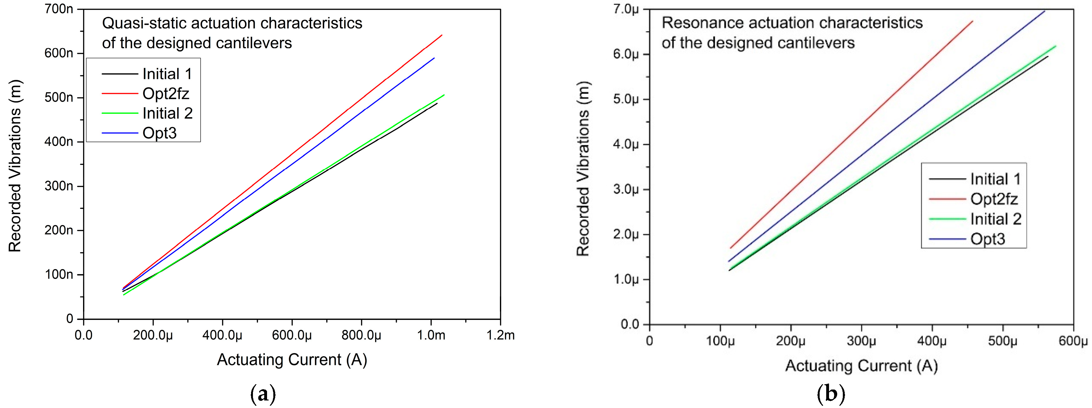
3.5. Electromagnetic Actuation of the Cantilevers
4. Discussion
5. Conclusions
Author Contributions
Funding
Conflicts of Interest
References
- Lang, H.P.; Hegner, M.; Gerber, C. Nanomechanical cantilever array sensors. In Springer Handbook of Nanotechnology; Springer: Berlin/Heidelberg, Germany, 2013; pp. 457–485. [Google Scholar]
- Gaspar, J.; Chu, V.; Conde, J.P. Electrostatic actuation of thin-film microelectromechanical structures. J. Appl. Phys. 2003, 93, 10018–10029. [Google Scholar] [CrossRef]
- Minne, S.C.; Manalis, S.R.; Quate, C.F. Parallel atomic force microscopy using cantilevers with integrated piezoresistive sensors and integrated piezoelectric actuators. Appl. Phys. Lett. 1995, 67. [Google Scholar] [CrossRef]
- Angelov, T.; Roeser, D.; Ivanov, T.; Gutschmidt, S.; Sattel, T.; Rangelow, I.W. Thermo-mechanical transduction suitable for high-speed scanning probe imaging and lithography. Microelectron. Eng. 2016, 154, 1–7. [Google Scholar] [CrossRef]
- Woszczyna, M.; Zawierucha, P.; Pałetko, P.; Zielony, M.; Gotszalk, T.; Sarov, Y.; Ivanov, T.; Frank, A.; Zöllner, J.-P.; Rangelow, I.W. Micromachined scanning proximal probes with integrated piezoresistive readout and bimetal actuator for high eigenmode operation. J. Vac. Sci. Technol. B 2010, 28. [Google Scholar] [CrossRef]
- Majstrzyk, W.; Ahmad, A.; Ivanov, T.; Reum, A.; Angelow, T.; Holz, M.; Gotszalk, T.; Rangelow, I.W. Thermomechanically and electromagnetically actuated piezoresistive cantilevers for fast-scanning probe microscopy investigations. Sens. Actuators A Phys. 2018, 276, 237–245. [Google Scholar] [CrossRef]
- Nieradka, K.M.; Kopiec, D.; Małozięć, G.; Kowalska, Z.; Grabiec, P.; Janus, P.; Sierakowski, A.; Domański, K.; Gotszalk, T. Fabrication and characterization of electromagnetically actuated microcantilevers for biochemical sensing, parallel AFM and nanomanipulation. Microelectron. Eng. 2012, 98, 676–679. [Google Scholar] [CrossRef]
- Shen, B.; Allegretto, W.; Hu, M.; Robinson, A. Cmos micromachined cantilever-in-cantilever devices with magnetic actuation. IEEE Electron Device Lett. 1996, 17, 372–374. [Google Scholar] [CrossRef]
- Adhikari, R.; Kaundal, R.; Sarkar, A.; Rana, P.; Das, A.K. The cantilever beam magnetometer: A simple teaching tool for magnetic characterization. Am. J. Phys. 2012, 80, 225. [Google Scholar] [CrossRef]
- Hsieh, C.H.; Dai, C.L.; Yang, M.Z. Fabrication and characterization of cmos-mems magnetic microsensors. Sensors 2013, 13, 14728–14738. [Google Scholar] [CrossRef] [PubMed]
- Rhoads, J.F.; Kumar, V.; Shaw, S.W.; Turner, K.L. The non-linear dynamics of electromagnetically actuated microbeam resonators with purely parametric excitations. Int. J. Non-Linear Mech. 2013, 55, 79–89. [Google Scholar] [CrossRef]
- Somnath, S.; Liu, J.O.; Bakir, M.; Prater, C.B.; King, W.P. Multifunctional atomic force microscope cantilevers with Lorentz force actuation and self-heating capability. Nanotechnology 2014, 25. [Google Scholar] [CrossRef] [PubMed]
- Majstrzyk, W.; Mognaschi, M.E.; Orłowska, K.; Di Barba, P.; Sierakowski, A.; Dobrowolski, R.; Grabiec, P.; Gotszalk, T. Electromagnetic cantilever reference for the calibration of optical nanodisplacement systems. Sens. Actuators A Phys. 2018. under revision. [Google Scholar]
- Fritz, J.; Baller, M.K.; Lang, H.P.; Strunz, T.; Meyer, E.; Güntherodt, H.J.; Delamarche, E.; Gerber, C.; Gimzewski, J.K. Stress at the solid-liquid interface of self-assembled monolayers on gold investigated with a nanomechanical sensor. Langmuir 2000, 16. [Google Scholar] [CrossRef]
- Kopiec, D.; Pałetko, P.; Nieradka, K.; Majstrzyk, W.; Kunicki, P.; Sierakowski, A.; Jóźwiak, G.; Gotszalk, T. Closed-loop surface stress compensation with an electromagnetically actuated microcantilever. Sens. Actuators B Chem. 2015, 228, 62–68. [Google Scholar] [CrossRef]
- Di Barba, P.; Mognaschi, M.E.; Venini, P.; Wiak, S. Biogeography-inspired multiobjective optimization for helping MEMS synthesis. Arch. Electr. Eng. 2017, 66, 607–623. [Google Scholar] [CrossRef] [Green Version]
- Tortonese, M.; Barrett, R.C.; Quate, C.F. Atomic resolution with an atomic force microscope using piezoresistive detection. Appl. Phys. Lett. 1993, 62. [Google Scholar] [CrossRef]
- Walters, D.A.; Cleveland, J.P.; Thomson, N.H.; Hansma, P.K.; Wendman, M.A.; Gurley, G.; Elings, V. Short cantilevers for atomic force microscopy. Rev. Sci. Instrum. 1996, 67. [Google Scholar] [CrossRef]
- Di Barba, P. Multiobjective Shape Design in Electricity and Magnetism; Springer-Verlag: Berlin, Germany, 2010. [Google Scholar]
- Di Barba, P.; Savini, A.; Wiak, S. Field Models in Electricity and Magnetism; Springer: Berlin, Germany, 2008. [Google Scholar]
- Di Barba, P.; Mognaschi, M.E.; Lowther, D.A.; Sykulski, J.K. A benchmark TEAM problem for multi-objective pareto optimization of electromagnetic devices. IEEE Trans. Magn. 2018, 54. [Google Scholar] [CrossRef]
- Di Barba, P.; Mognaschi, M.E. Industrial design with multiple criteria: Shape optimization of a permanent-magnet generator. IEEE Trans. Magn. 2009, 45, 1482–1485. [Google Scholar] [CrossRef]
- Costamagna, E.; Di Barba, P.; Mognaschi, M.E.; Savini, A. Fast algorithms for the design of complex-shape devices in electromechanics. In Studies in Computational Intelligence; Springer: Berlin, Germany, 2010; Volume 327, pp. 59–86. [Google Scholar]
- Gotszalk, T.; Grabiec, P.; Rangelow, I.W. Piezoresistive sensors for scanning probe microscopy. Ultramicroscopy 2000, 82, 39–48. [Google Scholar] [CrossRef]
- Buguin, A.; Du Roure, O.; Silberzan, P. Active atomic force microscopy cantilevers for imaging in liquids. Appl. Phys. Lett. 2001, 78. [Google Scholar] [CrossRef]
- Węgrzecki, M.; Wolski, D.; Bar, J.; Budzyński, T.; Chłopik, A.; Grabiec, P.; Kłos, H.; Panas, A.; Piotrowski, T.; Słysz, W.; et al. 64-element photodiode array for scintillation detection of x-rays. In Proceedings of the 13th International Scientific Conference on Optical Sensors and Electronic Sensors, Lodz, Poland, 19 August 2014. [Google Scholar]
- Rueda, H.A.; Law, M.E. Modeling of Strain in Boron-Doped Silicon Cantilevers. In Proceedings of the International Conference on Modeling and Simulation of Microsystems, Sinaia, Romania, 6–10 October 1998. [Google Scholar]
- Stark, R.W.; Drobek, T.; Heckl, W.M. Thermomechanical noise of a free v-shaped cantilever for atomic-force microscopy. Ultramicroscopy 2001, 86, 207–215. [Google Scholar] [CrossRef] [Green Version]
- Butt, H.J.; Jaschke, M. Calculation of thermal noise in atomic force microscopy. Nanotechnology 1995, 6, 1–7. [Google Scholar] [CrossRef]


| w | L1 | L1 | b | |
| Lower bound | 20 | 100 | 50 | 100 |
| Upper bound | - | 600 | 100 | 150 |
| w [µm] | L1 [µm] | L2 [µm] | b [µm] | k [Nm−1] | f [kHz] | Δz [nm] | R [Ω] | |
|---|---|---|---|---|---|---|---|---|
| Initial | 20.0 | 500 | 50.0 | 100 | 4.32 × 10⁻² | 8.00 | 925 | 470 |
| Opt1k | 21.1 | 569 | 53.0 | 114 | 3.09 × 10⁻² | 6.18 | 1482 | 512 |
| Opt1f | 24.6 | 210 | 64.6 | 123 | 0.726 | 45.3 | 67.6 | 138 |
| Opt1z | 22.0 | 568 | 63.9 | 128 | 3.25 × 10⁻² | 6.21 | 1574 | 478 |
| Opt1R | 47.6 | 211 | 80.7 | 119 | 1.39 | 45.2 | 34.3 | 69.3 |
| w [µm] | L1 [µm] | L2 [µm] | b [µm] | k [Nm−1] | f [kHz] | Δz [nm] | R [Ω] | |
|---|---|---|---|---|---|---|---|---|
| Initial | 20.0 | 500 | 50.0 | 100 | 4.32 × 10⁻² | 8.00 | 925 | 470 |
| Opt2kR | 24.1 | 557 | 62.3 | 110 | 3.76 × 10⁻² | 6.45 | 1171 | 429 |
| Opt2fz | 21.0 | 490 | 55.4 | 136 | 4.82 × 10⁻² | 8.33 | 1129 | 438 |
| Opt2fR | 60.9 | 210 | 86.1 | 135 | 1.79 | 45.4 | 30.3 | 56.4 |
| Opt2zR | 27.2 | 569 | 57.7 | 111 | 3.99 × 10⁻² | 6.18 | 1113 | 395 |
| w [µm] | L1 [µm] | L2 [µm] | b [µm] | k [Nm−1] | f [kHz] | Δz [nm] | R [Ω] | |
|---|---|---|---|---|---|---|---|---|
| Initial | 20.0 | 500 | 50.0 | 100 | 4.32 × 10⁻² | 8.00 | 925 | 470 |
| Final | 24.0 | 562 | 68.1 | 112 | 3.65 × 10⁻² | 6.33 | 1226 | 429 |
| Measured Quantities | Computed Quantities | |||||
|---|---|---|---|---|---|---|
| R [kΩ] | f [kHz] | Q | k [Nm−1] | Fmin [pN] | Imin [nA] | Pmin [fW] |
| 1.89 | 6382 | 22.2 | 0.051 | 0.308 | 9.63 | 175 |
| 2.26 | 6386 | 22.3 | 0.053 | 0.313 | 9.79 | 217 |
| 1.88 | 6633 | 23.4 | 0.060 | 0.319 | 9.98 | 187 |
| 2.26 | 6634 | 23.4 | 0.055 | 0.306 | 9.55 | 206 |
| 1.88 | 6461 | 22.9 | 0.057 | 0.319 | 9.96 | 187 |
| 2.26 | 6502 | 22.9 | 0.056 | 0.315 | 9.84 | 219 |
| 1.88 | 6787 | 23.9 | 0.060 | 0.312 | 9.76 | 179 |
| 2.26 | 6799 | 24.6 | 0.064 | 0.318 | 9.93 | 223 |
| Measured Quantities | Computed Quantities | ||||||
|---|---|---|---|---|---|---|---|
| R [kΩ] | f [kHz] | Q | k [Nm−1] | Fmin [pN] | Imin [nA] | Pmin [fW] | |
| Opt2fz, array1 | 2.16 | 5975 | 23.8 | 0.058 | 0.328 | 7.13 | 110 |
| Opt2fz, array2 | 2.15 | 5819 | 25.3 | 0.063 | 0.336 | 7.30 | 115 |
| Opt3, array1 | 1.74 | 5008 | 21.2 | 0.046 | 0.338 | 9.60 | 160 |
| Opt3, array2 | 1.74 | 5205 | 22.3 | 0.038 | 0.294 | 8.35 | 121 |
© 2018 by the authors. Licensee MDPI, Basel, Switzerland. This article is an open access article distributed under the terms and conditions of the Creative Commons Attribution (CC BY) license (http://creativecommons.org/licenses/by/4.0/).
Share and Cite
Di Barba, P.; Gotszalk, T.; Majstrzyk, W.; Mognaschi, M.E.; Orłowska, K.; Wiak, S.; Sierakowski, A. Optimal Design of Electromagnetically Actuated MEMS Cantilevers. Sensors 2018, 18, 2533. https://doi.org/10.3390/s18082533
Di Barba P, Gotszalk T, Majstrzyk W, Mognaschi ME, Orłowska K, Wiak S, Sierakowski A. Optimal Design of Electromagnetically Actuated MEMS Cantilevers. Sensors. 2018; 18(8):2533. https://doi.org/10.3390/s18082533
Chicago/Turabian StyleDi Barba, Paolo, Teodor Gotszalk, Wojciech Majstrzyk, Maria Evelina Mognaschi, Karolina Orłowska, Sławomir Wiak, and Andrzej Sierakowski. 2018. "Optimal Design of Electromagnetically Actuated MEMS Cantilevers" Sensors 18, no. 8: 2533. https://doi.org/10.3390/s18082533
APA StyleDi Barba, P., Gotszalk, T., Majstrzyk, W., Mognaschi, M. E., Orłowska, K., Wiak, S., & Sierakowski, A. (2018). Optimal Design of Electromagnetically Actuated MEMS Cantilevers. Sensors, 18(8), 2533. https://doi.org/10.3390/s18082533